Truncated determinants and the refined enumeration of Alternating Sign Matrices and Descending Plane Partitions
Philippe Di Francesco
Institut de Physique Théorique,
Commissariat à l’Energie Atomique, Saclay, France
1 Introduction
In these notes, we will be mainly focussing on the proof of the so-called ASM-DPP conjecture of Mills, Robbins and Rumsey [22] which relates refined enumerations of Alternating Sign Matrices (ASM) and Descending Plane Partitions (DPP).
ASMs were introduced by Mills, Robbins and Rumsey [24] in their study of DodgsonÕs condensation algorithm for the evaluation of determinants. DPPs were introduced by Andrews [1] while attempting to prove a conjectured formula for the generating function of cyclically symmetric plane partitions.
1.1 ASMs from lambda-determinant
The definition of the so-called lambda-determinant of Mills, Robbins and Rumsey [24] is based on the famous Dodgson condensation algorithm [12] for computing determinants, itself based on the Desnanot-Jacobi equation, a particular Plücker relation, relating minors of any square matrix :
| (1.1) |
where stands for the determinant of the matrix obtained from by deleting rows and columns . The relation (1.1) may be used as a recursion relation on the size of the matrix, allowing for efficiently compute its determinant.
More formally, we may recast the algorithm using the so-called -system (also known as discrete Hirota) relation:
| (1.2) |
for any with fixed parity of . Now let be a fixed matrix. Together with the initial data:
| (1.3) |
the solution of the -system (1.2) satisfies:
| (1.4) |
Given a fixed formal parameter , the lambda-determinant of the matrix , denoted by is simply defined as the solution of the deformed -system
| (1.5) |
subject to the initial condition (1.3).
The discovery of Mills, Robbins and Rumsey is that the lambda-determinant is a homogeneous Laurent polynomial of the matrix entries of degree , and that moreover the monomials in the expression are coded by matrices with entries , characterized by the fact that their row and column sums are and that the partial row and column sums are non-negative, namely
Such matrices are called alternating sign matrices (ASMs). These include the permutation matrices (the ASMs with no entry). Here are the 7 ASMs of size 3:
There is an explicit formula for the lambda-determinant[24]:
| (1.6) |
where and denote respectively the inversion number and the number of entries in , with
Note that for , only the ASMs with contribute, i.e. the permutation matrices, for which coincides with the usual inversion number of the corresponding permutation, and therefore (1.6) reduces to the usual formula for the determinant.
Mills, Robbins and Rumsey [22] noticed that apart from the quantities and , another “observable” of interest is the position of the unique in the top row of any ASM. We denote by the number of entries to the left of the in the top row of .
Associating a weight
| (1.7) |
to each ASM , we may form the partition function
| (1.8) |
In the case listed above, the ASMs receive respective weights: , leading to .
1.2 DPPs
Descending plane partitions are arrays of positive integers of the form:
such that the sequece is strictly decreasing , and that for , :
for all . By convention, the empty partition is a DPP. Here are the 7 DPPs of order 3:
The integers are called parts. A DPP is said to be of order if for all . A part is said to be special if . We denote by and respectively the total number of special parts and the total number of non-special parts of any DPP . Another observable of interest among the DPPs of order is the number of parts in equal to the order, which we denote by . To each DPP of given order, we associate a weight
| (1.9) |
and define the partition function for DPPs of order to be:
| (1.10) |
The 7 DPPs of order listed above have respective weights: , as is the number of occurrences of the part , and the only special part is the entry in the fourth DPP. This leads to the partition function .
1.3 The ASM-DPP conjecture
The ASM-DPP conjecture as stated by Mills, Robbins and Rumsey [22] amounts to the identity between the partition functions of ASMs and DPPs as defined in the previous sections. This is the following:
Theorem 1.1.
The partition functions for the refined enumeration of ASMs and DPPs coincide, namely
This was finally proved in all its generality in [4], and then generalized so as to include yet another observable in [5]. In the present note, we explain the rationale behind these proofs which strongly rely on manipulations of finite truncations of infinite matrices.
For simplicity of exposition we shall start with the identity between the doubly refined partition functions and . Each will be expressed as the determinant of a finite truncation (of size ) of an infinite matrix, and the identity between determinants will be derived from general principles relating the two “infinite” matrices. One key ingredient is the use of the double generating series for the matrix entries (see Appendix A for definitions and properties).
1.4 Outline
The use of infinite matrices is somewhat non-standard in this context, and we would like to stress the power and beauty of the method. The infinite matrices occurring here actually involve some fundamental object that came up in the study of so-called Lorentzian triangulations [8], giving rise to one of the simplest examples of quantum integrable system. More precisely, random configurations of this particular class of triangulations may be generated by iterated powers of a transfer matrix of infinite size. The problem was solved exactly by diagonalization of in [8]. A drastic simplification of the problem comes from the existence of an infinite parametric family of such transfer matrices, which all commute with each other.
The notes are organized as follows.
In Section 2, we recall a number of facts about the transfer matrix of -dimensional Lorentzian triangulations, including other applications to trees and lattice path enumeration.
In Section 3, we compute by use of the Izergin-Korepin (IK) [15, 17] determinant formulation of the partition function of the bijectively equivalent configurations of the 6 Vertex (6V) model with Domain-Wall Boundary Conditions (DWBC). The difficulty here is to extract a homogeneous limit out of the IK determinant, and to put it in the form of the determinant of a finite truncation to size of an infinite matrix which is independent of .
In Section 4, we compute by use of the lattice path formulation of the problem [19], and by use of the Lindström Gessel-Viennot (LGV) determinant formula for the partition function of non-intersecting families of lattice paths. This expresses as the determinant of the finite truncation to size of an infinite matrix independent of .
In Section 5, we show how the relation between the double generating functions of the two infinite matrices above implies the identity between the determinants of any finite truncation thereof. This is the key to the proof of the ASM-DPP conjecture. We then show how this has to be adapted to include more refinements.
In the conclusive Section 6, the ASM-DPP correspondence is placed in the wider context of the myriad of combinatorial objects and physical systems connected to ASMs. We also compare the two very different forms of quantum integrability underlying the ASM-DPP correspondence, one coming from the Lorentzian triangulations, the other from the 6V model.
We collect the useful formulas and definitions for generating functions and truncated determinants of infinite matrices in Appendix A.
Acknowledgments. These notes are largely based on work with E. Guitter, C. Kristjansen, R. Behrend and P. Zinn-Justin. I thank the Mathematical Sciences Research Instiitute, Berkeley, California for hosting me while these notes were completed.
2 The main actor: the transfer matrix of Lorentzian gravity
2.1 1+1D Lorentzian gravity
Discrete models for 1+1D Lorentzian gravity are defined as follows. They are statistical models whose configurations are discrete space-times, in the form of random triangulations with a regular discrete time direction (an integer segment ) and a random space direction, modeled by random triangulations of the unit time strips , , by arbitrary but finite numbers of triangles with one edge along the time line (resp. ) and the opposite vertex on the time line (resp. ). All other edges are then glued to their neighbors so as to form a triangulation. Each “horizontal edge” along a time line is shared by two triangles, one in each time slice and . The boundary conditions along the time lines may be taken free, periodic or staircase-like [8]. A typical free boundary Lorentzian triangulation in 1+1D reads as follows:
These triangulations are best described in the dual picture by considering triangles as vertical half-edges and pairs of triangles that share a time-like (horizontal) edge as vertical edges between two consecutive time-slices. We may now concentrate on the transition between two consecutive time-slices which typically reads as follows:
| (2.1) |
with say half-edges on the bottom and on the top (here for instance we have and ). Denoting by and , with11 1 Here and throughout the paper, we use the notation . , the bottom and top Hilbert space state bases, we may describe the generation of a triangulation by the iterated action of a transfer operator with matrix elements between states and . Note that the corresponding matrix is infinite. We shall deal with such matrices in the following. As detailed in Appendix A, a compact characterization of the infinite matrix is via its double generating function:
2.2 Integrability
To make the model more realistic, we may include both area and curvature-dependent terms, by introducing Botlzmann weights equal to the product of local weights of the form per triangle (area term) and per pair of consecutive triangles in a time-slice pointing in the same direction, either both up or both down (curvature term). The rules in the dual picture are as follows:
For instance, in the example (2.1) above with and , the product of local weights is . For the staircase-like boundary conditions of [8], namely assuming that each state-to-state transition as in (2.1) has at least one leftmost half-edge on the bottom and one rightmost half-edge on top (and not counting the leftmost and rightmost half-edge weights ), it is easy to compute the new transfer operator with matrix elements
| (2.2) |
for which expresses the transition between states and . Equivalently, the double generating function reads:
| (2.3) |
and we have in the notations of Appendix A.
This model turns out to provide one of the simplest examples of quantum integrable system, with an infinite family of commuting transfer matrices. Indeed, we have:
Theorem 2.1.
[8] The transfer matrices and commute if and only if the parameters are such that where:
| (2.4) |
This is easily proved by using the generating functions. This case corresponds to the family of matrices of Appendix A, with , and .
2.3 Diagonalization
To diagonalize , we may first consider finite size truncations . It is easy to see that the symmetric matrix is diagonalizable, with eigenvalues , , all with formal series expansions in powers of with coefficients in . As increases, we get more and more eigenvalues, with power series expansions that stabilize. In this sense, the limiting infinite matrix has an infinite set of eigenvalues , , with well-defined formal power series expansions in .
Setting for some , and introducing a new variable
we may rewrite the double generating function of as:
| (2.5) | |||||
where we identify
as the -th eigenvalue of , and
as the generating function for the corresponding eigenvector . Note that form an orthonormal basis of the Hilbert space of states w.r.t. the standard scalar product . It is easy to show that as a formal power series of , thereby proving that these are the limits of the eigenvalues of the truncated matrices as the size .
2.4 Trees
For staircase boundary conditions, the dual random Lorentzian triangulations introduced above may be viewed as random plane trees. This is easily realized by gluing all the bottom vertices of parallel vertical edges whose both top and bottom halves contribute to the curvature term (no interlacing with the neighboring time slices). A typical such example reads:
Note that the tree is naturally rooted at its bottom vertex.
To summarize, we have unearthed some integrable structure attached naturally to certain plane trees. Note that in tree language the weights are respectively per edge (except the left/right boundary ones), and per pair of consecutive descendent half-edges (from left to right) and per leaf.
2.5 Paths
There is yet another interpretation of the transfer matrix of Lorentzian gravity, in terms of lattice paths. First notice that for some (infinite) lower triangular matrix with entries
| (2.6) |
and double generating function:
| (2.7) |
In the notations of Appendix A.2, we have .

Consider paths on the positive quadrant of the two-dimensional square lattice , with steps (horizontal) and (vertical), as illustrated in Fig.1(a). Then the total number of paths from the point to the point on the diagonal is . Moreover if we attach a weight per horizontal step and per vertical one, we get a total contribution of , which we interpret as the partition function for weighted paths from to . This quantity will also reappear later.
Note that in this language is the partition function of lattice paths from to in the positive quadrant, with weights (resp. ) per horizontal step below (resp. above) the diagonal and (resp. ) per step above (resp. below) the diagonal (see Fig.1(b) for an illustration).
This formulation allows to visualize immediately the truncated transfer matrix as corresponding to paths within the square . For such paths, both the portion below the diagonal and that above are within the same square, so that we may write , wich immediately yields the determinant of , as is lower triangular (see also Appendix A.4):
This is compatible with eigenvalues for .
3 Enumerating ASMs
3.1 ASMs, 6V model and the IK deteminant
As discovered by Kuperberg [18], ASMs of size are in bijection with the so-called Domain-Wall Boundary Condition Six Vertex (6V-DWBC) model on a square grid of size . The latter configurations are choices of orientations of the edges of a grid of the (two-dimensional) square lattice, in such a way that at each vertex exactly two edges point to- and two point from- the vertex. Moreover oriented external horizontal (resp. vertical) edges are attached to the boundary vertices, in such a way that external horizontal edges point towards the grid and vertical ones from the grid. We display below the 6 possible vertex configurations obeying the above rules, as well as a sample grid showing the external edge boundary condition:
We have also indicated the dictionary between the vertex configurations and the ASM entries. It is easy to understand the bijection as follows. The entries correspond to vertices where both the horizontal and vertical flows (indicated by the direction of the edges) are reflected. The alternation of and entries corresponds to odd and even order flips along each row or column of the grid. The DWBC boundary condition ensures that the first and last encountered non-zero elements in the ASM along rows and columns must be , as one needs an odd total number of flips to reverse the external edge orientation, when going along a row or a column.
The 6V model had been extensively studied in the physics literature. With a suitable parameterization of the Boltzmann weights , the model forms the archetypical example of an integrable lattice model, as it admits an infinite family of commuting transfer matrices, that can be diagonalized for various types of bopundary conditions using the Bethe Ansatz techniques. These integrable weights are defined as follows. Each row (resp. column) of the grid carries a complex number , (resp. , ) called spectral parameter. Moreover the weights depend on a “quantum” parameter . We have the following parametrization of the weights:
where is the weight for a vertex of type or at the intersection of a line with parameter and column with parameter , etc. With this parameterization, the model has an infinite family of commuting row-to-row transfer matrices, and can be exactly solved by Bethe Ansatz techniques. Using recursion relations of Korepin [17], Izergin [15] obtained a compact determinantal formula for the partition function of this 6V-DWBC model, defined as the sum over edge configurations of the product of local vertex weights, divided by the normalization factor (to make the answer polynomial in the ’s and ’s). It reads:
| (3.1) |
where stands for the Vandermonde determinant of the ’s.
3.2 Homogeneous limit and computation of
In the above bijection between 6V configurations and ASMs, it is easy to track both quantities and in terms of 6V weights. We find that
where , , stand for the total numbers of vertex configurations of each type. The determinant result above can therefore be used to compute the refined partition function for ASMs, which counts ASMs with a weight per entry and a weight for each inversion. Setting
| (3.2) |
we have:
| (3.3) |
where refers to the homogeneous limit of the partition function (3.1) of the 6V model in which all tend to a, etc. This is obtained by letting all and all , with , and . This and more refinements were worked out in [4]. We have the following remarkable result:
Theorem 3.1.
[4] The partition function for refined ASMs reads:
| (3.4) |
where is any solution to the equation
| (3.5) |
and the determinant is the principal minor for the first rows and columns of the infinite matrix whose entries are generated by
| (3.6) |
Note the remarkable similarity between the generating function for the matrix elements of and the that of the transfer matrix for Lorentzian triangulations (2.3). The two actually match up to a rescaling and (which amounts to a conjugation by the diagonal matrix ) and upon identifying and . Note also that in the notations of Appendix A.2.
Let us now give a sketch of the proof of Theorem 3.1. The determinant (3.1) is singular in the homogeneous limit, but we may Taylor-expand the matrix entries within the determinant around the homogeneous point. For , and this reads:
Noting further that
and introducing the infinite matrices with elements:
| (3.7) |
we have the following straightforward:
Lemma 3.2.
We have
| (3.8) |
for the infinite upper triangular matrix with entries (see Appendix A.2), and where the parameters read:
and the parameters with index are obtained form those with by the substitution .
Proof.
The statement of the lemma is an immediate consequence of the fact that the Taylor-expansion expression (3.7) around turns into the following double generating functions for the matrix elements of :
Moreover, using the generating function for the matrix elements of of Appendix A.2:
and for , , we finally compute by convolution product:
The lemma follows from comparing this with the expressions for . ∎
The Lemma is easily extended to finite truncations of the infinite matrices and , as is upper triangular and is lower triangular. Therefore we may write with the obvious shorthand notations. Going back to our original determinant, we find that
where stands for the identity matrix. The last product of 4 matrices is finally identified with the matrix of Theorem 3.1 and computed by use of generating functions, whereas the determinant of follows from its expression as a product of triangular matrices. Collecting all the factors finally yields (3.4-3.6), with the following identification of parameters:
4 Enumerating DPPs
4.1 Lattice path formulation of DPPs
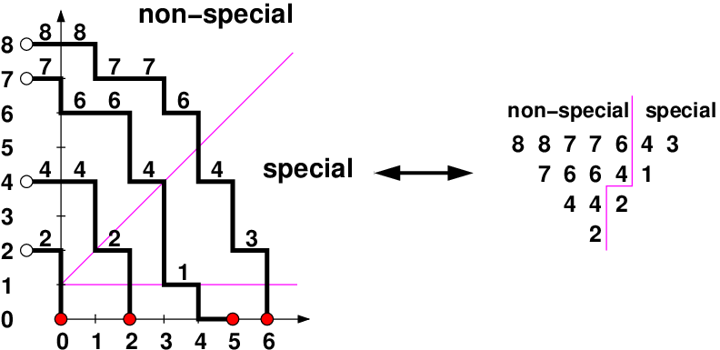
The DPPs are in bijection with configurations of non-intersecting lattice paths illustrated in Fig.2 and defined as follows. Like in Sect. 2.5, the paths take place in the positive quadrant , with the same steps but different weights and boundary conditions. The paths start along the axis at positions of the form ( recorded from right to left) and end along the axis at positions ( recorded from top to bottom). We add a final horizontal left step at the end of each path. Reading paths from left to right and top to bottom, we record the vertical positions of the -th horizontal step from the left taken on the -th path from top (steps with are not recorded). These form a DPP with rows, of order any . Conversely to each DPP with rows we may associate such a path configuration. Note that the starting points are such that , where the total number of parts in the row .
The special parts correspond to horizontal steps taken in the strict upper octant of the plane, and the remaining parts correspond to the horizontal steps in the domain , while horizontal steps along the x axis do not count (weight ).
4.2 Computation of
The computation of uses the Lindström-Gessel-Viennot [21, 14] determinant formula expressing the partition function for non-intersecting lattice paths with fixed atarting points and endpoints as a determinant where is the partition function for a single path from the -th starting point to the -th endpoint. This leads to the following:
Theorem 4.1.
[4] The partition function for DPPs of order with weight per special part and per other part reads:
| (4.1) |
where the determinant is that of the finite truncation to the first rows and columns of the infinite matrix , , with generating function:
| (4.2) |
Again, note the close similarity between the matrix and the transfer matrix for Lorentzian triangulations. Our proof of the ASM-DPP conjecture will be based on this similarity. Note also that in the notations of Appendix A.2, we have .
Let us now sketch the proof of Theorem 4.1. The sought after partition function is a sum over all configurations of non-intersecting paths () with fixed starting points , and endpoints , . According to the Lindström-Gessel-Viennot theorem, this is the sum over minors of the matrix whose entries is the partition function for a single path from to . It also has the simple expression:
Such a path is split into three pieces: (i) between the axis and the first hit on the axis (ii) between the axis and the diagonal line (iii) between the diagonal line and the vertical axis . Each piece receives a specific weight, with total contribution:
| (4.3) |
where we have first summed over (i) paths from to with horizontal steps along the axis and one final vertical step (ii) paths from to on the diagonal , for which horizontal steps must be chosen among a total of , each weighted by as these correspond to special parts (iiii) paths from to for which horizontal steps must be chosen among a total , each weighted by as they correspond to non-special parts with one extra factor for the additional final horizontal step.
Note that the matrix elements of are independent of . We may therefore consider the extension of to an infinite matrix with matrix elements given by of eqn.(4.3), for . The theorem follows by identifying the infinite matrix with , and therefore with .
5 Proof of the ASM-DPP conjecture
5.1 Proof of
The expressions (3.4) and (4.1) for respectively the partition functions and are determinants of the principal minor of size of some infinite matrix, in other words, these are the determinants of a finite truncation to the first rows and columns of infinite matrices.
There is a very simple relation (independent of ) between the generating functions of the two infinite matrices and , namely:
| (5.1) |
as a direct consequence of (3.5).
Let us translate this back into a finite matrix relation upon truncation. First, for any matrix with generating function the function is actually the generating function of the infinite matrix where is the strictly lower triangular shift matrix with elements for , and its strictly upper triangular transpose. Upon truncation to indices in , we have the obvious relation (see Lemma A.2 in Appendix A): , due to lower triangularity of and upper triangularity of . Note that both matrix truncations are unitriangular, hence have determinant so that for all . By the identity (5.1), we therefore conclude that the truncations and have the same determinant, and the version of Theorem 1.1 follows.
5.2 Refinement: proof of the MRR conjecture
The observable for ASMs may be included by slightly modifying the homogeneous limit of the IK determinant. We simply have to consider vertex weights with homogeneous limits in at points , and of the square grid, and different weights for the last column and . Defining further
gives an extra contribution to the ASM enumeration.
Adapting the method of enumeration described above, one finds that we simply have to change the definition of the last column of to include the dependence. This in turn is obtained by modifying all columns of index in the infinite matrix (we refer the reader to [4] for the technical details). The result is the following:
Theorem 5.1.
The quantity is the determinant of the truncation to the first rows and columns of the modified infinite matrix , with double generating function
The prefactor is ad-hoc and comes from a modification of the columns and higher in the infinite matrix to make it simpler. Note that the new infinite matrix has an explicit dependence on .
Likewise, keeping track of the observable in a DPP is easy. The lattice path formulation still holds and yields a LGV-like determinant as well, but for a modified matrix , identical to of (4.3) for and and with a different last column, explicitly depending on .
The latter dependence is the result of decomposing further the piece (iii) of the DPP (see Sect.4.2), when , into and and attaching weights as follows: (iii-a) the piece of the path from to its first vertex on the line at with a total of paths all with weight and (iii-b) the straight path from to with an extra weight of . This gives:
| (5.2) |
This leads to the following:
Theorem 5.2.
The quantity is the determinant of the truncation to the first rows and columns of the modified infinite matrix , with double generating function:
Like , the infinite matrix has an explicit dependence on .
The proof of the complete Mills-Robbins-Rumsey conjecture follows from the following elementary lemma, easily proved by direct computation:
Lemma 5.3.
We have the relation:
As explained above, such a relation between the two infinite matrices and guarantees that the determinant of their truncation to their first rows and columns coincide, for any , so it holds in particular for and Theorem 1.1 follows.
5.3 More refinements
In [5] a further observable was considered for ASMs and DPPs. For any ASM let be the number of entries to the right of the unique in the bottom row of . For any DPP of order , let be the number of parts equal to plus the number of rows of length . Defining the two following partition functions:
for respectively ASMs of size and DPPs of order , we have:
Theorem 5.4.
[5] We have the identity:
6 Conclusion
6.1 ASM,DPP,TSSCPP, FPL,DPL, etc.
In these notes, we have detailed the refined enumeration of ASMs and DPPs and established an identity between them.

One could think of further refinements, leading eventually to a bijection between these objects. This is however only the tip of a much larger iceberg (see Fig.3), which on the pure combinatorics side involves other objects: the so-called TSSCPPs (Totally Symmetric Self-Complementary Plane Partitions) which are yet another kind of plane partitions, with a formulation in terms of different configurations of non-intersecting lattice paths (see for instance [6] for a detailed account). There is also a statistical physics side, involving the so-called Fully Packed Loop (FPL) model on a square grid, whose configurations are in bijection with those of the 6V-DWBC model. The latter plays a central role in the so-called Razumov-Stroganov (RS) conjecture [23] proved by Cantini-Sportiello [7], relating its refined enumeration according to link patterns of connections of the loops around the grid to the asymptotic probabilities of connections of the Densely Packed Loop (DPL) model on a semi-infinite cylinder of finite perimeter. The latter is yet another integrable lattice model based on some pictorial representation of the Temperley-Lieb algebra, whose groundstate vector is a solution to the quantum Knizhnik-Zamolodchikov (qKZ) equation [9, 10]. Finally, there is an algebraic geometry side of the iceberg. For instance, the degree of the variety of upper triangular complex matrices with vanishing square corresponds to a refined enumeration of TSSCPPs, and the (equivariant cohomology) multidegree is obtained via a specialization of the solution to the qKZ equation [11].
Many of the known enumerations of the above objects involve determinants,. In a number of cases, these can be obtained through some application of the Lindström-Gessel-Viennot theorem. This applies to all the “free fermion” cases that are in bijection with non-intersecting lattice path configurations. However, both the 6V model and the DPL model are models of interacting fermions, in which even if there is some kind of lattice path formulation, the latter are no longer just non-intersecting. For instance, in the case of the 6V model, one can define paths going from the left border of the grid to the top border, by going right and up along the oriented edges as much as possible (i.e. when there is a choice, always go up). Such paths are now “osculating” in that two paths can bounce against each other at a vertex (the first going right, then up; the second going up then right; this corresponds to the vertex of the 6V model), and this configuration receives a different weight, interpreted as the exponential of some interaction energy. Yet, somehow, our formula for the refined enumeration has magically disentangled this interaction, to make it look like a free fermion model, via our determinant evaluation. This mechanism deserves to be better understood.
6.2 Integrabilities
The 6V model is the archetype of 2D integrable lattice model, related to the 1D quantum XXZ spin chain for . It is know to have an infinite family of transfer matrices provided the Boltzmann weights satisfy the following relation:
This constant is the anisotropy of the associated quantum spin chain. Alternatively, in terms of the variables of (3.2), this turns into the following “6V” variety:
| (6.1) |
as .
On the other hand, the infinite matrix , whose finitely truncated determinant gives the DWBC homogeneous 6V partition function on a grid of same size, also involves a transfer matrix of a form analogous to that of 1+1D Lorentzian triangulations, generated by:
The transfer matrices commute for different values of the parameters provided they belong to the following “Lorentzian” variety:
| (6.2) |
obtained by rephrasing (2.4) above.
Comparing (6.1) and (6.2), we see that , hence the two varieties are distinct! However, they do intersect. Solving for and with say , we find that
Conversely, any such point for lies at the intersection of two “integrable” varieties of the form (6.1) and (6.2). This intriguing fact deserves a better understanding. In particular, the 6V variety involves commutation of finite size transfer matrices, whereas the Lorentzian one concern matrices of infinite size.
Appendix A Infinite matrices and truncated determinants
Throughout these notes, we make extensive use of generating functions for infinite matrices. Let us summarize here the main definitions and properties we use.
A.1 Infinite matrices
We consider infinite matrices . The very concept of an infinite matrix is a bit delicate to work with, for instance the product of two such matrices might not be well defined. This may be repaired by introducing a formal expansion parameter , and associating to the matrix . The product of any two such matrices now makes sense in the sense of formal power series of . Moreover, even the notion of eigenvector and eigenvalue make sense in this setting, provided one can show that the latter have formal power or Laurent series expansions in .
A.2 Generating functions for infinite matrices
For an infinite matrix and a vector we define the formal generating functions
with the following properties for matrices and a vector :
where the contour integral picks the constant term in .
We consider the lower and upper triangular matrices and with generating functions
| (A.1) |
with . Let us also introduce the shift matrix and the transfer matrix generated respectively by:
| (A.2) |
In particular, we have
The case of the infinite transfer matrix for Lorentzian triangulations corresponds to the identification:
We have the following properties easily derived by contour integrals for the corresponding generating functions:
| (A.3) | |||||
| (A.4) | |||||
| (A.5) | |||||
| (A.6) | |||||
| (A.7) | |||||
| (A.8) | |||||
| (A.9) |
These hold whenever the denominators are non-vanishing.
A.3 Commuting families and addition formulas
Using the formulas above, it is easy to derive the following:
Theorem A.1.
The following family of infinite matrices commute among themselves for any fixed values of and :
We also have the following “addition” formula:
For , we obtain a family of commuting lower triangular matrices
with the “addition” formula:
Changing variables from to , with , and writing we finally get the addition formula:
| (A.10) |
from which we deduce that is an infinite matrix exponential. More precisely, let be the infinite matrix generated by
then we have , which by triangularity holds for any finite truncation as well. A similar analysis holds for , but only for the infinite matrix. Assuming that , and introducing another parameter , the relevant change of variables is:
in terms of which
This reduces to (A.10) when (corresponding to ).
A.4 Truncated determinants
For any infinite matrix , we denote by the finite truncation of to its first rows and columns, namely the matrix with entries: .
In general, the matrix product does not respect truncation. However, if are respectively lower and upper triangular infinite matrices, then . Note that this does not hold for (see the example below).
Let us now examine truncated determinants, namely the determinant of such finitely truncated matrices. By triangularity it is immediate to compute:
| (A.11) |
and by the above property we deduce from (A.6) and (A.11) that:
and more generally
whereas
by use of (A.7). The discrepancy with the result is because the matrix product now involves all the elements of the infinite and infinite rectangular matrices of the truncated product.
The main property allowing for proving truncated determinant identities from relations between generating functions is the following:
Lemma A.2.
Let be respectively lower triangular, upper triangular and arbitrary infinite matrices, and let . Then:
Assuming further that both and are unitriangular, we then deduce that for all . So we will have identity between all truncated determinants of two infinite matrices and if there is a relation for lower and upper unitriangular infinite matrices.
References
- [1] G. Andrews, Plane partitions. III. The weak Macdonald conjecture, Invent. Math. 53 (1979), No. 3, 193–225 and MacdonaldÕs conjecture and descending plane partitions, Combinatorics, representation theory and statistical methods in groups, Lecture Notes in Pure and Appl. Math., vol. 57, Dekker, New York, (1980), pp. 91–106.
- [2] J. Ambjorn and R. Loll, Non-perturbative Lorentzian quantum gravity, causality and topology change Nucl. Phys. B 536 (1998) 407–434.
- [3] M.T. Batchelor, J. de Gier and B. Nienhuis, The quantum symmetric XXZ chain at , alternating sign matrices and plane partitions, J. Phys. A 34 (2001) L265–L270. cond-mat/0101385.
- [4] R. Behrend , P. Di Francesco and P. Zinn-Justin , On the weighted enumeration of Alternating Sign Matrices and Descending Plane Partitions. J. Combin. Theory Ser. A 119 (2) (2012), 331–363. arXiv:1103.1176.
- [5] R. Behrend , P. Di Francesco and P. Zinn-Justin , The doubly refined enumeration of Alternating Sign Matrices and Descending Plane Partitions. (2012), arXiv:1202.1520.
- [6] D. Bressoud, Proofs and confirmations: The story of the alternating sign matrix conjecture, MAA Spectrum, Mathematical Association of America, Washington, DC (1999), 274 pages.
- [7] L. Cantini and A. Sportiello, Proof of the Razumov-Stroganov conjecture, Journal: J. Comb. Theory A 118 (2011) 1549–1574. arXiv:1003.3376.
- [8] P. Di Francesco, E. Guitter, and C. Kristjansen, Integrable 2D Lorentzian gravity and random walks, Nucl. Phys. B567 No. 3 (2000), 515–553. arXiv:hep-th/9907084.
- [9] P. Di Francesco and P. Zinn-Justin , Around the Razumov-Stroganov conjecture: proof of a multi-parameter sum rule. Electron. J. Combin. 12 (2005), Research Paper 6, 27 pp. arXiv:math-ph/0410061.
- [10] P. Di Francesco and P. Zinn-Justin , Quantum Knizhnik-Zamolodchikov Equation, Totally Symmetric Self-Complementary Plane Partitions and Alternating Sign Matrices. Theor. Math. Phys. 154 (3) (2008), 331–348. arXiv:math-ph/0703015.
- [11] P. Di Francesco and P. Zinn-Justin , Quantum Knizhnik-Zamolodchikov equation, generalized Razumov-Stroganov sum rules and extended Joseph polynomials, J. Phys. A: Math. Gen. 38 (2005) L815-L822. arXiv:math-ph/0508059
- [12] C. Dodgson, Condensation of determinants, Proceedings of the Royal Soc. of London 15 (1866) 150–155.
- [13] S. Fomin and A. Zelevinsky Cluster Algebras I. J. Amer. Math. Soc. 15 (2002), no. 2, 497–529 arXiv:math/0104151 [math.RT].
- [14] I. M. Gessel and X. Viennot, Binomial determinants, paths and hook formulae, Adv. Math. 58 (1985) 300–321.
- [15] A. Izergin, Partition function of the six-vertex model in a finite volume, Sov. Phys. Dokl. 32 (1987) 878–879.
- [16] A. Knutson, T. Tao, and C. Woodward, A positive proof of the Littlewood-Richardson rule using the octahedron recurrence, Electr. J. Combin. 11 (2004) RP 61. arXiv:math/0306274 [math.CO]
- [17] V. Korepin, Calculation of norms of Bethe wave functions, Comm. Math. Phys. 86 (1982) 391–418.
- [18] G. Kuperberg, Another proof of the alternating-sign matrix conjecture, Int. Math. Res. Notices No 3 (1996) 139–150. arXiv:math/9712207.
- [19] P. Lalonde, Lattice paths and the antiautomorphism of the poset of descending plane partitions, Discrete Math. 271 (1Ð3) (2003) 311–319.
- [20] C. Krattenthaler, Descending plane partitions and rhombus tilings of a hexagon with a triangular hole, European J. Combin. 27 (7) (2006) 1138–1146. arXiv:math/0310188.
- [21] B. Lindström, On the vector representations of induced matroids, Bull. London Math. Soc. 5 (1973) 85–90.
- [22] W. H. Mills, D. P. Robbins, and H. Rumsey, Alternating sign matrices and descending plane partitions, J. Combin. Theory Ser. A 34 (1983), 340–359.
- [23] A.V. Razumov and Yu.G. Stroganov, Combinatorial nature of ground state vector of O(1) loop model, Theor. Math. Phys. 138 (2004) 333–337; Teor. Mat. Fiz. 138 (2004) 395–400. arXiv:math.CO/0104216.
- [24] W. Mills, D. Robbins, H. Rumsey Jr., Proof of the Macdonald conjecture, Invent. Math. 66 (1) (1982) 73–87; D. Robbins and H. Rumsey, Determinants and alternating sign matrices, Adv. Math. 62 (1986), 169–184.
- [25] D. Zeilberger, Proof of the alternating sign matrix conjecture, Elec. J. Comb. 3 (2) (1996), R13.
Institut de Physique Théorique du Commissariat à l’Energie Atomique,
Unité de Recherche associée du CNRS,
CEA Saclay/IPhT/Bat 774, F-91191 Gif sur Yvette Cedex,
FRANCE.
E-mail: philippe.di-francesco@cea.fr