Two constructions of Markov chains on the dual of $U(n)$

This paper will examine a family of Markov processes on the state space $\{\lambda_{1}\geq\ldots\geq\lambda_{n}:\lambda_{i}\in\mathbb{Z}\}.$ These Markov processes were first introduced as the Charlier process in [12]. In [3], the authors introduce a family of Markov chains on the Gelfand–Tsetlin set $\mathbb{GT}$. This is the set of infinite sequences $\lambda^{(1)}\prec\lambda^{(2)}\prec\ldots,$ where $\lambda^{(k)}=(\lambda^{(k)}_{1}\geq\ldots\geq\lambda^{(k)}_{k})$ is a $k$–tuple of nonincreasing integers and $\lambda\prec\mu$ denotes the condition $\mu_{1}\geq\lambda_{1}\geq\mu_{2}\geq\lambda_{2}\geq\ldots\mu_{n}\geq\lambda_{n}$. By considering the map

these Markov chains define an interacting particle system on $\mathbb{Z}\times\mathbb{Z}_{+}$. Drawing lozenges around each particle yields a random tiling of the half plane. Furthermore, the condition $\lambda^{(k)}\prec\lambda^{(k+1)}$ ensures that there is a natural interpretation as a randomly growing stepped surface. This random growth belongs to the $2+1$ anisotropic KPZ class of stochastic growth models. This universality class is a variant of the KPZ universality class, which has seen many results in recent years (see [7] for a survey). By considering suitable projections, the Markov chains also reduce to TASEP, PushASEP (introduced in [4]) , and the Charlier process from [12].

The Gelfand–Tsetlin set parametrises the branching of irreducible representations of the unitary group. Additionally, the family of Markov chains can be constructed from the representation theory of the infinite–dimensional unitary group $U(\infty)$ [6]. Tools from representation theory have yielded a rich variety of two–dimensional dynamics (e.g. [9, 15]). One of the most general processes arising from representation theory are Macdonald processes [5].

In this paper, we hope to deepen the connections between probability theory and representation theory. To this end, we give two new representation–theoretic constructions for these Markov chains. The first involves the Littlewood–Richardson rule for decomposing tensor products of irreducible representations of $U(n)$. The second involves a quantum random walk on the von Neumann algebra of $U(n)$, which is then restricted to the center. These constructions have the advantage of not requiring infinite–dimensional representation theory and are therefore more generalisable to other simple Lie groups.

The structure of the paper is as follows. In section 2, we review the representation theory of $U(n)$ and introduce the Markov chains from [3]. In section 3, we provide a construction the combinatorial description of the Littlewood–Richardson coefficients. In section 4, we provide another construction, this time using a quantum random walk on the von Neumann algebra of $U(n)$. This will also give a representation theoretic explanation (i.e. using tensor products of representations instead of combinatorics) for the occurrence of the Littlewood–Richardson coefficients.

From Lemma 3.4 and (2) of [6], the measures $\mathbb{P}_{n}(\boldsymbol{\theta};F)(\mu)$ have a nice algebraic interpretation from the formula

In words, the measures $\mathbb{P}_{n}(\boldsymbol{\theta};F)$ are the coefficients in the decomposition of the function $F(\theta_{1})\cdots F(\theta_{n})$ over the normalized irreducible characters of $U(n)$. However, these measures are obtained by applying $T_{n}(\boldsymbol{\theta};F)$ to the initial condition $\boldsymbol{0}$, and it is not clear what algebraic structure remains if started from a different initial condition. Theorem 3.1 below will provide a generalization to the case when the initial condition is some nonzero $\lambda\in\mathcal{W}_{n}$. It also worth noting that for $F=F_{\alpha^{+}}$, a similar theorem has appeared in the case of the orthogonal groups, using Pieri’s formula (see [8],[13]). The theorem has also found use in [14].

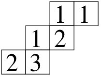
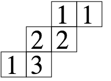
Before proceeding to the statement of Theorem 3.1, let us briefly recall the Littlewood–Richardson coefficients. For any two paritions $\lambda,\tau$ such that $\lambda_{j}\leq\tau_{j}$ for each $j$, the skew diagram of $\tau\backslash\lambda$ is the set–theoretic difference of the Young diagrams of $\lambda$ and $\tau$. A skew Tableau of shape $\tau\backslash\lambda$ and weight $\mu$ is obtained by filling in the skew diagram of $\tau\backslash\lambda$ with positive integers such that the integer $k$ appears $\mu_{k}$ times. A skew Tableau is semistandard if it the entries weakly increase along each row and strictly increase down each column. A Littlewood–Richardson tableau is a semistandard skew Tableau with the additional property that in the sequence obtained by concatenating the reversed rows, every initial part of the sequence contains any number $k$ at least as often as it contains $k+1$. See figure 1 for two examples. The Littlewood–Richardson coefficient $c_{\lambda\mu}^{\tau}$ counts the number of Littlewood–Richardson tableaux of shape $\tau\backslash\lambda$ and of weight $\mu$. In the example in figure 1, $c^{\tau}_{\lambda\mu}$ equals $2$.

In the special case $\mu=k0^{n-1}$, the Littlewood–Richardson rule is known as Pieri’s formula. In this case, the semistandard skew Tableau can only be filled with $1$’s, so the condition on the concatenated sequence is automatically satisfied. The only requirement is that the skew diagram of $\tau\backslash\lambda$ does not contain two boxes in the same column. In other words,

We also need the special case $\mu=1^{k}0^{n-k}$. The integers appearing in the semistandard skew Tableau are $\{1,2,\ldots,k\}$, so the condition on the concatenated sequence can only hold if the skew diagram of $\tau\backslash\lambda$ does not contain two boxes in the same row. In other words,

The Littlewood-Richardson coefficients are related to representation theory by the decomposition

Since the character of $V_{\lambda}$ is the Schur polynomial $s_{\lambda}$ it is equivalent to say

Note that this implies the identity $c^{\tau}_{\lambda\mu}=c^{\tau}_{\mu\lambda}$, which would not have been obvious from the combinatorial description. Also note that this allows for a natural definition of $c^{\tau}_{\mu\lambda}$ when one of $\tau,\mu,\lambda$ has negative entries. Namely, letting $\mathbf{1}=(1,1,\ldots,1)$, since $s_{\lambda+\mathbf{1}}(x_{1},\ldots,x_{n})=x_{1}\cdots x_{n}s_{\lambda}(x_{1},\ldots,x_{n})$, we can define

Also define the coefficients $c_{\lambda\sigma\mu}^{\tau}$ by

It follows immediately that

The theorem can now be stated.

Let us introduce some notation, which will follow [1] closely.

Let $G$ be a compact topological group, let $dg$ denote its Haar measure (normalized to have total weight $1$), and let $H=L^{2}(G,dg)$ be the Hilbert space of square–integrable functions. Let $\alpha$ denote the representation of $G$ on $H$ by left translation. In other words, for $f\in B(H)$ a unitary operator on $H$, the map $\alpha:G\rightarrow B(H)$ is defined by $[\alpha(g)(f)](x)=f(xg)$. The von Neumann algebra of $G$, denoted $vN(G)$, is the closure (under the strong operator topology) of the $*$–subalgebra of $B(H)$ generated by $\alpha(G)$.

Let $\kappa$ be a continuous, positive type function on $G$ which sends the identity to $1$. This defines a state $\varphi$ on $vN(G)$ by $\varphi(\alpha(g))=\kappa(g)$, and also defines a completely positive map $Q_{n}(\kappa)$ on $vN(G)$ by $[Q_{n}(\kappa)](\alpha(g))=\kappa(g)\alpha(g)$.

Since $vN(G)$ is a unital $C^{*}$–algebra, we can define the infinite tensor product $vN(G)^{\otimes\infty}$, which is also a $C^{*}$–algebra. Let $\varphi^{\otimes\infty}$ be the state on $vN(G)^{\otimes\infty}$ defined by $\varphi^{\otimes\infty}(x_{1}\otimes x_{2}\otimes\cdots)=\varphi(x_{1})\varphi(x_{2})\ldots$. The Gelfand–Naimark–Segal construction produces a von Neumann algebra $\mathcal{A}$. For nonnegative integers $k$, define $j_{k}:vN(G)\rightarrow\mathcal{A}$ by $j_{0}(\alpha(g))=Id$. and $j_{k}(\alpha(g))=\alpha(g)^{\otimes k}\otimes Id\otimes Id\otimes\cdots$. The $j_{k}$ form what is called a “non-commutative Markov process”. There is a projection map $E_{k}$ from $\mathcal{A}$ to $\mathcal{A}_{k}$, the von Neumann subalgebra generated by the images of $j_{0},\ldots,j_{k}$. For $k\leq m$, there is the Markov property $E_{k}\circ j_{m}=j_{k}\circ Q_{n}^{m-k}$. One could think of these objects with the following analogy:

References

• [1] Biane P. Quantum random walk on the dual of S​U​(n).SU(n). Probab. Th. Rel. Fields 89, 117–129 (1991).
• [2] Biane P. Miniscule weights and random walks on lattices. Quantum Probability and Related Topics Vol. VII, 51–65 (1992).
• [3] Borodin, A.; Ferrari, P.L. Anisotropic growth of random surfaces in 2+1 dimensions. J. Stat. Mech. (2009) P02009. arXiv:0804.3035v1
• [4] Borodin, A.; Ferrari, P.L. Large time asymptotics of growth models on space-like paths I: PushASEP. Elec. J. Prob, Bolume 13, Number 50 (2008), 1380–1418. arXiv:0707.2813
• [5] Borodin, A; Corwin, I. Macdonald processes arXiv:1111.4408
• [6] Borodin, A.; Kuan, J. Asymptotics of Plancherel measures for the infinite-dimensional unitary group. Adv. Math. 219 (2008), 894–931. arXiv:0712.1848v1
• [7] Corwn, I. The Kardar-Parisi-Zhang equation and universality class. arXiv:1106.1596
• [8] Defosseux, M. An interacting particle model and a Pieri-type formula for the orthogonal group. J. Theor. Probab, Feb 2012. arXiv:1012.0117v1
• [9] Defosseux, M. Interacting particle models and the Pieri-type formulas : the symplectic case with non equal weights. http://arxiv.org/abs/1104.4457
• [10] Dixmier, J. Les C *-algèbres et leurs représentations. Paris: Gauthier-Villars 1964
• [11] Fulton, W.; Harris, J. Representation theory: a first course. Graduate Texts in Mathematics, Vol. 129. Springer, New York, 1991.
• [12] König, W; O’Connell, N; Roch, S; Non–colliding random walks, tandem queues and discrete orthogonal polynomial ensembles, Elec. J. Prob, Volume 7, Number 1 (2002), 1–24.
• [13] Kuan, J. Discrete-time particle system with a wall and representations of O(infinity) . arXiv:1203.1660v1
• [14] Kuan, J. A (2+1)–dimensional Gaussian field as fluctuations of quantum random walks on quantum groups. arXiv:1601.04402v1
• [15] Warren, J; Windridge, P. Some Examples of Dynamics for Gelfand–Tsetlin Patterns. Elec. J. Prob, Volume 14, Number 59 (2009), 1745–1769. arXiv:0812.0022