Dictionary Subselection Using an Overcomplete Joint Sparsity Model

The sparse signal model is one the most successful low-dimensional signal models for modern signal processing applications [1]. In this model, any considered signal $\mathbf{y}\in\mathbb{R}^{m}$, can be represented as the sum of a few elementary functions, called the atoms, plus some noise $\mathbf{n}\in\mathbb{R}^{m}$, as follows,

where $\mathbf{D}\in\mathbb{R}^{m\times p}$, called the dictionary, is the collection of the atoms and $\mathbf{x}\in\mathbb{R}^{p}$ is a sparse vector. In this setting, $\mathbf{y}$ is often called a sparse signal in $\mathbf{D}$. The additive noise is used to consider the inaccuracy of the measurement device or the model mismatch. While choosing an overcomplete dictionary, i.e. $p>m$, gives us a flexibility to choose sparser representation, the extra redundancy can be damaging in ducking failures coefficient recovery. Therefore, the success of sparse signal models depends on how well we choose a redundant $\mathbf{D}$, which is the main focus of this paper.

There is a lot of interest in building redundant dictionaries to make more flexible models and various techniques have already been proposed to design the dictionary using some domain knowledge, see for example [2], or learning the dictionary using a given set of exemplars [3], see [4] and [5] for a more complete review on different dictionary selection techniques. The advantage of the first approach is the possibility of incorporating already known signal structures and often fast implementation of the dictionary. The second approach does not need such prior information about the signals, but they often find an unstructured dictionary with a computationally expensive implementation. We will combine these two methods in this paper, by considering a large set of potentially good atoms $\mathbf{\Phi}\in\mathbb{R}^{m\times n},\ n>p$, called a mother dictionary here, and selecting a smaller set of atoms as the final dictionary $\mathbf{D}$. Fast implementation of such dictionaries are guaranteed, if the mother dictionary has such a property. For instance, scalar products of a given signal $x$ with a family of Gabor atoms of length $m$ can be implemented with a computational complexity of $\mathcal{O}(m\log m)$. Also, as we restrict the search space to the dictionaries with mother atoms, it can be learned using much less exemplars. In other words, restricting the dictionary to a subset of mother atoms, regularises the dictionary learning problem and avoids overfitting.

As all the atoms of $\mathbf{D}$ exist in $\mathbf{\Phi}$, any sparse signal in $\mathbf{D}$, can be represented using $\mathbf{\Phi}$. The reader may ask, if we can use the large dictionary $\mathbf{\Phi}$, why we need to shrink it to find a dictionary which at best can only sparsify the signal to the same level. The answer to this question can be given by noting that, finding the sparse approximations have non-polynomial complexity, in a general setting. The success of practical sparse approximation algorithms depends on some internal structures of the dictionary, including mutual coherence [6], Restricted Isometry Property (RIP) [7] or the null-space property [8]. Dictionary size indirectly affects these properties such that larger dictionaries mostly make the sparse recovery more difficult. Roughly speaking, it is caused by the fact that putting more atoms in the dictionary, the atoms become more similar. Such similarities between different atoms, indeed make it more challenging to find which set of atoms represents the signals more accurately, i.e the problem of exact (support) recovery. The approximation in such large dictionaries would also be noise sensitive, as small noise may cause the wrong atoms to become selected. Finally, in coding, the cost of indexing which atoms being used in the representation ($\mathbf{x}$), a.k.a. the binary significance map, grows as the dictionary size increases.

Let $\mathbf{Y}=\left[\mathbf{y}_{l}\right]_{l\in[1,L]}$ be a matrix made by training samples $\mathbf{y}_{l}\in\mathbb{R}^{m}$ and $\mathbf{\Phi}=[\mathbf{\phi}_{i}]_{i\in\mathcal{I}},|\mathcal{I}|=n$ be a mother dictionary of normalised atoms $\mathbf{\phi}_{i}\in\mathbb{R}^{m}$. We assume that the generative dictionary $\mathbf{D}\in\mathbb{R}^{m\times p},\ m\leq p$ is made by a subset selection of atoms in $\mathbf{\Phi}$, i.e. $\mathbf{D}=\left[\mathbf{\phi}_{i}\right]_{i\in\mathcal{J}}$ where $\mathcal{J}\subset\mathcal{I}$ and $|\mathcal{J}|=p<n$. We assume that each $\mathbf{y}_{l}$ is approximately generated by a $k$-sparse coefficient vector $\mathbf{\gamma}_{l}$,

We want to find a dictionary that fulfils the two (apparently contradictory) objectives : few elements in the dictionary, and sparsest decomposition for each signal. In other words $\mathbf{D}$ which is both small and efficient! The problem of optimal dictionary selection can thus be defined as finding the index set $\mathcal{J}$ meeting those criteria, given $\mathbf{Y}$, $\mathbf{\Phi}$, $p$ and $k$. Let $\mathbf{X}\in\mathbb{R}^{n\times L}$ be a coefficient matrix and $f_{{\mathcal{J}}}(i):[1,p]\mapsto[1,n]$ be the mapping that assigns the corresponding atom index of $\mathbf{\Phi}$ to the $i^{th}$ component of $\gamma_{l}$. By assigning $\{{\mathbf{x}_{l}}\}_{f_{{\mathcal{J}}}(i)}\leftarrow\{{\mathbf{\gamma}_{l}}\}_{i},\ \forall i\in[1,p],\ \forall l\in[1,L]$, while the other elements of $\mathbf{X}$ are set to zero, the generative model can be reformulated as,

As $\mathbf{X}$ is $k$-sparse in each column and $p$-row-sparse, i.e. only $p$ rows of $\mathbf{X}$ have non-zero components, it lies in the intersection of the following sets,

where $\|\mathbf{\Theta}\|_{0,\infty}=\|\nu\|_{0}$, with $\{\nu\}_{i}:=\|\theta^{(i)}\|_{\infty}$ and $\theta^{(i)}$ is the $i^{th}$ row of $\Theta$. In other words, sets $\mathcal{K}$ and $\mathcal{P}$ are the sets of $n$ by $L$ matrices which respectively have $k$ non-zero elements on each column and $p$ non zero rows. The signals which can be represented using a coefficient matrix in $\mathcal{K}\cap\mathcal{P}$, the $(k,p)$-(overcomplete) joint sparse signals or, we will simply say that they follow the $(k,p)$-(overcomplete) joint sparsity model. Here, we actually combine the coefficient matrix and the dictionary parameters, i.e. the index set of optimal dictionary, in a single matrix $\mathbf{X}$, where the optimal atom indices are specified by the locations of non-zero rows of $\mathbf{X}$.

The optimal dictionary $\mathbf{D}$, which can alternatively be indicated by $\mathcal{J}$, is defined as the solution of the following problem,

$\mathbf{D}$ can actually be found using the solution of (4), by selecting the atoms of $\mathbf{\Phi}$ which have been used at least once in the representation of $\mathbf{Y}$. This formulation has some similarities with the convex formulation of Friedman et al. [19], where they combine the convex $\ell_{1}$ and $\ell_{2}$ penalties to promote an overcomplete joint sparsity model. The alternative formulation (4), used in this study, has the benefit of being directly related to the size-$p$ dictionary selection problem. Furthermore, the associated iterative algorithm, as presented in Section III offers a complexity that scales well with the dimension of the problem, that can be large in many practical problems.

Although the objective of (4) is quadratic, the optimisation of (4) subject to the non-convex constraints $\mathcal{K}$ and $\mathcal{P}$, is not easy. Most of the efficient optimisation techniques can not be used in this setting. A powerful technique, called the projected gradient, can be used when the projection onto the admissible set is available. In the space of real matrices $\mathbb{R}^{n\times L}$, the projection of a point $\mathbf{X}\in\mathbb{R}^{n\times L}$ onto a closed set $\kappa\subseteq\mathbb{R}^{n\times L}$ is defined by $\mathcal{P}_{\kappa}(\mathbf{X}):=\arg\min_{\mathbf{\Theta}\in\kappa}\|\mathbf{\Theta}-\mathbf{X}\|_{\chi}$, where $\|\cdot\|_{\chi}$ is the norm of the proposed space. We use the Hilbert - Schmidt, or Frobenius, norm here, as it is more related to the quadratic objective (3), i.e. using the same normed space, and we can analytically find the projection. In this setting, a projection onto $\ mathcal{K}$ can be found by keeping the $k$ largest coefficients of each column and letting the others be zero. The projection onto $\mathcal{P}$ can be found by keeping the $p$ rows of $\mathbf{X}$ with the largest maximum absolute values and letting the other rows be zero. Sadly, the projection onto the intersection of $\mathcal{K}$ and $\mathcal{P}$ is not analytically possible, the projected gradient algorithm can not be used in its canonical form. A property of the admissible sets $\mathcal{K}$ and $\mathcal{P}$ is that the consequent projections of a point in these sets provide a point in the intersection of them, which may indeed not necessarily be the projection onto $\mathcal{K}\cap\mathcal{P}$. The following lemma shows that alternating projection onto $\mathcal{K}$ and $\mathcal{P}$ converges in a single alternating projections.

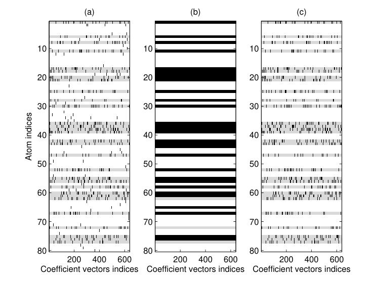
In the first experiment, a dictionary $\mathbf{\Phi}\in\mathbb{R}^{20\times 80}$ was randomly generated using a normal zero mean distribution with unit variance and normalised to have unit $\ell_{2}$-norm on each column. The target dictionary $\mathbf{D}\in\mathbb{R}^{20\times 30}$ was generated by randomly selecting $p=30$ atoms of $\mathbf{\Phi}$. A number $L=320$ of $k$-sparse coefficient vectors (with $k=4$), were generated by randomly selecting the support, with a uniform distribution of the magnitudes in $[0.2,1]$ and random signs. A set of training matrix $\mathbf{Y}$ of length $L$ were generated using the generative model and randomly generated sparse vectors. To recover the reference dictionary $\mathbf{D}$, given $\mathbf{Y}$, $p$ and $k$, we used a gradient descent based algorithm similar to Algorithm 1, with three different admissible sets, and demonstrate the superiority of the proposed technique. We first used $\mathcal{K}$ from (2) and no constraint on the row-sparsity of the coefficient matrix $\mathbf{X}$ and showed the recovered support of the sparse matrix in the left panel (a) of Figure 2. If we only assume joint sparsity model and use $\mathcal{P}$ from (3) as the admissible set, we find the coefficient matrix whose support is shown in the middle panel (b) of the same figure. Using both constraint sets, as explained in Algorithm 1, provides a coefficient matrix whose support is shown in the right panel. The correct $\mathcal{J}$ is shown in these plots using some grey lines. It is clear that the proposed projected gradient onto both sets can correctly recover $\mathcal{J}$, where the other two methods have some errors in the recovery.

This experiment can be repeated for different $\delta=\frac{p}{n}$ and $\rho=\frac{k}{m}$ by selection a range of $p$ and $k$’s, while keeping $m$ and $n$ fixed. If we repeat the simulations 100 times for each setting and calculate the average exact dictionary recovery, we can plot the phase transition for each methods. We have plotted such phase transitions in Figure 3, with $k$ sparsity constraint in (a), $p$ joint sparsity constraint in (b) and proposed constraint in (C). The black colour means high exact dictionary recovery. The area with exact recovery in (c) is larger than the same areas in (a) and (b) added together. This clearly demonstrates the relevance of the new framework.

In the next set of experiments, we will select a subset of the Curvelet [23] dictionary for the sparse representation of fingerprints. We chose a Curvelet transform for the image size $64$ by $64$. The mother dictionary $\mathbf{\Phi}\in\mathbb{R}^{4096\times 10521}$ is roughly $2.59$ times overcomplete, which we want to shrink to half size, i.e. $\mathbf{D}\in\mathbb{R}^{4096\times 5260}$. This is indeed a large scale dictionary learning problem, which is difficult to solve in a standard dictionary learning setting. With the help of the proposed method, we can handle such a big dictionary selection process, as we need fewer training samples, only need to keep a sparse matrix, i.e. sparse representation matrix, in the memory and use the fact that the mother dictionary has a fast implementation. We assume the sparsity of each image patch is $k=1052\approx 0.1N$ and $L=64$. We used two different settings here to choose the dictionary, a) $p$-joint sparsity model and b) $(k,p)$-overcomplete joint sparse model. The simulations were done in the Matlab environment, on a 12-core, 2.6 GHz linux machine, which respectively took 72 and 90 seconds to learn $\mathbf{D}_{p}$ and $\mathbf{D}_{(k,p)}$. Another fingerprint image was used to test the selected dictionaries. The original image and the $k$ sparse representation of the original image with $\mathbf{\Phi}$ are shown in the first row of Figure 4. The $k$-sparse representation with the learned $\mathbf{D}$’s are shown in the second row of this figure. The left image is the representation with learned $\mathbf{D}_{p}$, when the model was $p$-joint sparse and the right image is the same, but with $\mathbf{D}_{(k,p)}$, where the $(k,p)$-overcomplete joint sparse model was incorporated. As we can see the PSNR of the representation with the shrunk dictionary $\mathbf{D}_{(k,p)}$ is slightly better than the other. We can also see the bottom-right quarter of these images in Figure 5, in the same order. The sparse reconstructed images are actually denoised and the reconstructed image using $\mathbf{D}_{(k,p)}$ is more similar than $\mathbf{D}_{p}$ to the image reconstructed using $\mathbf{\Phi}$.

We setup a new experiment with audio signals to demonstrate the performance of the proposed dictionary selection algorithm in comparison with the fixed dictionaries and another dictionary learning method. To this end, we used some recorded audio data from BBC radio 3 (mostly classical musics), and down-sampled the signals at a sampling rate of 32 kHz, as there is very little energy above 32 kHz. We randomly selected a $\mathbf{Y}\in\mathbb{R}^{1025\times 8196}$ from more than eight hours of recorded audio. A three times overcomplete mother dictionary was generated using a two times frequency oversampled DCT plus the Delta Dirac transform, i.e. identity matrix. The reason for such a selection is to incorporate the temporal and harmonic properties of the audio. There has been a question on how useful can be to combine such dictionaries and how many DCT atoms are necessary. We thus found a subset, i.e. $p=\frac{3}{2}*1024$, of the mother atoms. If we run the proposed dictionary selection algorithm with $k=128$, for $K=1000$ iterations, and plot the frequency of appearance of the mother atoms in $\mathbf{X}$, we get the plot of Figure 6. The low-frequency DCT atoms have been used most, while high-frequency DCT atoms have not been selected in $\mathbf{D}$. Although there is no regular pattern for the selected delta Diracs, it is clear that some Dirac atoms close to the boundary of the window have been selected, i.e. close to the atom indices 2048 and 3072. If we plot the $\ell_{2}$ errors of representing a set of test data $\widehat{\mathbf{Y}}$, which is randomly selected from the same audio database, through out the IHT iterations, we get the plots of Figure 7. The $\ell_{2}$ errors corresponding to using the mother and two times overcomplete DCT dictionaries, are also shown for the reference with solid and dash-doted lines, respectively. The final SNR using the selected dictionary is slightly worse than by using the mother dictionary, but is significantly better than by using the two times overcomplete DCT. For a comparison, we also ran the sparse dictionary learning [10], with the same training data samples. The reason for selecting this dictionary learning algorithm is that it has some similarities with the proposed framework here, and it provides a relatively fast dictionary, i.e. an extra sparse matrix-vector multiplication is also necessary. To learn a dictionary for this signal size, using the canonical dictionary learning algorithms, e.g. K-SVD, MOD and MMDL [4], needs many more training samples and the computational time is very high. In the sparse dictionary learning, we used the same mother dictionary we used earlier, the objective multipliers $\lambda=\gamma=.01$ and ran the simulations for 1000 iterations. The $\ell_{2}$ errors of using the sparse learned dictionary is shown by the dotted line in Figure 7. The final SNR is not as good as when we use other dictionaries.

One aim of the proposed dictionary selection method is to provide a fast dictionary. For this reason, we measured the average calculation time of the forward and backward applications of $\mathbf{D}$ on a 2.6GHz Intel Xeon processor machine. The application of $\mathbf{D}$ and $\mathbf{D}^{T}$ as some fast operators, respectively takes, 230 and 124 ns. If Implementing the same computation as matrix-vector multiplication with the same dictionary and input data, takes 288 and 285 ns, respectively. This shows that, using a fast selected dictionary, speeds up the practical sparse approximation algorithms, as applying the dictionary and its transposed, often are the most computationally expensive parts of such algorithms.

We presented a new technique for dictionary selection for the linear sparse representation, when a collection of possibly suitable atoms and some exemplar signals are available. The dictionary selection problem is reformulated as a more general form of the joint sparse approximation problem, when the number of active locations in sparse coefficients is larger than the size of signal space. As such overcomplete joint sparsity framework has generally infinitely many solutions, the sparsity within the active set helps to regularise the problem. It was shown that the overcomplete joint sparse approximation problem is well-defined under some conditions on the null-space of the matrix generated by the given large set of atoms (mother dictionary). As the objective of the introduced program is continuously differentiable, we used a gradient mapping technique to approximately solve the problem. The introduced algorithm converges in a weak sense (convergence to a bounded non-empty set).

We presented some synthetic data simulation result to support this hypothesis that the introduced algorithm can recover the original dictionary. The phase plot of the dictionary recovery is compared with two other cases, when we use other sparsity models, namely $k$-sparse and $p$-joint sparse model. As the simulations with synthetic data were promising, we also did some simulations to select a subset of a commonly used dictionary, Curvelet and Overcomplete DCT+Dirac dictionaries, to reduce the complexity of the sparse coding algorithm. The size of dictionary learning problem is such that it cannot be handled by the vast majority of current dictionary learning algorithms. As we do not need to keep the dictionary in the memory and as the dictionary-vector multiplications can be implemented efficiently, the learning in the new framework is relatively easy. The results show that we can roughly get the same image/audio quality for a specific class of image/audio signals, when we use a smaller dictionary than the mother dictionary.

The new overcomplete joint sparsity model seems an interesting extension of the previously investigated joint sparsity model. We have left the theoretical investigation of exact recovery and other sparse signal processing applications, for the future work.

References

- [1] R. Baraniuk, V. Cevher, and M. Wakin, “Low-dimensional models for dimensionality reduction and signal recovery: A geometric perspective,” Proceedings of the IEEE, vol. 98, no. 6, pp. 959–971, 2010.
- [2] M. Yaghoobi, L. Daudet, and M. Davies, “Parametric dictionary design for sparse coding,” IEEE Transaction on Signal Processing, vol. 57, no. 12, pp. 4800–4810, 2009.
- [3] B. Olshausen and D. Field, “Sparse coding with an overcomplete basis set: a strategy employed by V1?” Vision Research, vol. 37, no. 23, pp. 3311–3325, 1997.
- [4] R. Rubinstein, A. Bruckstein, and M. Elad, “Dictionaries for sparse representation modeling,” Proceedings of the IEEE, vol. 98, no. 6, pp. 1045 – 1057, June 2010.
- [5] I. Tošić and P. Frossard, “Dictionary learning,” IEEE Signal Processing Magazine, vol. 28, no. 2, pp. 27–38, March 2011.
- [6] D. Donoho and X. Huo, “Uncertainty principles and ideal atomic decomposition,” IEEE Trans. on Information Theory, vol. 47, no. 7, pp. 2845–2862, 2001.
- [7] E. Candés and T. Tao, “Decoding by linear programming,” EEE Transaction on Information Theory, vol. 51, no. 12, pp. 4203–4215, 2005.
- [8] R. Gribonval and M. Nielsen, “Sparse representations in unions of bases,” IEEE Trans. on Information Theory, vol. 49, no. 12, pp. 3320 – 3325, 2003.
- [9] R. Neff and A. Zakhor, “Matching pursuit video coding - part I: Dictionary approximation,” IEEE Trans. on Circuits, Systems for Video Technology, vol. 12, no. 1, p. 13–26, 2002.
- [10] M. Yaghoobi and M. Davies, “Compressible dictionary learning for fast sparse approximation,” in IEEE Workshop on Statistical Signal Processing, Aug. 31- Sept. 3 2009.
- [11] R. Rubinstein, M. Zibulevsky, and M. Elad, “Double sparsity: Learning sparse dictionaries for sparse signal approximation,” IEEE Trans. on Signal Processing, vol. 58, no. 3, pp. 1553–1564, 2010.
- [12] M. Yaghoobi, T. Blumensath, and M. E. Davies, “Parsimonious dictionary learning,” in IEEE International Conference on Acoustics, Speech and Signal Processing, April 2009, pp. 2869–2872.
- [13] A. Krause and V. Cevher, “Submodular dictionary selection for sparse representation,” in International Conference on Machine Learning (ICML), 2010.
- [14] A. Das and D. Kempe, “Submodular meets spectral: Greedy algorithms for subset selection, sparse approximation and dictionary selection,” in International Conference on Machine Learning (ICML), 2011.
- [15] D. Malioutov, “A sparse signal reconstruction perspective for source localization with sensor arrays,” Master’s thesis, MIT, July 2003.
- [16] S. Cotter, B. Rao, K. Engan, and K. Kreutz Delgado, “Sparse solutions to linear inverse problems with multiple measurement vectors,” IEEE Trans. on Signal Processing, vol. 53, no. 7, pp. 2477–2488, 2005.
- [17] K. Herrity, A. Gilbert, and J. Tropp, “Sparse approximation via iterative thresholding,” in International Conference on Acoustics, Speech, and Signal Processing (ICASSP), 2006.
- [18] T. Blumensath and M. Davies, “Normalized iterative hard thresholding: Guaranteed stability and performance,” IEEE Journal of Selected Topics in Signal Processing, vol. 4, no. 2, pp. 298 – 309, April 2010.
- [19] J. Friedman, T. Hastie, and R. Tibshirani, “A note on the group lasso and a sparse group lasso,” arXiv preprint arXiv:1001.0736, 2010.
- [20] Y. Lu and M. Do, “A theory for sampling signals from a union of subspaces,” IEEE Transactions on Signal Processing, vol. 56, no. 6, pp. 2334 –2345, june 2008.
- [21] T. Blumensath and M. Davies, “Sampling theorems for signals from the union of finite-dimensional linear subspaces,” IEEE Transactions on Information Theory, vol. 55, no. 4, pp. 1872 –1882, april 2009.
- [22] T. Cover and J. Thomas, Elements of Information Theory. Wiley Interscience, 1991.
- [23] E. Candes, L. Demanet, D. Donoho, and L. Ying, “Fast discrete curvelet transforms,” Multiscale Model. Simul., vol. 5, pp. 861–899, 2006.