跳到论文正文
W Papers独立论文阅读器 arXiv:1212.2249 论文正文 计算阅读时间 · 0%
引用这篇论文根据当前论文元数据生成,正式投稿前建议核对。


License: arXiv.org perpetual non-exclusive license
arXiv:1212.2249v2 [math.CO] 02 May 2014

Combinatorial Excess Intersection

Jose Israel Rodriguez ††thanks: The author is supported by the US National Science Foundation DMS-0943745.
Abstract

We provide formulas and develop algorithms for computing the excess numbers of an ideal. The solution for monomial ideals is given by the mixed volumes of polytopes. These results enable us to design numerical algebraic geometry homotopies to compute excess numbers of any ideal.

1 Introduction

Consider a homogeneous ideal ℐ⊂ℂ⁡[x0,…,xn]\fI\subset\mathbb{C}\left[x_{0},\dots,x_{n}\right], and let f1,…,fnf_{1},\dots,f_{n} be homogenous polynomials in ℐ\fI. Since (f1,…,fn)⊂ℐ\left(f_{1},\dots,f_{n}\right)\subset\fI, we have 𝐕⁡(f1,…,fn)⊃𝐕⁡(ℐ){\bf V}\left(f_{1},\dots,f_{n}\right)\supset{\bf V}\left(\fI\right). The ​e​x​c​e​s​s​i​n​t​e​r​s​e​c​t​i​o​n\emph{excessintersection} of the variety of (f1,f2,…,fn)\left(f_{1},f_{2},\dots,f_{n}\right) with respect to the variety of ℐ\fI is defined as the quasiprojective variety 𝐕⁡(f1,…,fn)\𝐕⁡(ℐ){\bf V}\left(f_{1},\dots,f_{n}\right)\backslash{\bf V}\left(\fI\right). We define the ​e​x​c​e​s​s​n​u​m​b​e​r\emph{excessnumber} E∙​(ℐ,f1,…,fn)E_{\bullet}\left(\fI;f_{1},\dots,f_{n}\right) of an ideal ℐ\fI to be the number of solutions in 𝐕⁡(f1,…,fn)\𝐕⁡(ℐ){\bf V}\left(f_{1},\dots,f_{n}\right)\backslash{\bf V}\left(\fI\right).

Excess intersections are a well studied problem with applications in enumerative geometry, machine learning [10, 11], and algebraic statistics [9]. In addition, there is a well developed theory of Segre classes to study this problem that has been exploited in [3, 5, 12] using computational algebraic geometry as well. Recent work by Paolo Aluffi has pushed this area even further in [1]. However, the motivation for this paper came at the 2012 Institute for Mathematics and its Applications Participating Institution Summer Program for Graduate Students in Algebraic Geometry for Applications by Mike Stillman. We will focus on the numerical algebraic geometry perspective, where it is ideal to solve s​q​u​a​r​esquare systems of equations, meaning the number of unknowns equals the number of equations. So by understanding the zero-dimensional solutions of an excess intersection of an ideal, we can study the ideal itself. Our computations were performed with 𝙱𝚎𝚛𝚝𝚒𝚗𝚒{\tt Bertini}, 𝙿𝙷𝙲𝚙𝚊𝚌𝚔{\tt PHCpack}, and 𝙼𝚊𝚌𝚊𝚞𝚕𝚊𝚢𝟸{\tt Macaulay2}.

We begin our study in the case that ℐ\fI is an ideal generated by B1,B2,…,BlB_{1},B_{2},\dots,B_{l}, and f1,…,fnf_{1},\dots,f_{n} define a Bℐ−system\Bsys of equations of degree (d1,d2,…,dn)\dd.

Definition 1.

Let ℐ\fI be an ideal of ℂ⁡[x0,…,xn]\mathbb{C}\left[x_{0},\dots,x_{n}\right] generated by B1,…,BlB_{1},\dots,B_{l} whose respective degrees are p1,…,plp_{1},\dots,p_{l}. Suppose (d1,d2,…,dn)\dd is such that

min⁡(d1,d2,…,dn)≥max⁡(p1,…,pl).\min\dd\geq\max(p_{1},\dots,p_{l}).

Let ai​ja_{ij} denote a form of degree di−deg⁡Bjd_{i}-\deg B_{j}. If the forms f1,…,fnf_{1},\dots,f_{n} are given by

[f1f2⋮fn]=[a11⋯a1​la21⋯a2​l⋮⋮an​1⋯an​l]​[B1⋮Bl],\left[\begin{array}[]{l}f_{1}\\ f_{2}\\ \vdots\\ f_{n}\end{array}\right]=\left[\begin{array}[]{lll}a_{11}&\cdots&a_{1l}\\ a_{21}&\cdots&a_{2l}\\ \vdots&&\vdots\\ a_{n1}&\cdots&a_{nl}\end{array}\right]\left[\begin{array}[]{l}B_{1}\\ \vdots\\ B_{l}\end{array}\right],

then we say f1,…,fnf_{1},\dots,f_{n} are a Bℐ−system\Bsys of degree (d1,d2,…,dn)\dd.

The space of Bℐ−system\Bsys’s with degree (d1,d2,…,dn)\dd is parameterized by the coefficients of the homogeneous polynomials ai​ja_{ij}. If ℐ\fI is generated by B1,…,BlB_{1},\dots,B_{l}, then we denote the excess number of a general Bℐ−system\Bsys with degree (d1,d2,…,dn)\dd as E∙​(ℐ,d1,…,dn)\Edot.

In the first section we will be interested in determining excess numbers of Bℐ−system\Bsys’s where B1,…,BlB_{1},\dots,B_{l} are monomials.

At times it will be more convenient to work with the equivalence number

E∘​(ℐ,d1,…,dn):=d1⋯dn−E∙​(ℐ,d1,…,dn).\Ecirc:=d_{1}\cdots d_{n}-\Edot.

This definition is inspired by the notion of the equivalence of an ideal in [6] [Chapter 66]. This number is the difference between the Bezout bound and the excess number in the cases we consider. The contributions of the paper include numerical algebraic geometry algorithms to compute excess numbers and a combinatorial proof of the theorem below. This theorem can be proven easily using Fulton-MacPherson intersection theory, and in fact doing so generalizes the result to any ideal generated by a regular sequence. But in the proof we present, we will see how E∙​(ℐ,d1,…,dn)\Edot and E∘​(ℐ,d1,…,dn)\Ecirc relate to the volume of a subdivided simplex. The algorithms we present take advantage of the polyhedral structure in our problem to give bounds (lower and upper-bound) for an excess number.

Theorem 2.

Let ℐ\fI be an ideal of ℂ⁡[x0,…,xn]\mathbb{C}\left[x_{0},\dots,x_{n}\right] generated by B1,B2,…,BkB_{1},B_{2},\dots,B_{k} such that Bi=xipiB_{i}=x_{i}^{p_{i}}. If f1,…,fnf_{1},\dots,f_{n} define a Bℐ−system\Bsys of degree (d1,d2,…,dn)\dd, then

E∙(ℐ;d1,…,dn)+p1⋯pk∑δ=0n−k((−1)δ𝒟n−k−δ𝒫δ)=d1d2⋯dnE_{\bullet}\left(\fI;d_{1},\dots,d_{n}\right)+p_{1}\cdots p_{k}\sum_{\delta=0}^{n-k}\left(\left(-1\right)^{\delta}{\cal D}_{n-k-\delta}{\cal P}_{\delta}\right)=d_{1}d_{2}\cdots d_{n}

where 𝒟n−k−δ{\cal D}_{n-k-\delta} is the degree n−k−δn-k-\delta elementary symmetric function evaluated at d1,…,dnd_{1},\dots,d_{n} and PδP_{\delta} is the degree δ\delta complete homogenous symmetric function evaluated at p1,…,pkp_{1},\dots,p_{k}.

The paper is structured as follows. We consider the case when ℐ\fI is a monomial ideal, and show excess numbers equal mixed volumes of polytopes (Lemma 7). By further restricting to the case when the ideal ℐ\fI defines a complete intersection that is also a linear space (though not necessarily reduced), we do a mixed volume computation (Lemma 10) to get an explicit formula for excess numbers. In the final section, we present our algorithms that take advantage of the first sections results.

Acknowledgements

The author would like to thank Alicia Dickenstein for her many helpful comments to improve this paper as well as his advisor Bernd Sturmfels.

2 The Monomial Case

The key idea to Theorem 2 is to cast our excess intersection problem in the language of combinatorial geometry and prove Lemma 7. Since the following proofs will use Newton polytopes, Minkowski sums, and genericity, we set up additional notation here.

The ​N​e​w​t​o​n​p​o​l​y​t​o​p​e\emph{Newtonpolytope} of a form ff will be denoted as 𝒩⁡(f){\cal N}\left(f\right). The standard nn-simplex is the convex hull of the origin ϵ0\epsilon_{0}, and the standard basis of unit vectors ϵ1,…,ϵn\epsilon_{1},\dots,\epsilon_{n} in ℝn\mathbb{R}^{n}. The binary operation, Minkowski sum, will be denoted as “++”.

Now, we give examples of Bℐ−system\Bsys’s.

Example 3.

Let ℐ=(1)\fI=\left(1\right) be the trivial ideal of ℂ⁡[x0,x1]\mathbb{C}[x_{0},x_{1}] so that B1=1B_{1}=1 generates ℐ\fI. Then, a Bℐ−system\Bsys of degree d1d_{1} is given by 11 homogenous polynomials f1f_{1}

f1=a1⋅1.f_{1}=a_{1}\cdot 1.

Here, a1a_{1} is a polynomial of degree d1d_{1}. For a general choice of a1a_{1}, the excess number is d1d_{1}. When the coefficients of a1a_{1} are specially chosen the excess number can decrease. In this case, the excess number can only be less than did_{i} if the discriminant of a1a_{1} vanishes.

Whenever ℐ\fI is a principal ideal, the excess numbers are easy to determine algebraically.

Example 4.

Let ℐ=(B1)\fI=\left(B_{1}\right) be a principal ideal of the ring ℂ⁡[x0,…,xn]\mathbb{C}\left[x_{0},\dots,x_{n}\right], and let deg⁡B1=p\deg B_{1}=p. Then, a Bℐ−system\Bsys of degree (d1,d2,…,dn)\dd is given by nn homogenous polynomials f1,…,fn:f_{1},\dots,f_{n}:

f1=a1B1,f2=a2B1,…,fn=anB1.f_{1}=a_{1}B_{1},\,f_{2}=a_{2}B_{1},\dots,f_{n}=a_{n}B_{1}.

Here, aia_{i} is a polynomial of degree di−pd_{i}-p. To determine the excess number E∙​(ℐ,d1,…,dn)E_{\bullet}\left(\fI;d_{1},\dots,d_{n}\right), we saturate (f1,…,fn)\left(f_{1},\dots,f_{n}\right) by ℐ\fI. Doing so, we conclude that the excess intersection of (f1,…,fn)\left(f_{1},\dots,f_{n}\right) is defined by (a1,…,an)\left(a_{1},\dots,a_{n}\right) and consists of finitely many points. By Bezout’s theorem, it follows that E∙(ℐ;d1,…,dn)≤(d1−p)(d2−p)⋯(dn−p)E_{\bullet}\left(\fI;d_{1},\dots,d_{n}\right)\leq\left(d_{1}-p\right)\left(d_{2}-p\right)\cdots\left(d_{n}-p\right). When the aia_{i} are general polynomials of degree di−pd_{i}-p, the equality above holds.

Example 5.

Let the ideal ℐ⊂ℂ⁡[x,y,z,w]\fI\subset\mathbb{C}\left[x,y,z,w\right] be generated by the forms

B1=z2,B2=y​w,B3=y​z,B4=x​w,B5=y2,B6=x​z.B_{1}=z^{2},\>B_{2}=yw,\>B_{3}=yz,\>B_{4}=xw,\>B_{5}=y^{2},\>B_{6}=xz.

Then, a Bℐ−system\Bsys of degree (2,2,2)(2,2,2) is a system of 33 quadrics which are linear combinations of B1,…,B6B_{1},\dots,B_{6}. A general Bℐ−system\Bsys in this case has four solutions not contained in V​(ℐ)\textbf{V}(\fI). So E∙​(ℐ,2,2,2)=4E_{\bullet}(\fI;2,2,2)=4. Four is also the the mixed volume of the Newton polytopes of f1,f2,f3f_{1},f_{2},f_{3}. In Lemma , we will see that this is not a coincidence.

Example 6.

Let the ideal ℐ⊂ℂ⁡[x,y,z,w]\fI\subset\mathbb{C}\left[x,y,z,w\right] be generated by the forms

B1=z2−y​w,B2=y​z−x​w,B3=y2−x​z,B_{1}=z^{2}-yw,\>B_{2}=yz-xw,\>B_{3}=y^{2}-xz,

Then a Bℐ−system\Bsys of degree (2,2,2)(2,2,2) is a system of 33 quadrics which are linear combinations of B1,B2,B3B_{1},B_{2},B_{3}. A general Bℐ−system\Bsys in this case is equal to the ideal ℐ\fI and has no solutions outside of V​(ℐ)\textbf{V}(\fI). So E∙​(ℐ,2,2,2)=0E_{\bullet}(\fI;2,2,2)=0.

In Example 5 the excess number was a mixed volume of the Newton polytopes of fif_{i}, but in Example 6, this was not the case. Now, we explain the differences between these two situations.

Lemma 7.

Let ℐ⊂ℂ⁡[x0,…,xn]\fI\subset\mathbb{C}\left[x_{0},\dots,x_{n}\right] be an ideal defined by the monomials B1,…,BlB_{1},\dots,B_{l}. If f1,…,fnf_{1},\dots,f_{n} are a general Bℐ−system\Bsys of degree (d1,d2,…,dn)\dd, then the excess number E∙​(ℐ,d1,…,dn)\Edot equals the mixed volume of the Newton polytopes 𝒩⁡(f1),…,𝒩⁡(fn){\cal N}\left(f_{1}\right),\dots,{\cal N}\left(f_{n}\right).

Proof.

The set of Bℐ−system\Bsys’s of degree (d1,d2,…,dn)\dd is parameterized by the coefficients of ai​ja_{ij} in Definition 1. We denote the projective space associated to the coefficients of all of the polynomials ai​ja_{ij} by ℙA\mathbb{P}_{A}. The dimension of this projective space is one less than the number of coefficients of all the ai​ja_{ij}. We denote the projective space associated to the coefficients of the monomials of f1,f2,…,fnf_{1},f_{2},\dots,f_{n} as ℙC\mathbb{P}_{C}. So we have a natural map ψ\psi from ℙA\mathbb{P}_{A} to ℙC\mathbb{P}_{C} that maps the coefficients of ai​ja_{ij} to coefficients of f1,…,fnf_{1},\dots,f_{n}. Important for our situation, is that when B1,…,BnB_{1},\dots,B_{n} are monomials, the image of this map ψ\psi is onto. Let U1U_{1} denote a Zariski dense open subset of ℙA\mathbb{P}_{A} whose complement contains coefficients that give rise to Bℐ−system\Bsys’s with excess numbers less than expected. Let V2V_{2} be a Zariski dense open set of coefficients of f1,…,fnf_{1},\dots,f_{n} such that the mixed volume is less than expected. If U2U_{2} be in the inverse image of V2V_{2} under ψ\psi, then the intersection of U1U_{1} and U2U_{2} is again a Zariski dense open subset of ℙA\mathbb{P}_{A}. In particular, this means we can say a general Bℐ−system\Bsys’s for which B1,…,BlB_{1},\dots,B_{l} are monomials has E∙​(ℐ,d1,…,dn)\Edot equal to the mixed volume of 𝒩⁡(f1),…,𝒩⁡(fn){\cal N}\left(f_{1}\right),\dots,{\cal N}\left(f_{n}\right). ∎

In Example 5, ℙA\mathbb{P}_{A} equals ℙ9\mathbb{P}^{9} and ℙC\mathbb{P}_{C} equals ℙ17\mathbb{P}^{17}. By a dimension count we see that ψ\psi is not onto and explains why the mixed volume can be different from the excess number.

The key idea of this proof was the notion of a "general Bℐ−system\Bsys" so that we could use Bernstein’s theorem to count the solutions we are interested in. So to determine excess numbers of monomial ideals, we determine mixed volumes. In general, mixed volume computations are complicated, but in some cases there is hope for an explicit formula. The case we consider is when ℐ=(x1p1,…,xkpk)\fI=\left(x_{1}^{p_{1}},\dots,x_{k}^{p_{k}}\right) is generated by powers of unknowns. If f1,…,fnf_{1},\dots,f_{n} define a Bℐ−system\Bsys of degree (d1,d2,…,dn)\dd, then we determine the excess number E∙​(ℐ,d1,…,dn)E_{\bullet}\left(\fI;d_{1},\dots,d_{n}\right) by calculating the mixed volume of 𝒩⁡(f1),…,𝒩⁡(fn){\cal N}\left(f_{1}\right),\dots,{\cal N}\left(f_{n}\right). Recall that the mixed volume [13] [Chapter 8.5] can be calculated by determining the coefficient of λ1λ2⋯λn\lambda_{1}\lambda_{2}\cdots\lambda_{n} in the polynomial defining the volume of the scaled Minkowski sum

λ1​𝒩​(f1)+⋯+λn​𝒩​(fn).\lambda_{1}{\cal N}\left(f_{1}\right)+\cdots+\lambda_{n}{\cal N}\left(f_{n}\right).

If we let 𝔖\mathfrak{S} denote a simplex, then Lemma 9 shows that slicing 𝔖\mathfrak{S} by an appropriate hyperplane subdivides 𝔖\mathfrak{S} into two convex polytopes 𝔖0\mathfrak{S}_{0} and 𝔖1\mathfrak{S}_{1}. The hyperplane can be chosen so that 𝔖1=λ1​𝒩​(f1)+⋯+λn​𝒩​(fn)\mathfrak{S}_{1}=\lambda_{1}{\cal N}\left(f_{1}\right)+\cdots+\lambda_{n}{\cal N}\left(f_{n}\right). Since Vol⁡𝔖=Vol⁡𝔖0+Vol⁡𝔖1\Vol\mathfrak{S}=\Vol\mathfrak{S}_{0}+\Vol\mathfrak{S}_{1}, we compute our desired mixed volume by determining the coefficients of λ1⋯λn\lambda_{1}\cdots\lambda_{n} in Vol⁡𝔖0\Vol\mathfrak{S}_{0} and Vol⁡𝔖\Vol\mathfrak{S} (Lemma 10).

To elucidate our ideas we consider the following example.

Example 8.

Let ℐ=(x1p1,x2p2)\fI=\left(x_{1}^{p_{1}},x_{2}^{p_{2}}\right) be an ideal of the ring ℂ⁡[x0,x1,x2,x3]\mathbb{C}\left[x_{0},x_{1},x_{2},x_{3}\right] and let f1,f2,f3f_{1},f_{2},f_{3} be a Bℐ−system\Bsys of degree (d1,d2,d3)(d_{1},d_{2},d_{3}). Then the Newton polytope of fif_{i} will be the convex hull of two tetrahedra. Specifically, the Newton polytope of fif_{i} is the convex hull of the following eight points in ℝ3\mathbb{R}^{3} of which six are vertices of 𝒩⁡(fi){\cal N}\left(f_{i}\right):

(p1,0,0)(di,0,0)(p1,di−p1,0)(p1,0,di−p1)(0,p2,0)(0,di,0)(p2,di−p2,0)(p2,0,di−p2).\begin{array}[]{cccc}\left(p_{1},0,0\right)&\left(d_{i},0,0\right)&\left(p_{1},d_{i}-p_{1},0\right)&\left(p_{1},0,d_{i}-p_{1}\right)\\ \left(0,p_{2},0\right)&\left(0,d_{i},0\right)&\left(p_{2},d_{i}-p_{2},0\right)&\left(p_{2},0,d_{i}-p_{2}\right).\end{array}

To avoid confusion with points in ℙ3\mathbb{P}^{3}, we describe points in ℝ3\mathbb{R}^{3} as (u1,u2,u3)\left(u_{1},u_{2},u_{3}\right) rather than (x1,x2,x3)\left(x_{1},x_{2},x_{3}\right). We will also describe the Newton polytope 𝒩⁡(fi){\cal N}\left(f_{i}\right) by its 55 supporting hyperplanes rather than its vertices:

∙\bullet the 33 coordinate hyperplanes,

∙\bullet the hyperplane defined by u1+u2+u3−diu_{1}+u_{2}+u_{3}-d_{i}, and

∙\bullet the hyperplane defined by u1p1+u2p2−1\frac{u_{1}}{p_{1}}+\frac{u_{2}}{p_{2}}-1.
The normal vectors of the 55 hyperplanes supporting 𝒩⁡(fi){\cal N}\left(f_{i}\right) are the same for every ii. Indeed they are the standard unit vectors ϵ1,ϵ2,ϵ3\epsilon_{1},\epsilon_{2},\epsilon_{3}, the vector ϵ1+ϵ2+ϵ3\epsilon_{1}+\epsilon_{2}+\epsilon_{3}, and the vector 1p1​ϵ1+1p2​ϵ2\frac{1}{p_{1}}\epsilon_{1}+\frac{1}{p_{2}}\epsilon_{2}. By standard polytope theory [15][Proposition 7.12], it follows that the scaled Minkowski sum λ1​𝒩​(f1)+λ2​𝒩​(f2)+λ3​𝒩​(f3)\lambda_{1}{\cal N}\left(f_{1}\right)+\lambda_{2}{\cal N}\left(f_{2}\right)+\lambda_{3}{\cal N}\left(f_{3}\right), has the same 55 normal vectors as those of 𝒩⁡(fi){\cal N}\left(f_{i}\right). Indeed, the supporting hyperplanes are

∙\bullet the 33 coordinate hyperplanes,

∙\bullet the hyperplane defined by u1+u2+u3−(λ1​d1+λ2​d2+λ3​d3)u_{1}+u_{2}+u_{3}-\left(\lambda_{1}d_{1}+\lambda_{2}d_{2}+\lambda_{3}d_{3}\right), and

∙\bullet the hyperplane defined by u1p1+u2p2−(λ1+λ2)\frac{u_{1}}{p_{1}}+\frac{u_{2}}{p_{2}}-\left(\lambda_{1}+\lambda_{2}\right).
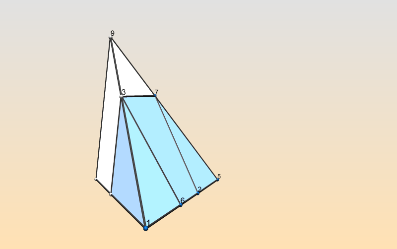
Now note that four of the five hyperplanes are defining facets of a simplex whose volume is 13!​(λ1​d1+λ2​d2+λ3​d3)3\frac{1}{3!}\left(\lambda_{1}d_{1}+\lambda_{2}d_{2}+\lambda_{3}d_{3}\right)^{3}. The fifth hyperplane subdivides the simplex as seen in Figure 11. By subtracting the volume of the white figure from the volume of the simplex, we attain the mixed volume by considering the coefficients of λ1​λ2​λ3\lambda_{1}\lambda_{2}\lambda_{3} in the difference. In this example, we would find the excess number satisfies E∙​(x1p1,x2p2,d1,d2,d3)+p1​p2​(d1+d2+d3−p1−p2)=d1​d2​d3E_{\bullet}\left(x_{1}^{p_{1}},x_{2}^{p_{2}};d_{1},d_{2},d_{3}\right)+p_{1}p_{2}\left(d_{1}+d_{2}+d_{3}-p_{1}-p_{2}\right)=d_{1}d_{2}d_{3}.

Figure 1: Refer to caption

We now precisely define the polytopes 𝔖,𝔖0,𝔖1\mathfrak{S},\mathfrak{S}_{0},\mathfrak{S}_{1}. Let D=λ1​d1+⋯+λn​dnD=\lambda_{1}d_{1}+\cdots+\lambda_{n}d_{n} and Λ=λ1+⋯+λn\Lambda=\lambda_{1}+\cdots+\lambda_{n}. Then 𝔖\mathfrak{S} is defined as the nn-simplex whose n+1n+1 vertices are the origin and D​ϵiD\epsilon_{i}. Moreover, the volume of 𝔖\mathfrak{S} equals Dn/n!D^{n}/n! which has a term d1d2⋯dnλ1λ2⋯λnd_{1}d_{2}\cdots d_{n}\lambda_{1}\lambda_{2}\cdots\lambda_{n} when expanded out. If we define the hyperplane hph_{p} by u1p1+⋯+ukpk−Λ\frac{u_{1}}{p_{1}}+\cdots+\frac{u_{k}}{p_{k}}-\Lambda, then hph_{p} slices 𝔖\mathfrak{S} into two convex polytopes 𝔖0\mathfrak{S}_{0} containing the origin, and 𝔖1\mathfrak{S}_{1}. We will prove that 𝔖1\mathfrak{S}_{1} is the scaled Minkowski sum λ1​𝒩​(f1)+⋯+λn​𝒩​(fn)\lambda_{1}{\cal N}\left(f_{1}\right)+\cdots+\lambda_{n}{\cal N}\left(f_{n}\right).

Lemma 9.

Let f1,…,fnf_{1},\dots,f_{n} be a Bℐ−system\Bsys of degree (d1,d2,…,dn)\dd. If ℐ=(x1p1,…,xkpk)\fI=\left(x_{1}^{p_{1}},\dots,x_{k}^{p_{k}}\right), then 𝔖1=λ1​𝒩​(f1)+⋯+λn​𝒩​(fn)\mathfrak{S}_{1}=\lambda_{1}{\cal N}\left(f_{1}\right)+\cdots+\lambda_{n}{\cal N}\left(f_{n}\right).

Proof.

We will show that the polytopes 𝔖1\mathfrak{S}_{1} and λ1​𝒩​(f1)+⋯+λn​𝒩​(fn)\lambda_{1}{\cal N}\left(f_{1}\right)+\cdots+\lambda_{n}{\cal N}\left(f_{n}\right) have the same n+2n+2 supporting hyperplanes so that they must be equal. Specifically, we show that the supporting hyperplanes are

∙\bullet the nn coordinate hyperplanes,

∙\bullet the hyperplane hdh_{d} defined by u1+⋯+un−Du_{1}+\cdots+u_{n}-D, and

∙\bullet the hyperplane hph_{p} defined by u1p1+⋯+ukpk−Λ\frac{u_{1}}{p_{1}}+\cdots+\frac{u_{k}}{p_{k}}-\Lambda.
The first n+1n+1 hyperplanes support the simplex 𝔖\mathfrak{S}. The last hyperplane hph_{p} slices 𝔖\mathfrak{S} into two polytopes one containing the origin and a second which is by definition the polytope 𝔖1\mathfrak{S}_{1}. Now because λi​𝒩​(fi)\lambda_{i}{\cal N}\left(f_{i}\right) has n+2n+2 supporting hyperplanes consisting of

∙\bullet the nn coordinate hyperplanes,

∙\bullet the hyperplane defined by u1+⋯+un−λi​diu_{1}+\cdots+u_{n}-\lambda_{i}d_{i}, and

∙\bullet the hyperplane defined by u1p1+⋯+ukpk−λi\frac{u_{1}}{p_{1}}+\cdots+\frac{u_{k}}{p_{k}}-\lambda_{i} .
By standard polytope theory [15][Proposition 7.12], it follows λ1​𝒩​(f1)+⋯+λn​𝒩​(fn)\lambda_{1}{\cal N}\left(f_{1}\right)+\cdots+\lambda_{n}{\cal N}\left(f_{n}\right) has the desired supporting hyperplanes. ∎

With Lemma 9, we are able to calculate the mixed volume by determining the coefficient of λ1λ2⋯λn\lambda_{1}\lambda_{2}\cdots\lambda_{n} in an integral as seen in Lemma 10.

Lemma 10.

With the previous notation, Vol⁡(𝔖0)\Vol\left(\mathfrak{S}_{0}\right) is a polynomial whose coefficient of λ1λ2⋯λn\lambda_{1}\lambda_{2}\cdots\lambda_{n} equals p1⋯pk∑δ=0n−k((−1)δ𝒟n−k−δ⋅𝒫δ)p_{1}\cdots p_{k}\sum_{\delta=0}^{n-k}\left(\left(-1\right)^{\delta}{\cal D}_{n-k-\delta}\cdot{\cal P}_{\delta}\right).

Proof.

By Lemma 9, it follows that the volume of 𝔖0\mathfrak{S}_{0} equals

Vol(𝔖0)=∫[∫⋯∫dxndxn−1⋯dxk+1]d△\Vol\left(\mathfrak{S}_{0}\right)=\int\left[\int\cdots\int d_{x_{n}}d_{x_{n-1}}\cdots d_{x_{k+1}}\right]d_{\triangle}

with the bounds of each integral inside the brackets with respect to dxid_{x_{i}} being (xi=0)→(xi=D−xi−1−⋯−x1)\left(x_{i}=0\right)\to\left(x_{i}=D-x_{i-1}-\cdots-x_{1}\right) and △\triangle denotes the simplex in kk-dimensional space with k+1k+1 vertices of ϵ0,Λ​p1⋅ϵ1,…,Λ​pk⋅ϵk\epsilon_{0},\Lambda p_{1}\cdot\epsilon_{1},\dots,\Lambda p_{k}\cdot\epsilon_{k}.

By using the calculus fact [∫⋯∫dxndxn−1⋯dxk+1]=1r!(D−xk−⋯−x1)r\left[\int\cdots\int d_{x_{n}}d_{x_{n-1}}\cdots d_{x_{k+1}}\right]=\frac{1}{r!}\left(D-x_{k}-\cdots-x_{1}\right)^{r} and the binomial theorem, we have

Vol⁡(𝔖0)=1r!​∫(D−xk−⋯−x1)r​d△=1r!​∑δ=0r((−1)δ​(rδ)​Dr−δ​∫(xk+⋯+x1)δ​d△)=p1⋯pk∑δ=0r((−1)δDn−k−δ(n−k−δ)!Λk+δ(δ+k)!𝒫δ)\begin{array}[]{lll}\Vol\left(\mathfrak{S}_{0}\right)&=&\frac{1}{r!}\int\left(D-x_{k}-\cdots-x_{1}\right)^{r}d_{\triangle}\\ &=&\frac{1}{r!}\sum_{\delta=0}^{r}\left(\left(-1\right)^{\delta}\binom{r}{\delta}D^{r-\delta}\int\left(x_{k}+\cdots+x_{1}\right)^{\delta}d_{\triangle}\right)\\ &=&p_{1}\cdots p_{k}\sum_{\delta=0}^{r}\left(\left(-1\right)^{\delta}\frac{D^{n-k-\delta}}{\left(n-k-\delta\right)!}\frac{\Lambda^{k+\delta}}{\left(\delta+k\right)!}{\cal P}_{\delta}\right)\end{array}

with r=n−kr=n-k. It is known how to integrate a linear form raised to some power over the simplex. So to get the last equality, we use [2] [Remark 99], that says ∫(xk+⋯+x1)δd△=Λk+δp1⋯pkδ!(δ+k)!𝒫δ\int\left(x_{k}+\cdots+x_{1}\right)^{\delta}d_{\triangle}=\Lambda^{k+\delta}p_{1}\cdots p_{k}\frac{\delta!}{\left(\delta+k\right)!}{\cal P}_{\delta}.

Now, note that Lm​(λ1,…,λn):=m!​(the monomials in λ1,…,λn of degree ​m)L_{m}\left(\lambda_{1},\dots,\lambda_{n}\right):=m!\left(\text{the monomials in $\lambda_{1},\dots,\lambda_{n}$\,of degree }m\right) is congruent to Λm\Lambda^{m} modulo λ12,…,λn2\lambda_{1}^{2},\dots,\lambda_{n}^{2}. Similarly, also note that DmD^{m} is congruent to Lm​(λ1​d1,…,λn​dn)L_{m}\left(\lambda_{1}d_{1},\dots,\lambda_{n}d_{n}\right) modulo λ12,…,λn2\lambda_{1}^{2},\dots,\lambda_{n}^{2}. So we have

Vol⁡(𝔖0)≡p1⋯pk∑δ=0n−k((−1)δLn−k−δ(λ1d1,…,λndn)⋅Lk+δ(λ1,…,λn)𝒫δ)≡λ1⋯λn⋅p1⋯pk∑δ=0n−k((−1)δ𝒟n−k−δ𝒫δ).\begin{array}[]{lll}\Vol\left(\mathfrak{S}_{0}\right)&\equiv&p_{1}\cdots p_{k}\sum_{\delta=0}^{n-k}\left(\left(-1\right)^{\delta}L_{n-k-\delta}\left(\lambda_{1}d_{1},\dots,\lambda_{n}d_{n}\right)\cdot L_{k+\delta}\left(\lambda_{1},\dots,\lambda_{n}\right){\cal P}_{\delta}\right)\\ &\equiv&\lambda_{1}\cdots\lambda_{n}\cdot p_{1}\cdots p_{k}\sum_{\delta=0}^{n-k}\left(\left(-1\right)^{\delta}{\cal D}_{n-k-\delta}{\cal P}_{\delta}\right).\end{array}

The last congruence is shown by an easy combinatorial argument. ∎

Remark 11.

We remark that the number E∙​(ℐ,d1,…,dn)E_{\bullet}\left(\fI;d_{1},\dots,d_{n}\right) depends only on the Newton polytopes 𝒩⁡(f1),…,𝒩⁡(fn){\cal N}\left(f_{1}\right),\dots,{\cal N}\left(f_{n}\right). For example, consider the ideals ℐ1=(x3,y3)\fI_{1}=\left(x^{3},y^{3}\right), ℐ2=(x3,y3,x2​y,xy2)\fI_{2}=\left(x^{3},y^{3},x^{2}y,xy^{2}\right), ℐ3=(x3,y3,x2​y2)\fI_{3}=\left(x^{3},y^{3},x^{2}y^{2}\right) in the ring ℂ⁡[w,x,y,z]\mathbb{C}\left[w,x,y,z\right]. All three of these ideals have the same excess numbers when every did_{i} is greater than 44 because the Newton polytopes of the defining polynomials of a Bℐ−system\Bsys are the same for i=1,2,3i=1,2,3. In particular, E∙​(ℐi,5,5,5)=44E_{\bullet}\left(\fI_{i};5,5,5\right)=44 for i=1,2,3i=1,2,3. But if we consider the ideal 𝒥=(x3,y3)+(x​y){\cal J}=\left(x^{3},y^{3}\right)+\left(xy\right), we find the Newton polytopes of a B𝒥−system\BsysJ are different from those Newton polytopes of a Bℐ−system\Bsys. In particular, one can compute the excess number E∙​(𝒥,5,5,5)E_{\bullet}\left({\cal J};5,5,5\right) to be 6565.

3 Numerical Algebraic Geometry Algorithms

We have given a combinatorial description of excess numbers of monomial ideals in the first part of the paper and used this idea to give an explicit formula in Theorem 2. In the last part of this paper, we give algorithms that use homotopy continuation, an idea from numerical algebraic geometry, to compute excess numbers of any ideal ℐ⊂ℂ⁡[x0,…,xn]\fI\subset\mathbb{C}\left[x_{0},\dots,x_{n}\right]. As mentioned in the introduction there are other ways to compute excess numbers with Segre classes. In addition, one can use off-the-shelf computer algebra software like Macaulay2 to compute excess numbers by saturating the ideal of a Bℐ−system\Bsys by ℐ\fI. Also, the examples we present here can also be worked out by hand using Fulton-MacPherson intersection theory.

Our algorithms will construct two homotopies, called 𝐡upp\hup and 𝐡ite\hit, that take the isolated solutions of a Bℐ′−system\BsysPrime f1′,…,fn′f_{1}^{\prime},\dots,f_{n}^{\prime} as start points and tracks them to solutions of f1,…,fnf_{1},\dots,f_{n} giving bounds on E∙​(ℐ,d1,…,dn)E_{\bullet}\left(\fI;d_{1},\dots,d_{n}\right). In the first algorithm, the monomial ideal ℐ′\fI^{\prime} is constructed so that E∙​(ℐ′,d1,…,dn)≥E∙​(ℐ,d1,…,dn)E_{\bullet}\left(\fI^{\prime};d_{1},\dots,d_{n}\right)\geq E_{\bullet}\left(\fI;d_{1},\dots,d_{n}\right). By doing a numerical membership test [13] [Chapter 1515], we will determine E∙​(ℐ,d1,…,dn)E_{\bullet}\left(\fI;d_{1},\dots,d_{n}\right) and isolated solutions of 𝐕⁡(f1,…,fn)\𝐕⁡(ℐ){\bf V}\left(f_{1},\dots,f_{n}\right)\backslash{\bf V}\left(\fI\right) explicitly. In the second algorithm, the monomial ideal ℐ′\fI^{\prime} is constructed to give lower bounds of E∙​(ℐ,d1,…,dn)E_{\bullet}\left(\fI;d_{1},\dots,d_{n}\right) instead. But by iterating the second algorithm, we have a probabilistic way to make this bound sharp and compute all isolated solutions of 𝐕⁡(f1,…,fn)\𝐕⁡(ℐ){\bf V}\left(f_{1},\dots,f_{n}\right)\backslash{\bf V}\left(\fI\right) explicitly. The 𝐡upp\hup-homotopy gets its name because it produces an u​p​pupper bound of E∙​(ℐ,d1,…,dn)E_{\bullet}\left(\fI;d_{1},\dots,d_{n}\right) prior to a membership test. The 𝐡ite\hit-homotopy gets its name because several i​t​eiterations can produce sharp lower bounds of E∙​(ℐ,d1,…,dn)E_{\bullet}\left(\fI;d_{1},\dots,d_{n}\right) after a membership test.

3.1 Algorithm one and the 𝐡upp\hup-homotopy

We now give a definition of the 𝐡upp\hup-homotopy and prove that it does indeed provide an upper bound of E∙​(ℐ,d1,…,dn)E_{\bullet}\left(\fI;d_{1},\dots,d_{n}\right) prior to a membership test.

Definition 12.

Let B1,…​Bl∈ℂ⁡[x0,…,xn]B_{1},\dots B_{l}\in\mathbb{C}\left[x_{0},\dots,x_{n}\right] be forms such that Bj=∑kAj,kB_{j}=\sum_{k}A_{j,k} with Aj,kA_{j,k} being a monomial multiplied by a scalar. To ease notation, let Aj→=[Aj,1,…,Aj,kj]\overrightarrow{A_{j}}=\left[A_{j,1},\dots,A_{j,k_{j}}\right] be a row vector whose entries sum to BjB_{j}, αi,j→\overrightarrow{\alpha_{i,j}} be a row vector of kjk_{j} different general forms, and βi,j→\overrightarrow{\beta_{i,j}} be a row vector of a general form that is repeated kjk_{j} times. Define the 𝐡upp\hup-homotopy as 𝐡upp⁡(t,d1,…,dn):=\hup\left(t;d_{1},\dots,d_{n}\right):=

(t​[α1,1→α1,2→⋯α1,l→⋮⋮αn,1→αn,2→⋯αn,l→]+(1−t)​[β1,1→β1,2→⋯β1,l→⋮⋮βn,1→βn,2→⋯βn,l→])​[A1→​TA2→​T⋮Al→​T],\left(t\left[\begin{array}[]{cccc}\overrightarrow{\alpha_{1,1}}&\overrightarrow{\alpha_{1,2}}&\cdots&\overrightarrow{\alpha_{1,l}}\\ \vdots&&&\vdots\\ \overrightarrow{\alpha_{n,1}}&\overrightarrow{\alpha_{n,2}}&\cdots&\overrightarrow{\alpha_{n,l}}\end{array}\right]+\left(1-t\right)\left[\begin{array}[]{cccc}\overrightarrow{\beta_{1,1}}&\overrightarrow{\beta_{1,2}}&\cdots&\overrightarrow{\beta_{1,l}}\\ \vdots&&&\vdots\\ \overrightarrow{\beta_{n,1}}&\overrightarrow{\beta_{n,2}}&\cdots&\overrightarrow{\beta_{n,l}}\end{array}\right]\right)\left[\begin{array}[]{c}\overrightarrow{A_{1}}\mbox{}^{T}\\ \overrightarrow{A_{2}}\mbox{}^{T}\\ \vdots\\ \overrightarrow{A_{l}}\mbox{}^{T}\end{array}\right],

with the degrees of the general forms of αi,j→\overrightarrow{\alpha_{i,j}} and βi,j→\overrightarrow{\beta_{i,j}} chosen so that 𝐡upp⁡(t,d1,…,dn)\hup\left(t,d_{1},\dots,d_{n}\right) is a system of nn forms of degrees d1,…,dnd_{1},\dots,d_{n}. We denote the start points of 𝐡upp\hup(t,d1,…,dn)\left(t;d_{1},\dots,d_{n}\right) as S𝐡uppS_{\hup} and take them to be the isolated solutions of 𝐡upp⁡(1,d1,…,dn)\hup\left(1;d_{1},\dots,d_{n}\right). Denote the end points of 𝐡upp\hup(t,d1,…,dn)\left(t;d_{1},\dots,d_{n}\right) as T𝐡uppT_{\hup}.

With this definition, we have when t=1t=1 that 𝐡upp⁡(t,d1,…,dn)\hup\left(t;d_{1},\dots,d_{n}\right) is a general Bℐ′−system\BsysPrime f1′,…,fn′f_{1}^{\prime},\dots,f_{n}^{\prime} of degrees (d1,d2,…,dn)\dd. On the other hand, when t=0t=0 we have 𝐡upp⁡(t,d1,…,dn)\hup\left(t;d_{1},\dots,d_{n}\right) is a Bℐ−system\Bsys of degree (d1,d2,…,dn)\dd. By the fundamental theorem of parameter continuation of isolated roots [13] [Theorem 7.1.67.1.6] it follows that T𝐡uppT_{\hup} contains all isolated solutions of f1,…,fnf_{1},\dots,f_{n}. In particular, this proves Theorem 13 because #​S𝐡upp≥#​T𝐡upp\#S_{\hup}\geq\#T_{\hup}.

Theorem 13.

Let ℐ⊂ℂ⁡[x0,…,xn]\fI\subset\mathbb{C}\left[x_{0},\dots,x_{n}\right] be generated by the forms B1,…​BlB_{1},\dots B_{l} such that Bj=∑kAj,kB_{j}=\sum_{k}A_{j,k} with Aj,kA_{j,k} being a monomial multiplied by a scalar. If we let ℐ′\fI^{\prime} be generated by Aj,kA_{j,k}, then

E∙​(ℐ′,d1,…,dn)≥E∙​(ℐ,d1,…,dn).E_{\bullet}\left(\fI^{\prime};d_{1},\dots,d_{n}\right)\geq E_{\bullet}\left(\fI;d_{1},\dots,d_{n}\right).

Moreover, the parameter homotopy 𝐡upp⁡(t,d1,…,dn)\hup\left(t;d_{1},\dots,d_{n}\right) has endpoints T𝐡uppT_{{\bf\hup}} containing all isolated solutions of f1′,…,fn′f_{1}^{\prime},\dots,f_{n}^{\prime}.

Now that we have the theorem, we present our algorithm.

𝐈𝐧𝐩𝐮𝐭{\bf Input}: Natural numbers d1,…,dnd_{1},\dots,d_{n} and generators B1,…,BlB_{1},\dots,B_{l} of an ideal ℐ\fI in ℂ⁡[x0,…,xn]\mathbb{C}\left[x_{0},\dots,x_{n}\right] such that Bj=∑kAj,kB_{j}=\sum_{k}A_{j,k}. 𝐎𝐮𝐭𝐩𝐮𝐭:{\bf Output:} The excess number E∙​(ℐ,d1,…,dn)E_{\bullet}\left(\fI;d_{1},\dots,d_{n}\right). ​S​t​e​p​1:\emph{Step1}: Construct the the 𝐡upp\hup-homotopy 𝐡upp⁡(t,d1,…,dn){\bf\hup}\left(t;d_{1},\dots,d_{n}\right). ​S​t​e​p​2:\emph{Step2:} Solve the start system 𝐡upp⁡(1,d1,…,dn):=[f1′,…,fn′]T\hup\left(1;d_{1},\dots,d_{n}\right):=\left[f_{1}^{\prime},\dots,f_{n}^{\prime}\right]^{T} and compute S𝐡uppS_{\hup}. ​S​t​e​p​3:\emph{Step3:} Use the 𝐡upp\hup-homotopy to determine T𝐡uppT_{\hup} and an upper bound of E∙​(ℐ,d1,…,dn)E_{\bullet}\left(\fI;d_{1},\dots,d_{n}\right). ​S​t​e​p​4:\emph{Step4:} Use a numerical membership test to determine E∙​(ℐ,d1,…,dn)E_{\bullet}\left(\fI;d_{1},\dots,d_{n}\right) and the isolated solutions of 𝐡upp⁡(0,d1,…,dn):=f1,…,fn\hup\left(0;d_{1},\dots,d_{n}\right):=f_{1},\dots,f_{n}.

For this algorithm, we assume in Step 22 that the excess intersection of a monomial ideal can be determined. We now give an example where ℐ\fI defines the twisted cubic.

Example 14.

Let the ideal ℐ⊂ℂ⁡[x,y,z,w]\fI\subset\mathbb{C}\left[x,y,z,w\right] be generated by the forms

B1=z2−y​w,B2=y​z−x​w,B3=y2−x​z,B_{1}=z^{2}-yw,\>B_{2}=yz-xw,\>B_{3}=y^{2}-xz,

and suppose we want to calculate E∙​(ℐ,3,3,3)E_{\bullet}\left(\fI;3,3,3\right). To run the first algorithm, we input d1=d2=d3=3d_{1}=d_{2}=d_{3}=3 and B1,B2,B3B_{1},B_{2},B_{3}. In Step 11, we determine 𝐡upp⁡(t,d1,…,dn)=\hup\left(t;d_{1},\dots,d_{n}\right)=

(t​[a11a12⋯a16a21a22⋯a26a31a32⋯a36]+(1−t)​[b11b11b12b12b13b13b21b21b22b22b23b23b31b31b32b32b33b33])​[z2−y​wy​z−x​wy2−x​z].\left(t\left[\begin{array}[]{cccc}a{}_{11}&a{}_{12}&\cdots&a{}_{16}\\ a{}_{21}&a{}_{22}&\cdots&a{}_{26}\\ a{}_{31}&a{}_{32}&\cdots&a{}_{36}\end{array}\right]+\left(1-t\right)\left[\begin{array}[]{cccccc}b_{11}&b_{11}&b_{12}&b_{12}&b_{13}&b_{13}\\ b_{21}&b_{21}&b_{22}&b_{22}&b_{23}&b_{23}\\ b_{31}&b_{31}&b_{32}&b_{32}&b_{33}&b_{33}\end{array}\right]\right)\left[\begin{array}[]{c}z^{2}\\ -yw\\ yz\\ -xw\\ y^{2}\\ -xz\end{array}\right].

The forms ai​ja{}_{ij} and bi​jb_{ij} are general linear forms of ℂ⁡[x,y,z,w]\mathbb{C}\left[x,y,z,w\right]. Once we have solved the system 𝐡upp⁡(1,3,3,3)\hup\left(1;3,3,3\right) in Step 22, we path track in Step 33 to calculate T𝐡uppT_{\hup} giving an upper bound #​T𝐡upp\#T_{\hup} of E∙​(ℐ,3,3,3)E_{\bullet}\left(\fI;3,3,3\right). In Step 44, we use a numerical membership test [13] to conclude E∙​(ℐ,3,3,3)=10E_{\bullet}\left(\fI;3,3,3\right)=10. Indeed, if

[b11b12⋮b33]=[1/214/51/31/57/8131/3379/71/841/65−1−547/88/931/151/6−8−1/421/3−1−1−27/91/4]T​[xyzw],\left[\begin{array}[]{c}b_{11}\\ b_{12}\\ \vdots\\ b_{33}\end{array}\right]=\left[\begin{array}[]{cccccccc}1/2&1&4/5&1/3&1/5&7/8&13&1/3\\ 3&7&9/7&1/8&4&1/6&5&-1\\ -5&4&7/8&8/9&3&1/15&1/6&-8\\ -1/4&2&1/3&-1&-1&-2&7/9&1/4\end{array}\right]^{T}\left[\begin{array}[]{c}x\\ y\\ z\\ w\end{array}\right],

then we find the ten excess points are s1,s2,s3,s4,s5,s6,s7,s8=s¯5,s9=s¯6,s10=s¯7s_{1},s_{2},s_{3},s_{4},s_{5},s_{6},s_{7},s_{8}=\bar{s}_{5},s_{9}=\bar{s}_{6},s_{10}=\bar{s}_{7}:

s1s2s3s4x−6.1999−0.2081−1.0024−0.1530y5.97660.59793.12080.3771z−2.3702−2.1386−5.1077−0.6183w1111,\begin{array}[]{ccccc}&s_{1}&s_{2}&s_{3}&s_{4}\\ x&-6.1999&-0.2081&-1.0024&-0.1530\\ y&5.9766&0.5979&3.1208&0.3771\\ z&-2.3702&-2.1386&-5.1077&-0.6183\\ w&1&1&1&1\end{array},
s5s6s7x−.6493+1.4057​i0.4713−0.0461​i2.9076+0.0384​iy.4134−1.4061​i0.2603−0.5271​i−1.0341+1.7553​iz−1.1267+0.3173​i−0.9278+0.1923​i−0.7082−1.2392​iw111.\begin{array}[]{cccc}&s_{5}&s_{6}&s_{7}\\ x&-.6493+1.4057i&0.4713-0.0461i&2.9076+0.0384i\\ y&.4134-1.4061i&0.2603-0.5271i&-1.0341+1.7553i\\ z&-1.1267+0.3173i&-0.9278+0.1923i&-0.7082-1.2392i\\ w&1&1&1\end{array}.

3.2 Algorithm two and the 𝐡ite\hit-homotopy

The second algorithm we present is probabilistic. The algorithm uses the 𝐡ite\hit-homotopy to compute a lower bound of excess numbers. By iterating this algorithm, the lower bounds can become sharp.

Definition 15.

Let B1,…​Bl∈ℂ⁡[x0,…,xn]B_{1},\dots B_{l}\in\mathbb{C}\left[x_{0},\dots,x_{n}\right] be forms that generate ℐ\fI and A1,…,AlA_{1},\dots,A_{l} be monomials that generate ℐ′\fI^{\prime} such that deg⁡Bj=deg⁡Aj\deg B_{j}=\deg A_{j}. The 𝐡ite\hit-homotopy is defined as 𝐡ite⁡(t,d1,…,dn):=\hit\left(t;d_{1},\dots,d_{n}\right):=

[a11a12⋯a1​l⋮an​1an​2⋯an​l]​(t​[A1⋮Al]+γ⁡(1−t)​[B1⋮Bl]),\left[\begin{array}[]{cccc}a_{11}&a_{12}&\cdots&a_{1l}\\ \vdots\\ a_{n1}&a_{n2}&\cdots&a_{nl}\end{array}\right]\left(t\left[\begin{array}[]{c}A_{1}\\ \vdots\\ A_{l}\end{array}\right]+\gamma\left(1-t\right)\left[\begin{array}[]{c}B_{1}\\ \vdots\\ B_{l}\end{array}\right]\right),

with the degrees of the general forms ai​ja_{ij} equal to deg⁡fi−deg⁡Aj\deg f_{i}-\deg A_{j}. We denote the start points of 𝐡ite\hit as SiteS_{\itt} and take them to be the isolated solutions of 𝐡ite⁡(1,d1,…,dn)\hit\left(1;d_{1},\dots,d_{n}\right) and denote the end points of 𝐡ite⁡(t,d1,…,dn)\hit\left(t;d_{1},\dots,d_{n}\right) as TiteT_{\itt}.

With this definition, we have when tt equals 11 that 𝐡ite⁡(t,d1,…,dn)\hit\left(t;d_{1},\dots,d_{n}\right) is a Bℐ′−system\BsysPrime f1′,…,fn′f_{1}^{\prime},\dots,f_{n}^{\prime} of degrees (d1,d2,…,dn)\dd. On the other hand, when t=0t=0 we have 𝐡ite⁡(t,d1,…,dn)\hit\left(t;d_{1},\dots,d_{n}\right) is a system of nn ℐ\fI-general forms of degrees d1,…,dnd_{1},\dots,d_{n}. While the 𝐡ite\hit-homotopy is easy to set up, the fundamental theorem of parameter continuation of isolated roots [13] [Theorem 7.1.67.1.6] cannot be applied. So T𝐡iteT_{\hit} does not necessarily contain all isolated solutions of f1,…,fnf_{1},\dots,f_{n}. However, after doing a membership test, we can determine some points in T𝐡iteT_{\hit} are isolated solutions of f1,…,fnf_{1},\dots,f_{n}. So what we have is a lower bound on E∙​(ℐ,d1,…,dn)E_{\bullet}\left(\fI;d_{1},\dots,d_{n}\right). But, by iterating this homotopy, we can find more isolated solutions and give a better lower bound.

𝐈𝐧𝐩𝐮𝐭{\bf Input}: Natural numbers d1,…,dnd_{1},\dots,d_{n}, generators B1,…,BlB_{1},\dots,B_{l} of an ideal ℐ⊂ℂ⁡[x0,…,xn]\fI\subset\mathbb{C}\left[x_{0},\dots,x_{n}\right], monomials A1,A2,…,AlA_{1},A_{2},\dots,A_{l} such that deg⁡Aj=deg⁡Bj\deg A_{j}=\deg B_{j}, and a (possibly empty) set WW of isolated solutions of f1,…,fnf_{1},\dots,f_{n}. 𝐎𝐮𝐭𝐩𝐮𝐭:{\bf Output:} A set WiteW_{\itt} containing WW of isolated solutions of f1,…,fnf_{1},\dots,f_{n}, and #​Wite\#W_{\itt} a lower bound for the excess number E∙​(ℐ,d1,…,dn)E_{\bullet}\left(\fI;d_{1},\dots,d_{n}\right). ​S​t​e​p​1:\emph{Step1}: Construct the 𝐡ite\hit-homotopy 𝐡ite⁡(t,d1,…,dn)\hit\left(t;d_{1},\dots,d_{n}\right) and track start solutions SiteS_{\itt} to target solutions TiteT_{\itt}. ​S​t​e​p​2:\emph{Step2:} Use a membership test to determine which solutions of TiteT_{\itt} are isolated and set WiteW_{\itt} to be the union of WW and isolated solutions of TiteT_{\itt}. ​S​t​e​p​3:\emph{Step3:} Output WiteW_{\itt} and #​Wite\#W_{\itt} OR repeat steps 1−31-3 by making a different choice of γ\gamma in the 𝐡ite\hit-homotopy.

By taking different choices of γ\gamma in the 𝐡ite\hit-homotopy we were able to produce the following example.

Example 16.

If we take A1=z2,A2=y​z,A3=y2A_{1}=z^{2},A_{2}=yz,A_{3}=y^{2} , then we have the excess number E∙​(ℐ′,3,3,3)=7E_{\bullet}\left(\fI^{\prime};3,3,3\right)=7. Next, we construct the 𝐡ite\hit-homotopy as 𝐡ite⁡(t,d1,…,dn)=\hit\left(t;d_{1},\dots,d_{n}\right)=

[b11b12b13b21b22b23b33b32b33]​(t​[z2y​zy2]+γ⁡(1−t)​[z2−y​wy​z−x​wy2−x​z])\left[\begin{array}[]{ccc}b_{11}&b_{12}&b_{13}\\ b_{21}&b_{22}&b_{23}\\ b_{33}&b_{32}&b_{33}\end{array}\right]\left(t\left[\begin{array}[]{c}z^{2}\\ yz\\ y^{2}\end{array}\right]+\gamma\left(1-t\right)\left[\begin{array}[]{c}z^{2}-yw\\ yz-xw\\ y^{2}-xz\end{array}\right]\right)

with ai​ja_{ij} the same as in Example 14. We find the 77 isolated solutions of 𝐡ite⁡(1,d1,d2,d3)\hit\left(1;d_{1},d_{2},d_{3}\right) are s1′,s2′,s3′,s4′,s¯2′,s¯3′,s¯4′s_{1}^{\prime},s_{2}^{\prime},s_{3}^{\prime},s_{4}^{\prime},\bar{s}_{2}^{\prime},\bar{s}_{3}^{\prime},\bar{s}_{4}^{\prime}:

s1′s2′s3′s4′x−8.4814−.0354+.7868​i.8876+.0702​i−.3053+.4774​iy8.2976−.1201+−.7446​i.3006−.5880​i.3779−.7007​iz−2.9043−.9638+.1650​i−1.2929+.2635​i−1.8276+.6092​iw1111.\begin{array}[]{ccccc}&s^{\prime}_{1}&s^{\prime}_{2}&s^{\prime}_{3}&s^{\prime}_{4}\\ x&-8.4814&-.0354+.7868i&.8876+.0702i&-.3053+.4774i\\ y&8.2976&-.1201+-.7446i&.3006-.5880i&.3779-.7007i\\ z&-2.9043&-.9638+.1650i&-1.2929+.2635i&-1.8276+.6092i\\ w&1&1&1&1\end{array}.

By taking γ\gamma to be different complex numbers and keeping bi​jb_{ij} fixed, with 44 iterations, we were able to find that E∙​(ℐ,d1,…,dn)E_{\bullet}\left(\fI;d_{1},\dots,d_{n}\right) has a lower bound of 1010. By the previous subsection, we know that this lower bound is actually sharp.

We comment that with some choices of A1,A2,A3A_{1},A_{2},A_{3} defining ℐ\fI, it can happen that E∙​(ℐ′,3,3,3)E_{\bullet}\left(\fI^{\prime};3,3,3\right) is greater than, equal to, or less than E∙​(ℐ,3,3,3)E_{\bullet}\left(\fI;3,3,3\right). So one may be tracking too many paths, too few paths, or perhaps luckily the right number. Open questions remain about for which choice of monomials A1,…,AlA_{1},\dots,A_{l} yield the best computational results. In addition, how should we choose γ\gamma to find new solutions as we iterate; and how can we verify that our lower bound has become sharp are also interesting questions. These questions will remain for future work, and their answers may depend heavily on the context of the problem.

Remark 17.

We remark that the 𝐡ite\hit-homotopy need not have had the AjA_{j} be monomials. Any choice of a form AjA_{j} whose degree equals BjB_{j} could have been used. However, in this section, we have made the assumption that excess intersections of monomial ideals can be computed effectively, as we saw combinatorics can be used to understand excess numbers of monomial ideals.

To conclude, we have shown that determining excess numbers of monomial ideals can be reduced to computing a mixed volume in some cases. With this idea, we are able to provide an explicit formula for excess numbers of ideals with general generators. We presented two algorithms using numerical algebraic geometry to determine excess numbers of any ideal. We also demonstrated that these algorithms have successfully lead to the calculation of excess numbers of an ideal defining the twisted cubic. We believe that the the 𝐡upp\hup-homotopy can compute excess numbers of many other ideals defined by sparse forms in many unknowns.

References

  • [1] Paolo Aluffi. Segre classes as integrals over polytopes. arXiv:1307.0830, 2013.
  • [2] Velleda Baldoni, Nicole Berline, Jesus A. De Loera, Matthias Köppe, and Michele Vergne. How to integrate a polynomial over a simplex. Math. Comp., 80(273):297–325, 2011.
  • [3] Daniel J. Bates, David Eklund, and Chris Peterson. Computing intersection numbers of Chern classes. J. Symbolic Comput., 50:493–507, 2013.
  • [4] Andrew J. Sommese Daniel J. Bates, Jonathan D. Hauenstein and Charles W. Wampler. Bertini: Software for numerical algebraic geometry. Available at http://www.nd.edu/∼\simsommese/bertini.
  • [5] Sandra Di Rocco, David Eklund, Chris Peterson, and Andrew J. Sommese. Chern numbers of smooth varieties via homotopy continuation and intersection theory. J. Symb. Comput., 46(1):23–33, January 2011.
  • [6] William Fulton. Intersection theory, volume 2 of Ergebnisse der Mathematik und ihrer Grenzgebiete. 3. Folge. A Series of Modern Surveys in Mathematics [Results in Mathematics and Related Areas. 3rd Series. A Series of Modern Surveys in Mathematics]. Springer-Verlag, Berlin, second edition, 1998.
  • [7] Daniel R. Grayson and Michael E. Stillman. Macaulay2, a software system for research in algebraic geometry. Available at http://www.math.uiuc.edu/Macaulay2/.
  • [8] B. Huber and B. Sturmfels. Bernstein’s theorem in affine space. Discrete Comput. Geom., 17(2):137–141, 1997.
  • [9] Christine Jost. An algorithm for computing the topological Euler characteristic of complex projective varieties. arXiv:1301.4128, 2013.
  • [10] Franz J. Kiály, Paul von Bünau, Jan Saputra Müller, Duncan A. J. Blythe, Frank C. Meinecke, and Klaus-Robert Müller. Regression for sets of polynomial equations. Journal of Machine Learning Research - Proceedings Track, 22:628–637, 2012.
  • [11] Franz J. Király, Paul von Bünau, Frank C. Meinecke, Duncan A.J. Blythe, and Klaus-Robert Müller. Algebraic geometric comparison of probability distributions. J. Mach. Learn. Res., 13:855–903, March 2012.
  • [12] Torgunn Karoline Moe and Nikolay Qviller. Segre classes on smooth projective toric varieties. arXiv:1204.4884, 2012.
  • [13] Andrew J. Sommese and Charles W. Wampler, II. The numerical solution of systems of polynomials. World Scientific Publishing Co. Pte. Ltd., Hackensack, NJ, 2005. Arising in engineering and science.
  • [14] Jan Verschelde. PHCpack: A general-purpose solver for polynomial systems by homotopy continuation. Available at http://www.math.uic.edu/ jan/download.html.
  • [15] Günter M. Ziegler. Lectures on polytopes. Springer-Verlag, New York, 1995.

(Jose Israel Rodriguez) Department of Mathematics, The University ofCalifornia at Berkeley, 970 Evans Hall 3840, Berkeley, CA 94720-3840 USA

​E−m​a​i​l​a​d​d​r​e​s​s\emph{E-mailaddress}: jo.ro@berkeley.edu *