New Approaches in designing a Zeeman-Slower
Abstract
We present two new approaches for the design of a Zeeman-Slower, which rely on optimal compliance with the adiabatic following condition and are applicable to a wide variety of systems. The first approach is an analytical one, based on the assumption that the noise in the system is position independent. When compared with the traditional approach, which requires constant deceleration, for a typical system, we show an improvement of 10% in the maximal capture velocity, allowing for a larger slower acceptance, or a reduction of 25% in slower length, allowing for a simpler design and a better collimated beam. The second approach relies on an optimization of a system in which the magnetic field and the noise profile are well known. As an example, we use our 12-coil modular design and show an improvement of 9% in maximal capture velocity or, alternatively, a reduction of 33% in slower length as compared with the traditional approach.
pacs
07.55.-w,03.75.Be,39.10.+j,39.90.+dI introduction
Systems utilizing atomic beams frequently require those beams to be decelerated, for example, in order to reduce the beam velocity to below the capture velocity of a magneto optical traps. Several schemes for slowing down neutral atomic beams are known, these include mechanical slowing [1], collisions with cold background gas [2], pulsed laser fields [3], pulsed electric fields [4], pulsed magnetic fields [5], and Zeeman deceleration [6], the subject of this communication. The Zeeman slower operates by matching a spatially varying magnetic field to compensate for the change in the doppler shift of the decelerated beam, permitting the use of a single frequency laser.
The profile of this magnetic field is usually selected such that the atoms undergo constant deceleration. A design for an optimal coil shape which will produce this field has been presented [7], but to the best of our knowledge, there is no published information examining the optimum field shape. Even though the constant-deceleration approach is mathematically simple, we show that it is far from ideal, and that other approaches are capable of optimizing various parameters of the experimental system. We present here two new approaches, both of which rely on satisfying the ’Adiabatic Following’ [8] condition in the best possible manner.
The first approach is an analytical one, similar to the commonly used constant deceleration approach and is useful for the design of systems where the noise is independent of position along the slower.
The second approach allows to optimize an already designed system where the magnetic field profile and noise are well known. As an example of such a system we consider a design used in our lab which aims to slow a metastable Neon beam for the purpose of trapping it in a magneto-optical-trap.
II Background
The dissipative force exerted by classical light with wave-number , on a two level system with line-width , in a steady state is
| (1) |
where is the saturation parameter, is the laser intensity, is the saturation intensity, and
| (2) |
is the doppler and Zeeman shifted laser detuning, where is the difference between the laser and the atomic transition frequency and is the magnetic moment of the transition.
By requiring the detuned laser to be close to atomic resonance, in (2) we arrive at an approximate relation between velocity and magnetic field,
| (3) |
In order to slow the atomic beam from a initial velocity to some final velocity , taking an on resonance laser, , we immediately obtain the extrema of the required magnetic field,
| (4) |
Introducing an overall detuning of the laser is compensated by an overall shift of the field, this is used for example when designed a ’midfield zero’ (also called a ’spin flip’) slower which has some advantageous features [9]. Nevertheless, from hereon we assume , the general result is easily derived by the substitution .
Eq. (4) related the magnetic field extrema to two important parameters, the maximal velocity, , and the length of the slower, .
It is apparent that should be large in order to slow a large fraction of the initial velocity distribution of the atomic beam, the need for a short slower is a somewhat more subtle. When interacting with the laser the atoms experience a random walk in velocity space resulting from the spontaneous emission of photons from the laser. This results in a non zero RMS transverse velocity or ’transverse heating’ that contributes to decollimation of the beam. We are thus driven to make the slower as short as possible.
III Adiabatic Following
Eq. (3) relates the deceleration to the field gradient, however, Eq. (1) enforces a strict limit on the maximum deceleration,
| (5) |
By imposing the condition, and substituting velocity with the field using (3) we obtain a constraint on the field,
| (6) |
The magnetic field profile used should span from to while maintaining the condition (6). It is tempting to equate the two sides of (6), and solve to get,
| (7) |
This solution is also derived by demanding a constant and maximal deceleration. The slower length is found by the minimal field from (4) to be .
While this allows a short slower, any fluctuation from this field will result in violation of (6) and loss of the atoms from the slowing process. In order to take into account such fluctuations we introduce a positive ’noise parameter’, , which parametrizes the stability of the system under such fluctuations,
| (8) |
The noise in a system can come from fluctuations in laser intensity, see (5), stray magnetic fields, fluctuations in currents producing the field and especially the ability to make a desired magnetic field in the lab.
A common approach for allowing noise in the system is to stretch the field (7) by taking , where is a parameter (usually ), termed the ’Design Parameter’. This increases the length of the required field, .
Inserting in (8) yields,
| (9) |
For , we have , not allowing for any noise in the system. For ; at the slower entrance, the allowed noise is , increasing monotonously with position along the slower. In most systems, and up to a good approximation, the noise is independent of position. Thus, from (9), the constant deceleration approach is not ideal.
We now introduce two alternative approaches and show that they outperform again the traditional constant deceleration approach.
IV Analytical Approach
In this section we present a new approach for designing an optimal field profile for a system with position independent noise.
For , the general solution to equation (8) reads,
| (10) |
where is the Lambert W function [10] defined as the function which solves .
As with the derivation of the traditional approach, we insert (4) in (10) to obtain the relationship between length and maximal capture velocity,
| (13) | |||
| (14) |
In order to elucidate the advantages of such an approach let us consider a typical example. We consider the case of a metastable neon beam, interacting with a laser of intensity . The optical transition of interest, , has , and . From (5), . The magnetic moment of the transition is , where is the Bohr magneton.
For a desired slower length length of , a final velocity of, , and in the presence of noise that allows a design parameter of , the maximal initial velocity one can slow using the conventional approach is .
The minimum noise parameter is, . Substituting into (14) we obtain the maximum velocity allowed with the analytical approach, , significantly larger.
On the other hand, for a desired initial velocity of , and , the required length obtained from (13) is . Allowing a reduction of 25% is the slower length.
It is clear that the analytical approach yields better results, both in maximal capture velocity and in length. A Zeeman slower designed to have this field profile can be tailored for a higher capture velocity, less decollimation, or a combination of both. Fig. 1 shows the three different field profiles described in the text.

V System Optimization Approach
In the previous section we described an approach to slower design which allows an optimal field profile for a position independent noise profile.This fits most of the ’tapered solenoid’ systems, where it is quite easy to make a desired target field and the noise is mostly from fluctuations in the current.
In recent years, several systems have been designed, including our planned apparatus [11], which have more degrees of freedom on the one hand, but are harder to fit to a target field on the other. We now show how to optimize a known system, using our own as an example.
As a first step we write the magnetic field as a function of the controllable system parameters (currents, winding numbers, step-motor position (see [12]) etc.),
| (15) |
Now some magnetic field measurements should be done in order to determine how well this calculated (or simulated) field represents the real field in the lab. Any inconsistency between the two should be considered as a part of the ’noise’.
From (8), assuming is position dependent, we can quantify a ’noise parameter’ in units of as a function of the controllable parameters,
| (16) |
We use the minimum noise parameter to avoid the atoms falling out of the adiabatic following condition, Eq. (6), at any point along the slowing process.
As a next step we measure or simulate fluctuations in the controllable parameters, in order to determine how they affect the ’noise parameter, and select the smallest, , that takes them into account. This will be our optimization constraint,
| (17) |
The yield function will be the parameter we wish to maximize.
Let us consider a specific system. Our group is building a midfield-zero modular Zeeman slower, consisting of several independently controlled, identical coils. We select a detuning of, , which from (3) determines the velocity in the zero crossing point to be, . Following (15) we write,
| (18) |
where is the current in the coil, and is the distance between coil centers. The function is an analytical fit to the field of a single coil at a current of 1 A. Comparing this calculated field to the one we measure at the lab gives good agreement up to . To be on the safe side we allow about 1% noise in the system. Varying the currents by up to 1% corresponds in our system to approximately
Once we have determined the constraint we can maximize the capture velocity. Our yield function is,
| (19) |
We are thus fitting for the maximum of a constrained (eq (17)) nonlinear multivariable function (19). We use Matlab’s ’fmincon’ built in function which uses the ’active set’ algorithm in a similar manner to the one described by [13].

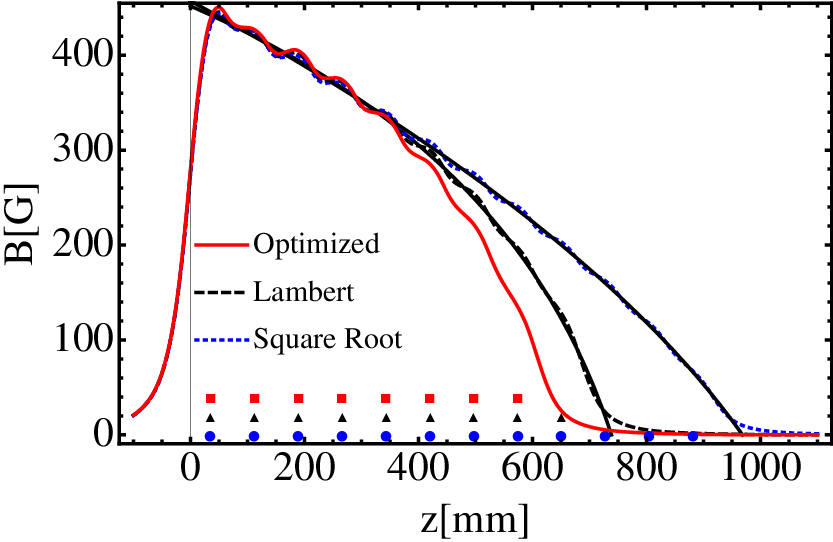
Figure 2 shows the result of optimizing for a fixed slower length of 12 coils compared to the results of fitting to a square root target field and to a Lambert target field, all with with the same maximal noise . The oscillations in the field profile stem from the discrete nature of the system and are taken into account implicitly in the noise parameter. In all cases the adiabatic following condition is satisfied. The optimized maximum field is , corresponding to a capture velocity of , whereas the Lambert field allows , and the traditional (square root) field only permits .
We may also use this method to design a shorter slower. We take for , which is the maximal velocity for a 12-coil slower designed with the traditional field approach to withstand noise of . At this initial velocity we can use the Lambert target field with 9 coils, while still maintaining . When we optimize the system under the constraint,
| (20) |
and the yield function , we arrive at a slower with 8 coils. The results, along with the coil center positions, are shown in Fig. 3.
VI summary
In summary we have introduced two new approaches for the design of a Zeeman slower which rely on optimal compliance with the adiabatic following condition. These approaches allow to optimize system parameters, such as the capture velocity and the slower length.
We have shown that these two approaches yield better results than the traditionally used square-root (constant deceleration) approach. We note that the two approaches are complementary in that the first is useful for the design a system and the second one is useful for optimizing it after some measurements, such as the magnetic field and the noise, have been taken.
VII Acknowledgements
This work was supported by the Israeli Science Foundation under ISF grant 177/11.
References
- [1] M. Gupta and D. Herschbach, The Journal of Physical Chemistry A 105, 1626 (2001).
- [2] J. M. Doyle, B. Friedrich, J. Kim, and D. Patterson, Phys. Rev. A 52, R2515 (1995).
- [3] R. Fulton, A. I. Bishop, and P. F. Barker, Phys. Rev. Lett. 93, 243004 (2004).
- [4] H. L. Bethlem, G. Berden, and G. Meijer, Phys. Rev. Lett. 83, 1558 (1999).
- [5] E. Narevicius, A. Libson, C. G. Parthey, I. Chavez, J. Narevicius, et al., Phys.Rev.Lett. 100, 093003 (2008).
- [6] W. D. Phillips and H. Metcalf, Phys. Rev. Lett. 48, 596 (1982).
- [7] C. Dedman, J. Nes, T. Hanna, R. Dall, K. Baldwin, and A. Truscott, Review of Scientific Instruments 75, 5136 (2004).
- [8] R. Napolitano, S. Zilio, and V. Bagnato, Optics Communications 80, 110 (1990), ISSN 0030-4018.
- [9] J. Tempelaars, J. Tempelaars, J. Tempelaars, and J. Tempelaars, Trapping Metastable Neon Atoms (Technische Universiteit Eindhoven, 2001), ISBN 9789038617596.
- [10] R. Corless, G. Gonnet, D. Hare, D. Jeffrey, and D. Knuth, Advances in Computational Mathematics 5, 329 (1996), ISSN 1019-7168.
- [11] B. Ohayon and G. Ron, To be submitted (2013).
- [12] G. Reinaudi, C. B. Osborn, K. Bega, and T. Zelevinsky, J. Opt. Soc. Am. B 29, 729 (2012).
- [13] P. E. Gill, W. Murray, and M. H. Wright, Practical optimization (Academic Press Inc. [Harcourt Brace Jovanovich Publishers], London, 1981), ISBN 0-12-283950-1.