High-dimensional sequence transduction
Abstract
We investigate the problem of transforming an input sequence into a high-dimensional output sequence in order to transcribe polyphonic audio music into symbolic notation. We introduce a probabilistic model based on a recurrent neural network that is able to learn realistic output distributions given the input and we devise an efficient algorithm to search for the global mode of that distribution. The resulting method produces musically plausible transcriptions even under high levels of noise and drastically outperforms previous state-of-the-art approaches on five datasets of synthesized sounds and real recordings, approximately halving the test error rate.
Index Terms:
Sequence transduction, restricted Boltzmann machine, recurrent neural network, polyphonic transcriptionMontréal (QC), H3C 3J7, Canada
1 Introduction
Machine learning tasks can often be formulated as the transformation, or transduction, of an input sequence into an output sequence: speech recognition, machine translation, chord recognition or automatic music transcription, for example. Recurrent neural networks (RNN) [1] offer an interesting route for sequence transduction [2] because of their ability to represent arbitrary output distributions involving complex temporal dependencies at different time scales.
When the output predictions are high-dimensional vectors, such as tuples of notes in musical scores, it becomes very expensive to enumerate all possible configurations at each time step. One possible approach is to capture high-order interactions between output variables using restricted Boltzmann machines (RBM) [3] or a tractable variant called NADE [4], a weight-sharing form of the architecture introduced in [5]. In a recently developed probabilistic model called the RNN-RBM, a series of distribution estimators (one at each time step) are conditioned on the deterministic output of an RNN [6, 7]. In this work, we introduce an input/output extension of the RNN-RBM that can learn to map input sequences to output sequences, whereas the original RNN-RBM only learns the output sequence distribution. In contrast to the approach of [2] designed for discrete output symbols, or one-hot vectors, our high-dimensional paradigm requires a more elaborate inference procedure. Other differences include our use of second-order Hessian-free (HF) [8] optimization11 1 Our code is available online at http://www-etud.iro.umontreal.ca/~boulanni/icassp2013. but not of LSTM cells [9] and, for simplicity and performance reasons, our use of a single recurrent network to perform both transcription and temporal smoothing. We also do not need special “null” symbols since the sequences are already aligned in our main task of interest: polyphonic music transcription.
The objective of polyphonic transcription is to obtain the underlying notes of a polyphonic audio signal as a symbolic piano-roll, i.e. as a binary matrix specifying precisely which notes occur at each time step. We will show that our transduction algorithm produces more musically plausible transcriptions in both noisy and normal conditions and achieve superior overall accuracy [10] compared to existing methods. Our approach is also an improvement over the hybrid method in [6] that combines symbolic and acoustic models by a product of experts and a greedy chronological search, and [11] that operates in the time domain under Markovian assumptions. Finally, [12] employs a bidirectional RNN without temporal smoothing and with independent output note probabilities. Other tasks that can be addressed by our transduction framework include automatic accompaniment, melody harmonization and audio music denoising.
2 Proposed architecture
2.1 Restricted Boltzmann machines
An RBM is an energy-based model where the joint probability of a given configuration of the visible vector (output) and the hidden vector is:
| (1) |
where , and are the model parameters and is the usually intractable partition function. The marginalized probability of is related to the free-energy by :
| (2) |
The gradient of the negative log-likelihood of an observed vector involves two opposing terms, called the positive and negative phase:
| (3) |
where . The second term can be estimated by a single sample obtained from a Gibbs chain starting at :
| (4) |
resulting in the well-known contrastive divergence algorithm [13].
2.2 NADE
The neural autoregressive distribution estimator (NADE) [4] is a tractable model inspired by the RBM. NADE is similar to a fully visible sigmoid belief network in that the conditional probability distribution of a visible unit is expressed as a nonlinear function of the vector :
| (5) |
| (6) |
where is the logistic sigmoid function.
In the following discussion, one can substitute RBMs with NADEs by replacing equation (4) with the exact gradient of the negative log-likelihood cost :
| (7) |
| (8) |
| (9) |
In addition to the possibility of using HF for training, a tractable distribution estimator is necessary to compare the probabilities of different output sequences during inference.
2.3 The input/output RNN-RBM
The I/O RNN-RBM is a sequence of conditional RBMs (one at each time step) whose parameters are time-dependent and depend on the sequence history at time , denoted where are respectively the input and output sequences. Its graphical structure is depicted in Figure 1. Note that by ignoring the input , this model would reduce to the RNN-RBM [6]. The I/O RNN-RBM is formally defined by its joint probability distribution:
| (10) |
where the right-hand side multiplicand is the marginalized probability of the RBM (eq. 2) or NADE (eq. 5).
Following our previous work, we will consider the case where only the biases are variable:
| (11) |
| (12) |
where are the hidden units of a single-layer RNN:
| (13) |
where the indices of weight matrices and bias vectors have obvious meanings. The special case gives rise to a transcription network without temporal smoothing. Gradient evaluation is based on the following general scheme:
By setting , the I/O-RNN-RBM reduces to a regular RNN that can be trained with the cross-entropy cost:
| (14) |
where and equations (12) and (13) hold. We will use this model as one of our baselines for comparison.
A potential difficulty with this training scenario stems from the fact that since is known during training, the model might (understandably) assign more weight to the symbolic information than the acoustic information. This form of teacher forcing during training could have dangerous consequences at test time, where the model is autonomous and may not be able to recover from past mistakes. The extent of this condition obviously depends on the ambiguousness of the audio and the intrinsic predictability of the output sequences, and can also be controlled by introducing noise to either or , or by adding the regularization terms to the objective function. It is trivial to revise the stochastic gradient descent updates to take those penalties into account.
3 Inference
A distinctive feature of our architecture are the (optional) connections that implicitly tie to its history and encourage coherence between successive output frames, and temporal smoothing in particular. At test time, predicting one time step requires the knowledge of the previous decisions on (for ) which are yet uncertain (not chosen optimally), and proceeding in a greedy chronological manner does not necessarily yield configurations that maximize the likelihood of the complete sequence22 2 Note that without temporal smoothing (), the would be conditionally independent given and the prediction could simply be obtained separately at each time step .. We rather favor a global search approach analogous to the Viterbi algorithm for discrete-state HMMs. Since in the general case the partition function of the RBM depends on , comparing sequence likelihoods becomes intractable, hence our use of the tractable NADE.
Our algorithm is a variant of beam search for high-dimensional sequences, with beam width and maximal branching factor (Algorithm 1). Beam search is a breadth-first tree search where only the most promising paths (or nodes) at depth are kept for future examination. In our case, a node at depth corresponds to a subsequence of length , and all descendants of that node are assumed to share the same sequence history ; consequently, only is allowed to change among siblings. This structure facilitates identifying the most promising paths by their cumulative log-likelihood. For high-dimensional output however, any non-leaf node has exponentially many children (), which in practice limits the exploration to a fixed number of siblings. This is necessary because enumerating the configurations at a given time step by decreasing likelihood is intractable (e.g. for RBM or NADE) and we must resort to stochastic search to form a pool of promising children at each node. Stochastic search consists in drawing samples of and keeping the unique most probable configurations. This procedure usually converges rapidly with samples, especially with strong biases coming from the conditional terms. Note that or reduces to a greedy search, and corresponds to an exhaustive breadth-first search.
Find the most likely sequence under a model with beam width and branching factor .
⋆A min-priority queue of fixed capacity maintains (at most) the highest values at all times.
When the output units are conditionally independent given , such as for a regular RNN (eq. 14), it is possible to enumerate configurations by decreasing likelihood using a dynamic programming approach (Algorithm 2). This very efficient algorithm in is based on linearly growing priority queues, where need not be specified in advance. Since inference is usually the bottleneck of the computation, this optimization makes it possible to use much higher beam widths with unbounded branching factors for RNNs.
Enumerate the most probable configurations of independent Bernoulli random variables with parameters .
denotes the symmetric difference of two sets. indicates the -permutation of indices in the set .
A pathological condition that sometimes occurs with beam search over long sequences () is the exponential duplication of highly likely quasi-identical paths differing only at a few time steps, that quickly saturate beam width with essentially useless variations. Several strategies have been tried with moderate success in those cases, such as committing to the most likely path every time steps (periodic restarts [14]), pruning similar paths, or pruning paths with identical previous time steps (the local assumption), where is a maximal time lag that the chosen architecture can reasonably describe (e.g. for RNNs trained with HF). It is also possible to initialize the search with Algorithm 1 then backtrack at each node iteratively, resulting in an anytime algorithm [15].
4 Experiments
In the following experiments, the acoustic input is constituted of powerful DBN-based learned representations [16]. The magnitude spectrogram is first computed by the short-term Fourier transform using a 128 ms sliding Blackman window truncated at 6 kHz, normalized and cube root compressed to reduce the dynamic range. We apply PCA whitening to retain 99% of the training data variance, yielding roughly dimensionality reduction. A DBN is then constructed by greedy layer-wise stacking of sparse RBMs trained in an unsupervised way to model the previous hidden layer expectation () [17]. The whole network is finally finetuned with respect to a supervised criterion (e.g. eq. 14) and the last layer is then used as our input for the spectrogram frame at time .
We evaluate our method on five datasets of varying complexity: Piano-midi.de, Nottingham, MuseData and JSB chorales (see [6]) which are rendered from piano and orchestral instrument soundfonts, and Poliner & Ellis [18] that comprises synthesized sounds and real recordings. We use frame-level accuracy [10] for model evaluation. Hyperparameters are selected by a random search [19] on predefined intervals to optimize validation set accuracy; final performance is reported on the test set.
| Dataset | HMM [16] | RNN-RBM [6] | Proposed |
|---|---|---|---|
| Piano-midi.de | 59.5% | 60.8% | 64.1% |
| Nottingham | 71.4% | 77.1% | 97.4% |
| MuseData | 35.1% | 44.7% | 66.6% |
| JSB Chorales | 72.0% | 80.6% | 91.7% |
Table 1 compares the performance of the I/O RNN-RBM to the HMM baseline [16] and the RNN-RBM hybrid approach [6] on four datasets. Contrarily to the product of experts of [6], our model is jointly trained, which eliminates duplicate contributions to the energy function and the related increase in marginals temperature, and provides much better performance on all datasets, approximately halving the error rate in average over these datasets.
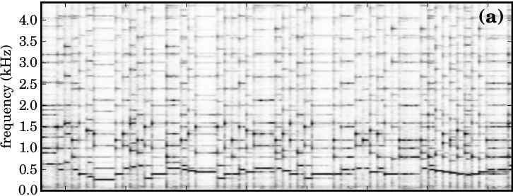


We now assess the robustness of our algorithm to different types of noise: white noise, pink noise, masking noise and spectral distortion. In masking noise, parts of the signal of exponentially distributed length ( s) are randomly destroyed [20]; spectral distortion consists in Gaussian pitch shifts of amplitude [21]. The first two types are simplest because a network can recover from them by averaging neighboring spectrogram frames (e.g. Kalman smoothing), whereas the last two time-coherent types require higher-level musical understanding. We compare a bidirectional RNN [12] adapted for frame-level transcription, a regular RNN with connections () and the I/O RNN-NADE (). Figure 2 illustrates the importance of temporal smoothing connections and the additional advantage provided by conditional distribution estimators. Beam search is responsible for a 0.5% to 18% increase in accuracy over a greedy search ().
Figure 3 shows transcribed piano-rolls for various RNNs on an excerpt of Bach’s chorale Es ist genug with 6 dB pink noise (Fig. 3(a)). We observe that a bidirectional RNN is unable to perform temporal smoothing on its own (Fig. 3(b)), and that even a post-processed version (Fig. 3(c)) can be improved by our global search algorithm (Fig. 3(d)). Our best model offers an even more musically plausible transcription (Fig. 3(e)). Finally, we compare the transcription accuracy of common methods on the Poliner & Ellis [18] dataset in Table 2, that highlights impressive performance.
5 Conclusions
We presented an input/output model for high-dimensional sequence transduction in the context of polyphonic music transcription. Our model can learn basic musical properties such as temporal continuity, harmony and rhythm, and efficiently search for the most musically plausible transcriptions when the audio signal is partially destroyed, distorted or temporarily inaudible. Conditional distribution estimators are important in this context to accurately describe the density of multiple potential paths given the weakly discriminative audio. This ability translates well to the transcription of “clean” signals where instruments may still be buried and notes occluded due to interference, ambient noise or imperfect recording techniques. Our algorithm approximately halves the error rate with respect to competing methods on five polyphonic datasets based on frame-level accuracy. Qualitative testing also suggests that a more musically relevant metric would enhance the advantage of our model, since transcription errors often constitute reasonable alternatives.
References
- [1] D.E. Rumelhart, G.E. Hinton, and R.J. Williams, “Learning internal representations by error propagation,” in Parallel Dist. Proc., pp. 318–362. MIT Press, 1986.
- [2] A. Graves, “Sequence transduction with recurrent neural networks,” in ICML 29, 2012.
- [3] P. Smolensky, “Information processing in dynamical systems: Foundations of harmony theory,” in Parallel Dist. Proc., pp. 194–281. MIT Press, 1986.
- [4] H. Larochelle and I. Murray, “The neural autoregressive distribution estimator,” JMLR: W&CP, vol. 15, pp. 29–37, 2011.
- [5] Y. Bengio and S. Bengio, “Modeling high-dimensional discrete data with multi-layer neural networks,” in NIPS 12, 2000, pp. 400–406.
- [6] N. Boulanger-Lewandowski, Y. Bengio, and P. Vincent, “Modeling temporal dependencies in high-dimensional sequences: Application to polyphonic music generation and transcription,” in ICML 29, 2012.
- [7] I. Sutskever, G. Hinton, and G. Taylor, “The recurrent temporal restricted Boltzmann machine,” in NIPS 20, 2008, pp. 1601–1608.
- [8] J. Martens and I. Sutskever, “Learning recurrent neural networks with Hessian-free optimization,” in ICML 28, 2011.
- [9] S. Hochreiter and J. Schmidhuber, “Long short-term memory,” Neural Computation, vol. 9, no. 8, pp. 1735–1780, 1997.
- [10] M. Bay, A.F. Ehmann, and J.S. Downie, “Evaluation of multiple-F0 estimation and tracking systems,” in ISMIR, 2009.
- [11] A.T. Cemgil, H.J. Kappen, and D. Barber, “A generative model for music transcription,” IEEE Transactions on Audio, Speech, and Language Processing, vol. 14, no. 2, pp. 679–694, 2006.
- [12] S. Böck and M. Schedl, “Polyphonic piano note transcription with recurrent neural networks,” in ICASSP, 2012, pp. 121–124.
- [13] G.E. Hinton, “Training products of experts by minimizing contrastive divergence,” Neural Computation, vol. 14, no. 8, pp. 1771–1800, 2002.
- [14] S. Richter, J.T. Thayer, and W. Ruml, “The joy of forgetting: Faster anytime search via restarting,” in ICAPS, 2010, pp. 137–144.
- [15] R. Zhou and E.A. Hansen, “Beam-stack search: Integrating backtracking with beam search,” in ICAPS, 2005, pp. 90–98.
- [16] J. Nam, J. Ngiam, H. Lee, and M. Slaney, “A classification-based polyphonic piano transcription approach using learned feature representations,” in ISMIR, 2011.
- [17] Y. Bengio, “Learning deep architectures for AI,” Foundations and Trends in Machine Learning, vol. 2, no. 1, pp. 1–127, 2009.
- [18] G.E. Poliner and D.P.W. Ellis, “A discriminative model for polyphonic piano transcription,” JASP, vol. 2007, no. 1, pp. 154–164, 2007.
- [19] J. Bergstra and Y. Bengio, “Random search for hyper-parameter optimization,” Journal of Machine Learning Research, vol. 13, pp. 281–305, 2012.
- [20] P. Vincent, H. Larochelle, Y. Bengio, and P.A. Manzagol, “Extracting and composing robust features with denoising autoencoders,” in ICML 25, 2008, pp. 1096–1103.
- [21] K.J. Palomäki, G.J. Brown, and J.P. Barker, “Techniques for handling convolutional distortion with ‘missing data’ automatic speech recognition,” Speech Communication, vol. 43, no. 1, pp. 123–142, 2004.
- [22] M. Marolt, “A connectionist approach to automatic transcription of polyphonic piano music,” IEEE Transactions on Multimedia, vol. 6, no. 3, pp. 439–449, 2004.
- [23] M.P. Ryynänen and A. Klapuri, “Polyphonic music transcription using note event modeling,” in ASPAA, 2005, pp. 319–322.
- [24] C.G. Boogaart and R. Lienhart, “Note onset detection for the transcription of polyphonic piano music,” in ICME, 2009, pp. 446–449.