Binding of an oxide layer to a metal: the case of Ti(100)/TiO2(100)
Abstract
We study the chemical nature of the bonding of an oxide layer to the parent metal. In order to disentangle chemical effects from strain/misfit, Ti(100)/TiO2(100) interface has been chosen. We use the density functional pseudopotential method which gives good agreement with experiment for known properties of bulk and surface Ti and TiO2. Two geometries, a film-like model (with free surface in the structure) and a bulk-like model (with no free surface in the structure) are used to simulate the interface, in each case with different terminations of Ti and TiO2. For the single-oxygen interfaces, the interface energy obtained using these two models agree with each other; however for the double-oxygen ones, the relative stability is quite different. The disturbance to the electronic structure is confined within a few atomic layers of the interface. The interfacial bonding is mainly ionic, and surprisingly there is more charge transfer from Ti to O in the interface than in the bulk. In consequence the Ti/TiO2 interface has stronger binding than the bulk of either material. This helps to explain why the oxide forms a stable, protective layer on Ti and Ti alloys.
1 INTRODUCTION
In contrast to the many atomistic studies of metals and oxides, both at the ab initio and empirical level, the metal-oxide interface is much less well studied. This may appear surprising given its central role in corrosion. One reason may be the difficulty in identifying a candidate interface where the chemical effects are not entangled with misfit strain energy. Another is the relatively large size of system which is required to isolate the system. Although the strain energy is long-ranged, there are reasons to expect that the chemical effects of the interface may not be: on the metal side the free electrons should screen the Coulomb forces, while the image charges induced in the metal should mimic the electrostatics of a bulk oxide. At the interface itself, such classical ideas break down, and a full quantum treatment is needed to determine the nature of the bonding. In this paper we will consider the low-misfit Ti(100)/TiO2(100) interface, with a view to determining the range over which chemical effects are significant and the nature of the bonding cross the interface.
Titanium alloys are widely used in many fields such as the aerospace industry, chemical plants, and even sporting goods. The high strength-to-weight ratio and excellent corrosion resistance account for its wide application. The corrosion property is mainly a result of the formation of stable protective oxide film, which consists primarily of TiO2. However, above 600∘C, the fast diffusion of oxygen through the oxide layer into the bulk can result in excessive growth of oxide layer and embrittlement of the adjacent oxygen rich layer of the titanium alloy, which limits its maximum use temperature.Lutjering and Williams (2007) Alloying and coating have been found effective to address this problem. Obviously, the interface between the titanium and its oxide plays a vital role in the corrosion, both through its adhesive strength and the diffusion of species (O and/or Ti) through it, and its structure is a key aspect for understanding the behavior of titanium alloys.
Extensive experiments on pure titaniumFlower and Swann (1974); Kozlowski et al. (1988); Ting et al. (2002); Kumar et al. (2010) and titanium alloysLopez et al. (2003); Garcia-Alonso et al. (2003) have established that the crystal structure of the oxide is normally rutile (tetragonal, P42/mnm). Although Guleryuz et al.Guleryuz and Cimenoglu (2004) reported some diffraction angles consistent with the anatase structure(tetragonal, I41/amd), in the scale of Ti-6Al-4V oxidized at 600∘C, rutile is the dominant oxide at 650∘C. Due to the competition between surface free energy and strain energy, the growth of rutile on pure titanium exhibits a preferential direction,Kozlowski et al. (1988); Ting et al. (2002) with a specific crystallographic orientation relationship (COR) between titanium and rutile. Three possible CORs between Ti and rutile were established by Flower et al.Flower and Swann (1974) using an in situ method: Ti(0001)[110] // TiO2(010)[001], Ti(100)[0001] // TiO2(100)[010] and Ti(110)[0001] // TiO2(001)[100]. Among these three different matchings, Ti(100)[0001] // TiO2(100)[010] has the smallest mismatch on the plane of the interface, which means only a tiny interface strain would be required.
The structure of the oxide and the orientation relationship can be easily determined by the experiments; however, some other quantities like the chemical composition, atomic structure of the interface, and the nature of the bonding (ionic/metallic/covalent) across the interface are currently experimentally inaccessible. Fortunately, nowadays, it is possible to deal with coherent interface structures (large system, low symmetry) using accurate first-principles theoretical methods to obtain those quantities. Coherency implies that one part (metal or oxide) will be strained to match the other one perfectly to maintain the coherency without misfit dislocations. In this case, DFT supercell method can be a good tool to study interfaces with small mismatch, but even when the misfit is quite big, it has been assumed that the interfacial regions between the misfit dislocation being modelled.Siegel et al. (2002) Such a first-principles supercell method has been used to study many different interfaces, for example, interface of ZrO2/Ni,Christensen and Carter (2001) Al/Al2O3,Siegel et al. (2002) Ti/TiN,Liu et al. (2003) YSZ/Al2O3,Lallet et al. (2009) Nb/Nb5Si3,Shang et al. (2010) etc. Here we present a DFT study of Ti(100)[0001] // TiO2(100)[010] interface. The purpose of this study is to determine the optimal atomic structure and energy of Ti(100)[0001] // TiO2(100)[010] interface, and characterize the nature of the interfacial bonding.
2 METHODS
The Vienna Ab initio Simulation Package (VASP)Kresse and Hafner (1993); Kresse and Furthmüller (1996); G. and J. (1996) utilizing a plane-wave basis set for the expansion of the single-particle Kohn-Sham wave functions, was used in this study. The projector augmented wave (PAW) methodBlöchl (1994), was employed to describe the electron-core interaction. The 3p semicore electrons of Ti were treated as valence, given a 10-electron PAW-pseudopotential. For the exchange-correlation interaction, we adopted generalized gradient approximation (GGA) as parameterized by Perdew and Wang (PW91).Perdew and Wang (1992) A high cutoff energy of 525 eV was used. Sampling of the Brillouin zone was performed with a Monkhorst-Pack grid.Monkhorst and Pack (1976) Ground-state atomic structures were obtained by minimizing the Hellmann-Feynman forces on the atoms, and all the atoms were free to relax. The relaxations terminate when the maximum force on the atoms is less than 0.05 eV/Å. For some calculations a dipole moment is present, in such cases the divergent terms are removed by the Ewald sum; we did not include a dipole correctionBengtsson1999 as previous work in TiO2 has shown this to have minor effects.
3 RESULTS: parameters and basic properties of Ti and TiO2
3.1 Bulk properties
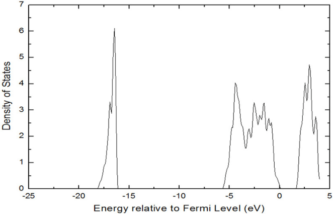
To verify the accuracy of our computational parameters, we first calculated the bulk properties of Ti and rutile. The k-point mesh was set at and for the bulk TiO2 and hcp-Ti, respectively. These provide convergence to within 1 meV and as can be seen from 1 the calculated lattice parameter and bulk modulus data agree excellently with the experiments. From the DOS of TiO2 (1), the gap between highest occupied and lowest unoccupied state of TiO2 is about 1.7 eV, far away from the experimental value, which is around 3.0 eVGRANT (1959): this does not affect the bonding and is typical of the error of DFT in describing excited states.
3.2 Surface properties
To determine the minimum slab thickness needed to reliably calculate the surface/interface we examined the convergence of the relaxation and energy of the surfaces with respect to slab thickness. In this calculation, we used k-point sampling and for Ti(100) and TiO2(100). In both slabs, a 15 Å vacuum region is introduced to avoid the interaction between periodic images. For both surfaces, only the (1 1) structures (along the two lattice vectors of the surface, the symmetry is the same as in the bulk) are considered, since these have been observed by for clean surface under normal conditions by experimentalists.III and Watson (1989); III and Watson (1989); Diebold (2003)
The calculated surface energy might diverge with the thickness of the slab, if there is any numerical difference between the calculation of bulk and slab, arising, for example, from the k-point mesh. Following BoettgerBoettger (1994) we avoid this possibility, by evaluating the surface energy as follows:
| (1) |
where is the minimum number of the slab layers for which the energy converges, is the energy of a N-layer slab, and S is the area of the surface.
3.2.1 Ti(100)
In hcp Ti, two different (100) planes exist, depending on whether the surface terminates in a large (1.694 Å) or small (0.847 Å) interlayer spacing. From the experimental results, III and Watson (1989) Ti(100) surface with a small first interlayer spacing was the favored one. Our calculation confirmed this, and henceforth, we concentrate on the more stable Ti(100) surface.
| Layer | ||||||||
|---|---|---|---|---|---|---|---|---|
| 12 | -3.26 | -5.43 | 5.98 | -2.20 | 3.65 | 1.99 | ||
| 14 | -3.64 | -4.74 | 4.10 | -1.13 | 2.19 | 2.16 | 1.99 | |
| 16 | -3.75 | -4.80 | 3.95 | -1.01 | 1.97 | 1.25 | -0.29 | 1.99 |
| 18 | -3.70 | -4.93 | 3.99 | -1.18 | 2.07 | 1.39 | -0.39 | 1.99 |
| Expt.a | -5.9 |
a ref 24
The surface relaxation data is shown in 2, the distance between the first two layers decreases by about 4% compared with that in the bulk, in reasonable agreement with 6% from the experiment III and Watson (1989) (the discrepancy is less than 0.02 Å). contracts and expands, showing the same trend as the results by self-consistent tight bonding model.Erdin et al. (2005) Relaxations between deeper layers are even smaller (less than 2%). The surface energy converged quickly with cell size to 1.99 J/m2. This is slightly higher than the 1.91 J/m2 of Ti(0001) surface which we obtained using the same method: Ti(0001) has an experimental energy of 1.99 J/m2.Tyson and Miller (1977) Thus Ti(100) is just slightly less stable than the close-packed Ti(0001) surface. For further study, we chose a 16-layer slab to simulate Ti(100).
3.2.2 TiO2(100)
Extensive theoretical studies have been done to investigate the TiO2(100) surfaces. There are three possible terminations for TiO2(100), which we call O-Ti-O, O-O-Ti, and Ti-O-O (named by the atomic arrangement from the surface to inner layer). The first of these (2) has the smallest surface polarization due to the symmetrical arrangement of O, and the geometry has been observed by experiment.Diebold (2003) We find it to be the most stable one, and we use the O-Ti-O terminated TiO2(100) surface to determine the minimum thickness of the slab needed. One thing that should be noted is that in this subsection, the O-Ti-O unit is treated as one layer, i.e., the 5-layer slab mentioned here has 15 atomic layers.
The choice of exchange-correlation functional has been found to affect the surface energy quite significantly,Muscat et al. (1999) and normally LDA gives a higher surface energy than GGA. Due to the lack of the experimental results, it is difficult to clarify which function best describes the real situation. Here, we compared our results with other calculations using the same exchange-correlation function (GGA), in order to verify the accuracy of our calculation. As shown in 3, O1, Ti2, and O3 exhibit large relaxations along [00]. Moreover, Ti2 relaxes inward along [100], while outward relaxation is observed for O1 and O3. These relaxations increase the effective coordination of Ti2 (fivefold).Muscat et al. (1999); Labat et al. (2008) Our surface relaxation results agree with that found by Muscat et al..Muscat et al. (1999) 4 lists the surface energy dependence on the slab thickness: it converges quickly to 0.68 J/m2 which agrees very well with Perron et al. Perron et al. (2007) (10 valence electrons are considered for Ti) and Labat et al. (GGA-PBE),Labat et al. (2008) while it is smaller than Muscat’s GGA resultMuscat et al. (1999). Considering the convergence of both the surface structure and energy, we believe that a 13-layer slab is thick enough to model TiO2(100).

| 5 | 9 | 13 | 17 | Ref.a | ||||||
|---|---|---|---|---|---|---|---|---|---|---|
| Label | [00] | [100] | [00] | [100] | [00] | [100] | [00] | [100] | [00] | [100] |
| 1 | 0.32 | 0.07 | 0.32 | 0.08 | 0.28 | 0.06 | 0.28 | 0.06 | 0.31 | 0.06 |
| 2 | -0.10 | -0.03 | -0.11 | -0.02 | -0.15 | -0.03 | -0.15 | -0.03 | -0.11 | -0.04 |
| 3 | 0.17 | 0.06 | 0.18 | 0.08 | 0.14 | 0.06 | 0.13 | 0.05 | 0.13 | 0.02 |
| 4 | 0.07 | 0.01 | 0.08 | 0.02 | 0.04 | 0.01 | 0.04 | 0.00 | 0.03 | 0.00 |
| 5 | -0.05 | 0.02 | -0.06 | 0.04 | -0.10 | 0.03 | -0.10 | 0.02 | ||
| 6 | 0.01 | 0.03 | 0.04 | 0.04 | 0.00 | 0.02 | 0.00 | 0.02 | ||
| 7 | 0.01 | -0.01 | 0.04 | 0.01 | 0.01 | -0.01 | 0.01 | -0.01 | ||
aref 29.
4 RESULTS: Interface properties
The orientation relationship is set as Ti(100)[0001] // TiO2(100)[010] across the interface. The size of the Ti(100) surface cell is 2.934 Å 4.638 Å, while it is 2.971 Å 4.645 Å for TiO2(100). A coherent interface is obtained by a small strain of the softer Ti to perfectly match the TiO2(100) surface cell: this has little effect on the energy since the mismatch of the two surface cells is so small. To check dependence on boundary conditions we used two models to simulate the interface, a film-like model with an interface and two free surfaces, and a bulk-like model with two interfaces. The interface structures were relaxed with k-point mesh (four irreducible k points).
4.1 Film-like interface model
The film-like model is generated with 16-layers of Ti, 13-layers of TiO2 and a 15 Å vacuum region. This gives one interface and two free surfaces.
Various terminations of the surfaces and metal/oxide interface are possible, their stability depending on the environmental condition like the partial pressure of O2 gas.Zhang and Smith (2000) As we mentioned above, TiO2(100) has three possible terminations, with uppermost layers O-O-Ti, O-Ti-O, and Ti-O-O. For interfaces, we considered different stacking sequences of Ti onto these terminations. Following work on other interfacesSiegel et al. (2002); Liu et al. (2003), the first layer of the Ti-metal is placed…
- •
’OT’: directly above uppermost Ti cations;
- •
’HCP’: above the second layer of Ti cations;
- •
’FCC’: above the third layer of Ti cations.
- •
’TT’: for O-O-Ti, as an extension of the oxide.
- •
’TT’: for Ti-O-O, as an extension of the metal.
The ’TT’ configurations are those which would allow growth of the oxide/metal by simple extension of a stable interface, with the Ti ’atoms’ and Ti ’cations’ directly adjacent. In fact, the two ’TT’ configurations are the same at the interface, the calculation differing in the accompanying surface.
Despite this apparently exhaustive survey of stacking sequences, we also found that where the TiO2(100) surface is quite corrugated, significant reconstruction can occur within the Ti-metal region, spontaneously generating a stacking fault. When this happens, we report the most stable relaxed structure, and label it ’HCP-2’ and ’FCC-2’ in 5.
To avoid spurious contraction due to surface tension, we fix the lattice parameters in the interface plane. But we allow relaxation perpendicular by first calculating the total energy of the unrelaxed interface structure as a function of interface separations . Once the optimal value is found, all the atoms are relaxed to the ground state at fixed volume.
In order to evaluate the strength of the interface, we calculated the work of adhesion, , which is defined as:
where is the surface energy of Ti-metal, is the surface energy of oxide, is the energy of the interface structure, and S is the interface area. A positive value of means that the interface is energetically favorable over the free surfaces. 5 shows that increases with increasing number of interfacial O atoms (Ti-O-O, O-Ti-O, and O-O-Ti). However, much of this is due to differences in surface stability; e.g. the O-O-Ti and Ti-O-O with ’TT’ stacking have the same chemical composition near the interface but very different .
To understand the growth of an additional TiO2 layer, each of these interface types needs to be considered. In the following subsections, the interface with the most stable stacking sequence for each termination is analyzed in detail.
| O-O-Ti | O-Ti-O | Ti-O-O | |||||||||||
|---|---|---|---|---|---|---|---|---|---|---|---|---|---|
| OT | HCP | FCC | TT | HCP-2 | OT | HCP | FCC | FCC-2 | OT | HCP | FCC | TT | |
| d | 1.65 | 0.57 | 1.09 | 0.97 | 1.17 | 1.87 | 1.37 | 0.33 | 0.31 | 1.90 | 1.66 | 1.58 | 0.55 |
| 7.54 | 9.43 | 8.99 | 9.32 | 10.34 | 2.28 | 2.57 | 3.49 | 3.55 | 1.41 | 2.59 | 2.04 | 2.83 | |
For all configurations listed in 6, for the metal slab, the Ti atom in the center has a charge 0.00, as in bulk Ti, which again confirms that the slab we used is thick enough. For the TiO2 slab, the charge associated with central Ti and O ions are 2.18e and -1.10e, respectively. This agrees well with DFT results from Jess and the co-workersller et al. (2010) who found the Bader charge is 2.22e and -1.12e for Ti and O. Although Bader charge values are far from the formal charge 4e (Ti4+) and -2e (O2-), we believe that useful bonding information can be obtained from the charge transfer.
4.1.1 Atomic, electronic structure of O-O-Ti interface

The stacking sequence ’HCP-2’ gives rise to the most stable O-O-Ti interface (5). The structure is displayed in 3. To observe the geometry change due to the atomic relaxation clearly, the unrelaxed (input) structure is also shown and the ions with large displacement are labeled. On the metallic side, Ti2 and Ti4 move towards the oxide. Ti1 and Ti2 are found shifting along [000] of Ti significantly. As a result, the surface morphology of Ti(100) is totally changed: the Ti1 and Ti2 layers merge to give a flat surface; the spacing between Ti2 and Ti3 layer changes to 2.19 Å from 1.69 Å in the bulk; the interlayer spacing between Ti3 and Ti4 decreases to 0.43 Å from the bulk spacing 0.85 Å. For the oxide slab, the relaxation is less significant, the interfacial atoms move towards metal slab, in particularly O2, thus the surface of the oxide becomes flatter. Across the interface, the separations of Ti1-O1 and Ti2-O2 is 2.00 Å and 2.15 Å, which is close to the Ti-O bond lengths in bulk TiO2 (1.96 Å and 2.00 Å). O2 is located in the center of the ’half’ octahedron (formed by Ti1, Ti2 and Ti5), and O1 sits in a similar octahedral site.
Bader charge analysisTang et al. (2009) is applied to study the charge transfer. In 6, we give the Bader charge associated with the labeled atoms (3) as well as the atoms in the center of the metal/oxide slabs, and the value of the charge is the variation from the neutral Ti/O atom (10e for Ti, and 6e for O). Thus a negative value means accepting negatively charged electrons, while a positive value means donating electrons.
| Ti slab | TiO2 slab | |||||||
|---|---|---|---|---|---|---|---|---|
| Atom | Ti1 | Ti2 | Ti3 | Ti4 | Ti5 | O1 | O2 | O(center) |
| O-O-Ti film(HCP-2) | 0.81 | 0.82 | -0.21 | 0.32 | 2.08 | -1.20 | -1.28 | -1.11 |
| O-Ti-O film(FCC-2) | 0.82 | 0.06 | 0.24 | 0.01 | 1.78 | -1.37 | -1.24 | -1.10 |
| Ti-O-O film(TT) | 0.56 | -0.06 | 0.18 | -0.04 | 1.12 | -1.27 | -1.20 | -1.09 |
| S-Oa bulk(FCC) | 0.77 | 0.15 | 0.23 | -0.09 | 1.78 | -1.39 | -1.24 | -1.11 |
| D-Ob symmetry bulk(TT) | 1.05 | 0.62 | -0.01 | 0.12 | 2.10 | -1.21 | -1.27 | -1.11 |
| D-Ob asymmetry bulk(TT) | 1.06 | 0.60 | -0.05 | 0.15 | 2.11 | -1.27 | -1.21 | -1.11 |
| D-Ob asymmetry bulk(HCP-2) | 0.83 | 0.81 | -0.19 | 0.31 | 2.08 | -1.19 | -1.28 | -1.11 |
a Single-Oxygen; b Double-oxygen.
For ’HCP-2’ each of the interfacial atoms Ti1 and Ti2 donates 0.8 electrons, which account for the net charge transfer of 1.61 electrons from the metal slab to the oxide (6). Bader analysis gives a negative charge for Ti3, but this appears to be an artifact due to the large relaxation around it, leading to a large Bader volume, which in turn encloses more electrons. It is better to consider the layer containing Ti3 and Ti4, which has overall a small positive charge. The interfacial oxygen ions O1 and O2 attract more electronic charge than the oxygen in the center, due to the more electron donators nearby. Ti5 transfers fewer electrons than the Ti ions in the center of the oxide, which is also understandable as its coordination is smaller. The large electron transfer found here implies strong ionic bonding across the interface.
The electronic density of states is projected onto selected atoms to determine the bonding character (4). Notably, Ti3 and Ti4 are dissimilar, as is reflected in the peak/valley just below the Fermi level. The interfacial atoms Ti1 and Ti2 show a small hybridization peak in the region from -7.5 eV to -2.5 eV, representing weak covalent bonding to the oxygen nearby. Strong hybridization between the Ti and O is observed from the DOS of all ions on the TiO2 side of the interface, indicating some covalent bonding in rutile.Paxton and Thiên-Nga (1998) Ti5 has almost no Ti conduction band density: which implies that bonding in the O-O-Ti structure is not metallic. The DOS of O1 and O2 are similar to the oxygen in the center of oxide slab, with a small shift of both s and p peaks to a lower energy level indicating a stronger Madelung field at the interface, which can stabilize the system.Landa et al. (2009) For the oxygen on the surface, the s orbital shows no shift, and the width of its p orbital is reduced. By comparing the total DOS of the interface slab (5(a)) and DOS of pure TiO2 (1), we see a small peak around -7.5 eV induced by the interface atoms. This will be discussed further later.


4.1.2 Atomic, electronic structure of O-Ti-O interface

As shown in 5, for O-Ti-O interface systems, the interface with strongest adhesion is ’FCC-2’, which has a similar structure to ’FCC’. 6 shows the optimized ’FCC-2’ interface: Ti1 and Ti3 are shifted significantly toward the oxide, forming planes containing both Ti and O atoms. With this displacement, the interlayer spacing of the metal slab near the interface changed to 1.19 Å and 1.36 Å, which are 0.85 Å and 1.69 Å in the bulk Ti, respectively. Relaxation of O1 and O2 leads to a displacement towards the metal even larger than that in the free surface structure. Finally, the separation O1-Ti2 and O2-Ti1 is 2.13 Å and 2.10 Å, close to the spacing in bulk TiO2 (1.96/2.00 Å).
The Bader charge analysis results are listed in 6. The most significant charge transfer comes from Ti1 and Ti3, which donate a total of 1.16 electrons from the metal to the oxide. The excess charge is located on the interfacial atoms (Ti5, O1 and O2).
As seen from 7, the atom-projected DOS converges rapidly to bulklike values away from the interface. For the interfacial ion Ti5, states in the band gap of the oxide implies a kind of metallic behavior, and it is a little stronger than that in O-O-Ti interface, because of its direct exposure to the metal slab. The shift of DOS is very apparent in the interfacial atoms O1 and O2, especially for O1, the 2s states is below -20 eV. For the surface oxygen, the 2s and 2p orbitals move to a higher energy level, which contribute to the small peak near -17.5 eV in the total DOS (5(b)). Also, comparing 1 (pure TiO2), 5(b) (interface with surface), and 5(d) (interface with no surface), it can be concluded that, in 5(b), the small peak below -20 eV and peak near -7.5 eV are associated with the interface atoms, while the peak near -17.5 eV comes from surface atoms. These agree with the our calculation results that the formation of the interface is exothermic, while that is endothermic for the surface.

4.1.3 Atomic, electronic structure of Ti-O-O interface

For the Ti-O-O structures, ’TT’ stacking exhibits the lowest energy. The input and relaxed structure of ’TT’ stacking are shown in 8. Again, the relaxation tends to flatten the surfaces. The interfacial spacing (distance between Ti1 layer and Ti5 layer) is 0.55 Å, smaller than the 0.85 Å of the interlayer spacing in bulk Ti. O1 moves towards the interface, which increases the effective coordination of Ti5. The downward shift of Ti1 and Ti3 are also observed. The interlayer spacing of Ti1-Ti2 and Ti2-Ti3 is 1.88 Å and 0.74 Å, respectively, which slightly deviate from the spacing in the bulk Ti.
The Bader charge analysis (6) and DOS projection (9) are qualitatively similar to the two systems. However, only 0.41e is moved to the oxide slab from the metal, much less than in the other two surfaces. From the projected DOS of the interfacial ions (Ti1,Ti2, Ti3 and Ti4), no covalent features are evident between the two slabs, but metallic bonding can be inferred from the occupied 4s3d states in Ti5 which is adjacent to the metal slab. The relatively small of the Ti-O-O systems can be understood by the pDOS (9), where the 2s states of surface oxygen move to a very high level just below -15 eV. Thus the states between -15 eV and -17.5 eV in the 5(c) come from the oxygen near the free surface (O-O-Ti terminated) included in the slab model.

4.2 Bulk-like interface model
In this model, we consider a periodic arrangement metal-oxide-metal, with no free surfaces. One advantage of this model over the previous one is that the effects of surface dipole interactions are eliminated.
Considering the termination of TiO2(100) at the interface, there are two structures with different layer ordering
- •
Ti-Ti-Ti-O-Ti-O-O-TiO-O-Ti-O-Ti-Ti-Ti,
- •
Ti-Ti-Ti-O-O-Ti-O-O-TiO-O-Ti-O-O-Ti-Ti-Ti.
The former, denoted as single-oxygen interface, may have either two identical interfaces or different stacking sequences. For the latter, double-oxygen interface, we first calculate a ’TT’ configuration where the first cation (metal) layer is like the extension of the metal (oxide). Subsequently we made an ’asymmetric’ structure: one interface with ’TT’ stacking, the other with ’HCP-2’ stacking, so that the energy of the double-oxygen interface with ’HCP-2’ stacking can be obtained. Again, we fix the dimensions of the cell in the interface plane.
In order to evaluate the strength of the interface, we defined the interface energy as:
where is the energy of interface structure consisting of m Ti atoms and n O atoms. is the energy per TiO2 unit in the bulk oxide, is the energy per Ti atom in the bulk metal, and 2S is the area of the two interfaces in the interface structure.
The results are summarized in 8. The negative values indicate that the interface is favored relative to the bulk. In contrast to the results for the O-O-Ti terminated interface shown in 5, ’HCP-2’ stacking here is less stable than the ’TT’ stacking by about 0.1 J/m2.
To illustrate the possible effect of the free surface on the obtained by the film-like model, in 10, we display the structure of the Ti-O-O free surface from the film-like interface slab with ’TT’ and ’HCP-2’ stacking, compared with its structure in the pure TiO2(100) calculation. After relaxation in the surface slab (10(b)), O1 and O2 move significantly outwards, and finally, the Ti-O-O termination transforms to an arrangement like O-Ti-O. In TiO2, the surface terminated with Ti is highly polar and this outward movement of oxygen can decrease the dipolar moment. Very similar relaxation is observed in the interface with ’HCP-2’ stacking (10(d)). However, for the ’TT’ stacking (10(c)), the relaxation of O1 and O2, does not occur, and the termination remains Ti-O-O. As we mentioned above, in ’TT’ stacking, the first Ti layer of the metal sits in a position like the extension of the oxide, so the O-O-Ti terminated interface with a stoichiometric oxide can also be seen as a Ti-O-O terminated interface with a non-stoichiometric oxide. This different surface relaxation directly affects the work of adhesion of the interface. We do not think this kind of interaction between the interface and polarized surface can be removed by increasing the thickness of the oxide slab.

| surface TiO2 unit | inside TiO2 unit | |||||
|---|---|---|---|---|---|---|
| Atom | Ti1 | O1 | O2 | Ti2 | O3 | O4 |
| free surface | 1.94 | -1.03 | -1.19 | 1.88 | -1.23 | -1.13 |
| TT stacking | 1.56 | -1.20 | -1.16 | 2.11 | -1.14 | -1.10 |
| HCP-2 stacking | 1.93 | -1.04 | -1.19 | 1.88 | -1.25 | -1.14 |
In order to analyze the effects of interfaces on the Ti-O-O surface in detail, we examine the Bader charge on the ions near the surface in 7. In all cases the electron density near the surface is enhanced by almost one electron per surface cell. The charge distribution near the free surface is unaffected by an ’HCP-2’ interface, but the presence of a ’TT’ interface, changes the surface charge distribution significantly. This interaction between surface and interface cast doubt on the validity of the film-like model. Similar calculations for the single-oxygen structures (terminated with O-Ti-O), show no such structure or Bader charge variation. Thus for the double-oxygen interface, the film-like model is still reliable.
So get an estimate of finite size error, we can directly compare the calculated work of adhesion for the same interface obtained by bulk-like and film-like calculation (5),and this requires subtraction of the energy of the free surfaces. These are: 1.99 J/m2 and 2.20 J/m2 for Ti(100) terminated with small and large interlayer spacing respectively; 0.68 J/m2 for TiO2(100) terminated with O-Ti-O, and 7.91 J/m2 for the sum of Ti-O-O and O-O-Ti terminations. The resultant interface energy is listed in 8. For the single-oxygen interfaces, is in reasonable agreement with . For the double-oxygen interface with ’TT’ stacking the apparent discrepancy is obviously due to the different surface reconstruction, as just described. And the bulk-like model is more reasonable. In the next subsections, we will discuss the geometry as well as the electronic structure difference for these two models.
| Termination | single-oxygen | double-oxygen | ||||
|---|---|---|---|---|---|---|
| Stacking | OT | HCP | FCC | FCC-2 | TT | HCP-2 |
| 0.30 | -0.03 | -0.95 | -0.93 | -0.60 | -0.51 | |
| 0.39 | 0.10 | -0.82 | -0.88 | -0.05 | ||
4.2.1 Atomic, electronic structure of single-oxygen interface

The structure of ’FCC’ (11) is quite similar as the ’FCC-2’ (6), in particularly the configuration near the interface and relaxations of the interfacial atoms (Ti1, Ti3, O1, O2) in the relaxed structure. Atom spacing O1-Ti2 and O2-Ti1 is 2.10 Å and 2.12 Å, very close to the results in ’FCC-2’ stacking obtained by the film-like model, the Bader charge (6) and projected DOS on the interfacial atoms (12) are also similar to the film-like model. For the total DOS (5(d)), the surface-atom-induced small peak around -17.5 eV is absent, which is expected.

4.2.2 Atomic, electronic structure of double-oxygen interface using symmetric structure

Not surprisingly, 13 is very similar to the ’TT’ stacking of Ti-O-O terminated interface obtained using the film-like model. For example, the layer spacing of Ti1-Ti2 is 0.54 Å, corresponding to 0.55 Å for Ti1- Ti5 layer in 8; while the spacing of Ti2-Ti3 is 1.90 Å, very close to the Ti1-Ti2 spacing 1.88 Å (8). Note that Ti1 in 13 is in the equivalent position to Ti5 in 8.
Again the Bader charge (6) and projected DOS (14) agree well with the film-like model (9). Comparing the total density of states (5(c) and 5(e)), only the surface oxygen states in the range from -17.5 eV to -15 eV are absent.

4.2.3 Atomic, electronic structure of double-oxygen interface using asymmetric structure

As shown in 15, we can consistently reproduce the interface structure with ’TT’ stacking (8 and 13) and ’HCP-2’ stacking (3) very well in film, symmetric-bulk and asymmetric-bulk calculation. The Bader charges ( 6) are equivalent to film-like model. The relevant projected DOS compare very well with each other (16 vs 14 , and 17 vs 4). Again no surface-atom-induced peak is found in the total DOS figure (5(f)). We can therefore be highly confident that these structures are converged with cell size and not artifacts of the boundary conditions.


5 CONCLUSION
First-principles calculation is performed to investigate the atomic structure and bonding nature of the Ti(100) // TiO2(100)interface. A series of tests have been done to verify the settings used in the calculation, by studying the bulk and free surface properties and successful comparison with previous calculation and experimental work.
Two different models are used to simulate the interface. With the film-like model, we considered three terminations and different stacking sequences. Interfaces compatible with the extension mechanism (’TT’ stacking) were constructed for the O-O-Ti and Ti-O-O systems, and we found these geometries quite favored, especially for the Ti-O-O terminated interface. With the bulk-like model, different terminations and stacking sequences were also studied and the interface energy is calculated with no surface energy involved. Except in the one case with anomalous surface reconstruction, agreement between the two models is good.
The relaxations tended to flatten the metallic and ionic surfaces.
Substantial charge transfer in the interface structure is observed, giving interface charges exceeding those in bulk TiO2 but this is confined to a small region around 5 Å of the interface. As more electrons move to the oxide, the ionic bonding between the interfacial Ti atoms in the metal and the interfacial O in the oxide becomes stronger. These enhanced electrostatic fields at the interface are evidenced by the shift of the low-lying 2s state in the pDOS. More electrons are accepted by the interfacial oxygen ions than oxygens ions in the bulk rutile; this can be easily understood because the electron donators are more abundant in the presence of the metal slab.
From the results of the projected DOS calculation, the picture emerges of metallic bonding changing to ionic bonding over a short region, with enhanced ionic bonding at the interface. In the O-O-Ti and O-Ti-O interfaces, a small covalent component may exist, but for the Ti-O-O interface, no hybridized states are observed on the interfacial Ti of the metal slab, thus no covalent interfacial bonding is formed. Also we notice that new gap states formed in the DOS of interfacial Ti of the oxide. As with structure and Bader charge, the atom-projected DOS is consistent between the two models.
Most notably, the total energy of the slabs containing interfaces is lower than the equivalent numbers of atoms in pure Ti and pure TiO2. This shows that Ti has strong affinity for oxygen, but at the same time that the oxide is strongly bound to Ti. Combined with the good match of lattice parameters, this helps to explain why the oxide forms such a good protective coating for Ti alloys.
References
- Lutjering and Williams (2007) Lutjering, G., Williams, J. C., Eds. Titanium, 2nd ed.; Springer: Germany, 2007.
- Flower and Swann (1974) Flower, H.; Swann, P. Acta Metallurgica 1974, 22, 1339 – 1347.
- Kozlowski et al. (1988) Kozlowski, M.; Tyler, P.; Smyrl, W.; Atanasoski, R. Surface Science 1988, 194, 505 – 530.
- Ting et al. (2002) Ting, C.-C.; Chen, S.-Y.; Liu, D.-M. Thin Solid Films 2002, 402, 290 – 295.
- Kumar et al. (2010) Kumar, S.; Narayanan, T. S.; Raman, S. G. S.; Seshadri, S. Materials Characterization 2010, 61, 589 – 597.
- Lopez et al. (2003) Lopez, M.; Jimenez, J.; Gutierrez, A. Electrochimica Acta 2003, 48, 1395 – 1401.
- Garcia-Alonso et al. (2003) Garcia-Alonso, M.; Saldana, L.; Valles, G.; Gonzalez-Carrasco, J.; Gonzalez-Cabrero, J.; Martinez, M.; Gil-Garay, E.; Munuera, L. Biomaterials 2003, 24, 19 – 26.
- Guleryuz and Cimenoglu (2004) Guleryuz, H.; Cimenoglu, H. Biomaterials 2004, 25, 3325 – 3333.
- Siegel et al. (2002) Siegel, D. J.; Hector, L. G.; Adams, J. B. Phys. Rev. B 2002, 65, 085415.
- Christensen and Carter (2001) Christensen, A.; Carter, E. A. The Journal of Chemical Physics 2001, 114, 5816–5831.
- Liu et al. (2003) Liu, L. M.; Wang, S. Q.; Ye, H. Q. Surface and Interface Analysis 2003, 35, 835–841.
- Lallet et al. (2009) Lallet, F.; Olivi-Tran, N.; Lewis, L. J. Phys. Rev. B 2009, 79, 035413.
- Shang et al. (2010) Shang, J.-X.; Guan, K.; Wang, F.-H. Journal of Physics: Condensed Matter 2010, 22, 085004.
- Kresse and Hafner (1993) Kresse, G.; Hafner, J. Phys. Rev. B 1993, 47, 558–561.
- Kresse and Furthmüller (1996) Kresse, G.; Furthmüller, J. Phys. Rev. B 1996, 54, 11169–11186.
- G. and J. (1996) G., K.; J., F. Computational Materials Science 1996, 6, 15–50.
- Blöchl (1994) Blöchl, P. E. Phys. Rev. B 1994, 50, 17953–17979.
- Perdew and Wang (1992) Perdew, J. P.; Wang, Y. Phys. Rev. B 1992, 46, 12947–12954.
- Monkhorst and Pack (1976) Monkhorst, H. J.; Pack, J. D. Phys. Rev. B 1976, 13, 5188–5192.
- Kittel (2004) Kittel, C., Ed. Introduction to Solid State Physics, 8th ed.; John Wiley and Sons: New York, 2004.
- Burdett et al. (1987) Burdett, J. K.; Hughbanks, T.; Miller, G. J.; Richardson, J. W.; Smith, J. V. Journal of the American Chemical Society 1987, 109, 3639–3646.
- GRANT (1959) GRANT, F. A. Rev. Mod. Phys. 1959, 31, 646–674.
- III and Watson (1989) III, J. M.; Watson, P. Surface Science Letters 1989, 209, L105 – L108.
- III and Watson (1989) III, J. M.; Watson, P. Surface Science 1989, 220, L667 – L670.
- Diebold (2003) Diebold, U. Surface Science Reports 2003, 48, 53 – 229.
- Boettger (1994) Boettger, J. C. Phys. Rev. B 1994, 49, 16798–16800.
- Erdin et al. (2005) Erdin, S.; Lin, Y.; Halley, J. W. Phys. Rev. B 2005, 72, 035405.
- Tyson and Miller (1977) Tyson, W.; Miller, W. Surface Science 1977, 62, 267 – 276.
- Muscat et al. (1999) Muscat, J.; Harrison, N. M.; Thornton, G. Phys. Rev. B 1999, 59, 2320–2326.
- Labat et al. (2008) Labat, F.; Baranek, P.; Adamo, C. Journal of Chemical Theory and Computation 2008, 4, 341–352.
- Perron et al. (2007) Perron, H.; Domain, C.; Roques, J.; Drot, R.; Simoni, E.; Catalette, H. Theoretical Chemistry Accounts: Theory, Computation, and Modeling (Theoretica Chimica Acta) 2007, 117, 565–574, 10.1007/s00214-006-0189-y.
- Zhang and Smith (2000) Zhang, W.; Smith, J. R. Phys. Rev. Lett. 2000, 85, 3225–3228.
- ller et al. (2010) ller, J. S.-M.; Kristoffersen, H. H.; Hinnemann, B.; Madsen, G. K. H.; rk Hammer, B. The Journal of Chemical Physics 2010, 133, 144708.
- Tang et al. (2009) Tang, W.; Sanville, E.; Henkelman, G. Journal of Physics: Condensed Matter 2009, 21, 084204.
- Paxton and Thiên-Nga (1998) Paxton, A. T.; Thiên-Nga, L. Phys. Rev. B 1998, 57, 1579–1584.
- Landa et al. (2009) Landa, A.; Söderlind, P.; Ruban, A. V.; Peil, O. E.; Vitos, L. Phys. Rev. Lett. 2009, 103, 235501.