MAMPOSSt: Modelling Anisotropy and Mass Profiles of Observed Spherical Systems. I. Gaussian 3D velocities
Abstract
Mass modelling of spherical systems through internal kinematics is hampered by the mass / velocity anisotropy degeneracy inherent in the Jeans equation, as well as the lack of techniques that are both fast and adaptable to realistic systems. A new fast method, called MAMPOSSt, is developed and thoroughly tested. MAMPOSSt performs a maximum likelihood fit of the distribution of observed tracers in projected phase space (projected radius and line-of-sight velocity). As in other methods, MAMPOSSt assumes a shape for the gravitational potential (or equivalently the total mass profile). However, instead of postulating a shape for the distribution function in terms of energy and angular momentum, or supposing Gaussian line-of-sight velocity distributions, MAMPOSSt assumes a velocity anisotropy profile and a shape for the three-dimensional velocity distribution. The formalism is presented for the case of a Gaussian 3D velocity distribution. In contrast to most methods based on moments, MAMPOSSt requires no binning, differentiation, nor extrapolation of the observables. Tests on cluster-mass haloes from CDM dissipationless cosmological simulations indicate that, with 500 tracers, MAMPOSSt is able to jointly recover the virial radius, tracer scale radius, dark matter scale radius and outer or constant velocity anisotropy with small bias (10% on scale radii and 2% on the two other quantities) and inefficiencies of 10%, 27%, 48% and 20%, respectively. MAMPOSSt does not perform better when some parameters are frozen, and even particularly worse when the virial radius is set to its true value, which appears to be the consequence of halo triaxiality. The accuracy of MAMPOSSt depends weakly on the adopted interloper removal scheme, including an efficient iterative Bayesian scheme that we introduce here, which can directly obtain the virial radius with as good precision as MAMPOSSt. Additional tests are made on the number of tracers, the stacking of haloes, the chosen aperture, and the density and velocity anisotropy models. Our tests show that MAMPOSSt with Gaussian 3D velocities is very competitive with other methods that are either currently restricted to constant velocity anisotropy or 3 orders of magnitude slower. These tests suggest that MAMPOSSt can be a very powerful and rapid method for the mass and anisotropy modeling of systems such as clusters and groups of galaxies, elliptical and dwarf spheroidal galaxies.
Keywords:
methods: analytical – galaxies: kinematics and dynamics – galaxies: haloes – galaxies: clusters: general – dark matter1 Introduction
The determination of mass profiles is one of the fundamental issues of astronomy. Subtracting the mass density profile of the visible component, one deduces the dark matter (hereafter, DM) density profile, which can be confronted to the predictions from cosmological -body simulations. This is especially relevant given the differences between the total NFW (Navarro, Frenk, & White, 1996) or better Einasto (Navarro et al., 2004) density profiles derived in dissipationless simulations of a single dark matter component on one hand, and the density profiles found for the DM in hydrodynamical cosmological simulations (Gnedin et al., 2004). Moreover, the knowledge of the total density profile serves as a fundamental reference, relative to which one can scale various astronomical tracers such as the mass density profiles of the stellar, gas and dust components, as well as the luminosity in different wavebands. These studies can be performed as a function of system mass and other attributes such as galaxy colour (e.g., Wojtak & Mamon, 2013 and references therein).
Mass profiles can be derived from internal motions, or alternatively from X-ray or lensing observations. This paper focuses on mass profiles from internal kinematics. In this class of mass modeling, one has to deal with a degeneracy between the unknown radial profiles of total mass and of the velocity anisotropy (hereafter ‘anisotropy’)
| (1) |
(note that, in spherical symmetry, one must have ). While radial outer orbits are expected for structures in an expanding universe (e.g. Ascasibar & Gottlöber, 2008 for dark matter particles and Ludlow et al., 2009 for subhaloes), the dissipative nature of the gas dynamics is expected to produce tangential orbits in the inner regions of systems formed from gas-rich mergers or collapse. Therefore, lifting the Mass - Anisotropy Degeneracy can provide useful constraints on the formation of the structure under study.
A common method to extract the mass profile is to assume that the line-of-sight (hereafter, LOS) velocity distribution, at given projected radius, is Gaussian (Strigari et al., 2008; Battaglia et al., 2008; Wolf et al., 2010). These methods perform adequately on the mass profile, but provide weak constraints on the anisotropy (Walker et al., 2009). Merritt (1987) pointed out that anisotropic models have non-Gaussian LOS velocity distributions. Therefore, the observed kurtosis of the distribution of LOS velocities serves as a powerful constraint to the anisotropy (Gerhard, 1993; van der Marel & Franx, 1993; Zabludoff, Franx, & Geller, 1993). In fact, if one assumes that the anisotropy is constant throughout the system, the fourth order Jeans equation can be used to express the LOS velocity kurtosis as an integral of the tracer density, anisotropy and total mass profiles (Łokas, 2002). Moreover, Richardson & Fairbairn (2012) were able to generalize the expression for the LOS velocity kurtosis for radially varying anisotropy in the framework of separable augmented density and 4th order anisotropy equal to the standard anisotropy (the latter appears to be an excellent approximation for CDM haloes, see Fig. 10 of Wojtak et al., 2008). One can then perform a joint fit of the observed LOS velocity dispersion and kurtosis profiles. This was found to (partially) lift the mass-anisotropy degeneracy when applied to dwarf spheroidal galaxies (Łokas, 2002) and the Coma cluster, (Łokas & Mamon, 2003): the joint constraint of LOS velocity dispersion and kurtosis profiles allows the estimation of both the mass profile (i.e., normalization and concentration) and the anisotropy of the cluster, contrary to the case when the LOS kurtosis profile is ignored.
An interesting route is to perform non-parametric inversions of the data assuming either the mass profile to obtain the anisotropy profile (anisotropy inversion, pioneered by Binney & Mamon, 1982) or the anisotropy profile to obtain the mass profile (mass inversion, independently developed by Mamon & Boué, 2010 and Wolf et al., 2010). These inversion methods are powerful in that they are non-parametric, but they suffer from their requiring the user to bin the data, smooth it, and extrapolate it beyond the range of data.
Hence, one would like to go one step further and constrain the full information contained in the observed projected phase space (projected radii and LOS velocities, hereafter, PPS) of LOS velocities as a function of projected radii. In other words, rather than using the 0th, 2nd and possibly 4th moments of the LOS velocity distribution, we wish to use the full set of even moments.
The traditional way to analyze the distribution of particles in PPS is to assume a form for the six-dimensional distribution function (DF) in terms of energy () and angular momentum () and fit the triple integral of equation (5) below, using this DF for , to the distribution of particles in PPS. The worry is that we have no good a priori knowledge of the shape of the DF, . One clever idea is to throw orbits in a gravitational potential, since each orbit is a Dirac delta function in energy and angular momentum. One then seeks a linear combination of these orbits, with positive coefficients, to match the data. This orbit model (Schwarzschild, 1979; Richstone & Tremaine, 1984; Syer & Tremaine, 1996) is very powerful (and can handle non-spherical gravitational potentials), but too slow to obtain meaningful errors on the parameters. A similar, and in principle faster, technique is to assume that the DF is the linear combination (again with positive coefficients) of elementary DFs (Dejonghe, 1989; Merritt & Saha, 1993; Gerhard et al., 1998), but only one such study has been made (Kronawitter et al., 2000), and it is not clear whether the elementary DFs, although numerous, constitute a basis set.
An important step forward has been performed by Wojtak et al. (2008), who analyzed the haloes in CDM cosmological simulations, to show that the DF can be approximated to be separable in energy and angular momentum, with a simple analytical approximation for the angular momentum term. In a sequel, Wojtak et al. (2009) have shown that it is feasible to fit the distribution of particles in PPS with equation (5), using the approximation of the DF found by Wojtak et al. (2008).
However, it is not yet clear whether self-gravitating quasi-spherical astrophysical systems have the DF of CDM haloes: In particular, if the dynamical evolution of these systems is influenced by the dissipation of their gaseous component, the DF may not be separable in terms of energy and angular momentum. Dissipation is not expected to affect much the internal kinematics of large systems such as galaxy clusters11 1 However, the joint X-ray and lensing analysis of a cluster by Newman et al. (2009) reveals a shallower inner density profile than NFW, suggesting that dissipation is also important in clusters., but is expected to be increasingly important in smaller systems such as galaxy groups, and especially galaxies themselves. For this reason, it is useful to consider a mass-modeling method that is independent of the dependence of the DF on energy and angular momentum.
In this work, we present an alternative method, in which we fit the distribution of particles in PPS making assumptions on the radial profiles of mass and anisotropy as well as the radial variations of the distribution of space-velocities. We call this method Modelling of Anisotropy and Mass Profiles of Observed Spherical Systems, or MAMPOSSt for short.22 2 MAMPOSSt should evoke the mass analog of a lamppost, and mampostería in Spanish means masonry, hence the building blocks of structures. The MAMPOSSt method is described in Sect. 2.1, its Gaussian approximation is described in Sect. 2.2. Tests on haloes derived from a cosmological body simulation are presented in Sect. 3. A discussion follows in Sect. 4.
2 Method
2.1 General method
The observed tracer population of a spherical system has a DF
| (2) |
where is the tracer number density profile.
MAMPOSSt fits the distribution of objects in PPS (projected radius and LOS velocity ), assuming parametrized forms for
- 1.
the gravitational potential (or equivalently a total mass density profile, through the Poisson equation),
- 2.
the anisotropy profile (eq. [1])
- 3.
the distribution of 3D velocities, .
Consider a point P at distance from the centre, O, of the spherical system, with projected radius and consider the spherical coordinates where the unit vectors and are in the plane containing OP and the LOS, while is perpendicular to this plane. Consider also the cylindrical coordinate system , where is the axis along the LOS and is the axis perpendicular to the LOS, but in the plane containing O and P and the LOS. The Jacobian of the transformation from the spherical coordinate system to the new one is unity, hence one can write
The distribution of LOS velocities at P is then obtained by integrating velocities over the two perpendicular axes (dropping from for clarity):
| (3) |
Note that dynamical systems have maximum velocities set by the escape velocity, (where is the gravitational potential), on one hand, and by the maximum allowed (observable) absolute LOS velocity on the other hand. In what follows, we will neglect both limits, unless explicitly mentioned otherwise.
The surface density of observed objects (the tracer) in PPS is then obtained by integrating along the LOS
| (4) | |||||
| (5) |
where
| (6) |
is the tracer surface density at projected radius . Equation (5) is equivalent to equation (2) of Dejonghe & Merritt (1992).
If the tracer number density profile , appearing in equation (4), is not known and if the incompleteness of the data is independent of the projected radius, then one can estimate by Abel inversion of of equation (6):
| (7) |
But this is not necessary, as we shall see below.
In MAMPOSSt, rather than replace the velocities by energy and angular momentum and numerically solve the triple integral of equation (5) (as first proposed by Dejonghe & Merritt, see also Wojtak et al., 2009), we analytically derive from equation (3) for known 3D velocity distributions. With the analytical form of , equation (4) provides the surface density distribution of tracers in PPS through a single integral. Note, however, that another single integral is required because the expression for will involve (see eqs. [25] and [26], below, for the Gaussian case), which is obtained by solving the spherical Jeans equation
| (8) |
where is the anisotropy of (eq. [1]) for our given choices of total mass and anisotropy profiles. We thus need to insert the solution (van der Marel, 1994; Mamon & Łokas, 2005)
| (9) |
in the expression for (eq. [3]) to derive , via equation (4), where is given, while is obtained with equation (7). In equation (9), is the radial profile of the total mass (this is the only instance where the gravitational potential enters MAMPOSSt). For a given choice of parameters, the single integral of equation (4) must be evaluated for every data point , whereas the other integral (eq. [9]) for need only be evaluated once, on an adequate grid of .
Note that for projected radii extending from to and absolute LOS velocities extending from 0 to a maximum velocity, which for projected radius is theoretically equal to , and in practice is possibly specified by a cut of obvious velocity interlopers, , one can write
| (10) | |||||
where we used equation (4) for , assumed that is normalised, reversed the order of the integrals in and , and where is the predicted number of objects within projected radius , while . Equation (10) then implies that the probability density of observing an object at position of PPS is
| (11) | |||||
where equation (11) arises from equation (4), while equation () is obtained by writing . Here, is the number of tracers in a cylinder of projected radius , the terms and are given by
| (13) | |||
| (14) |
where is the cumulative tracer number density profile, while is the characteristic radius of the tracer. One easily verifies that . The values of and appearing in (eq. [10]) can be hard limits, or alternatively the respective minimum and maximum projected radii of the observed tracers if no hard limits are specified.
We fit the parameters (mass scale or concentration and possibly normalization, anisotropy level or radius, as well as the tracer scale – if not previously known) that enter the determination of to the observed surface density, using maximum likelihood estimation (MLE), i.e. by minimizing
| (15) |
for the -parameter vector , where is the number of data points, with given by equation (11).
Writing , where is the vector of the parameters other than , one has
| (16) |
where
| (17) |
and
| (18) |
Combining the last equality of equation (18) with equation (5), integrating over LOS velocities, reversing the order of the two outer integrals of the resulting quadruple integral, and using equation (6) yields . So, if the scale of the tracer distribution is already known, then, according to equations (15) and (16), maximizing the likelihood amounts to minimizing
| (19) |
Now, if is not known, then one may be tempted to solve for it by minimizing , and then proceed with equation (19) to minimize for the remaining parameters, . However, since (from eqs. [15] and [16]), the most likely solution for that minimizes will not in general be that which minimizes at the same time and . Moreover, if one seeks to obtain the distributions of parameters and consistent with the MLE solution (for example with Markov Chain Monte-Carlo techniques), the joint analysis of equations (11) and (15) is required. On the other hand, if is known from other data, while the current dataset is known to have a completeness, , that is a function of projected radius, then one could indeed minimize of equation (19). The proper solution is then to minimize weighting the data points by the inverse completeness, i.e. minimizing
| (20) |
For computational efficiency, we perform the following tasks:
- 1.
For each run of parameters, we first compute from equation (9) on a logarithmic grid of , and compute cubic-spline coefficients at these radii. Then, when we compute the LOS integral of equation (4) for each , we evaluate with cubic spline interpolation (in log-log space, using the cubic spline coefficients determined at the start).
- 2.
- 3.
We terminate the LOS integration in equation (11) at roughly 15 virial radii,33 3 The virial radii are loosely defined here as the radius where the mean density of the halo is 200 times the critical density of the Universe. , instead of infinity, as the Hubble flow pushes the velocities of the material beyond this distance to values over above the mean of the system (see Mamon, Biviano, & Murante, 2010, hereafter MBM10). The LOS integration varies only very slightly with the number of virial radii, so as long as the virial radius is correct to a factor of two, this choice of integration limit is not an issue.
We now need to choose a model for the shape of the 3D velocity distribution. While MAMPOSSt, can, in principle, be run with any model, the simplest one is the (possibly anisotropic) Gaussian distribution, which we describe in Sect. 2.2 below.
2.2 Gaussian 3D velocity distributions
The simplest assumption for the 3D velocity distribution is that it is Gaussian:
| (21) |
where the velocity dispersions are functions of . This Gaussian distribution assumes no streaming motions: e.g. no rotation, and no mean radial streaming, which is adequate for in high-mass haloes (i.e. groups and clusters) and in galaxy-mass haloes (Cuesta et al., 2008). Inserting equation (21) into equation (3) and integrating over leads to
Calling the angle between the line-of-sight (direction ) and the radial vector , one has
| (23) | |||||
| (24) |
with which the integral over in equation () yields a Gaussian distribution of LOS velocities at point P:
| (25) |
of squared dispersion
| (26) |
The integral of along the LOS is obtained from equations (4) and (25):
| (27) | |||||
According to equations (18) and (27), the probability of measuring a velocity at given projected radius is
| (28) | |||||
We remind the reader that is a chosen function of , is a function of given by equation (7), while is a function of given by equation (9). For isotropic systems (), equation (27) leads to a Gaussian distribution of LOS velocities. However, for anisotropic velocity tensors, the distribution of LOS velocities will generally not be Gaussian (as Merritt, 1987 found when starting from distribution functions instead of Gaussian 3D velocities). Hence, the Gaussian nature of is not equivalent to the popular assumption that is Gaussian on : even if is a Gaussian at point P, its integral along the LOS is not Gaussian, unless and is constant.
If one of the parameters to determine with MAMPOSSt is the normalization of the mass profile, one should not be tempted in expressing the radii in terms of the virial radius , the velocities in terms of the virial velocity , the tracer densities in terms of what we wish (as they appear in both the numerator and denominator of eq. [28]). Doing so, equation (28) becomes
| (29) | |||||
where the quantities with tildes are in virial units. Equation (29) indicates that when one varies the (and the virial velocity in proportion as ), the highest probabilities are reached for the highest normalizations: becomes very small, while is unaffected to first order. This unphysical result is the consequence of using a parameter (the virial radius) as part of the data variable. On the other hand, using equation (28), one sees that the highest probabilities are reached at intermediate values of the normalization.
Taking the second moment of the velocity distribution of equation (28) leads to the equation of anisotropic projection yielding the LOS velocity dispersion, :
| (30) | |||||
Equation (30) recovers the equation of anisotropic kinematic projection, first derived by Binney & Mamon (1982).
If interlopers are removed with a velocity cut , then the expression for becomes
| (31) |
3 Tests
3.1 Simulated haloes
| rank | ID | |||||||
|---|---|---|---|---|---|---|---|---|
| 1 | 18667 | 0.789 | 0.179 | 0.401 | 0.117 | 1.14 | 0.276 | 1.33 |
| 2 | 21926 | 0.842 | 0.123 | 0.342 | 0.085 | 1.34 | 0.050 | 1.73 |
| 3 | 30579 | 0.890 | 0.189 | 0.443 | 0.120 | 1.33 | 0.053 | 1.69 |
| 4 | 25174 | 0.956 | 0.144 | 0.377 | 0.099 | 1.23 | 0.162 | 1.36 |
| 5 | 3106 | 1.010 | 0.297 | 0.661 | 0.166 | 1.05 | 2.384 | 1.09 |
| 6 | 8366 | 1.076 | 0.434 | 0.819 | 0.249 | 1.11 | 0.689 | 1.29 |
| 7 | 13647 | 1.151 | 0.227 | 0.536 | 0.151 | 1.19 | 0.265 | 1.41 |
| 8 | 1131 | 1.174 | 0.197 | 0.499 | 0.133 | 1.18 | 0.352 | 1.34 |
| 9 | 17283 | 1.298 | 0.505 | 1.009 | 0.277 | 1.04 | 0.727 | 1.05 |
| 10 | 434 | 1.374 | 0.317 | 0.699 | 0.210 | 1.30 | 0.165 | 1.70 |
| 11 | 5726 | 1.660 | 0.407 | 0.921 | 0.249 | 1.42 | 0.050 | 2.20 |
| Stack | 1.090.08 | 0.260.04 | 0.600.08 | 0.170.02 | 1.210.04 | 0.260.08 | 1.450.10 |
Notes: Properties obtained from fits to the particle data of 11 haloes. Cols. 1 and 2: cluster identification; col. 3: virial radius ; col. 4: scale radius () of the NFW mass density profile (eq. [32]); col. 5: scale radius () of the Hernquist mass density profile (eq. [33]); col. 6: scale radius () of the Burkert mass density profile (eq. [34]); col. 7: mean anisotropy () within ; col. 8: anisotropy radius with the ML anisotropy model; col. 9: asymptotic anisotropy () at infinite radius with the T anisotropy model. Radii are in units of . The measured anisotropies do not incorporate streaming motions.
To test MAMPOSSt, we use cluster-mass haloes extracted by Borgani et al. (2004) from their large cosmological hydrodynamical simulation performed using the parallel Tree+SPH GADGET–2 code of Springel et al. (2005). The simulation assumes a cosmological model with , , , , and . The box size is Mpc. The simulation used DM particles and (initially) as many gas particles, for a DM particle mass of . The softening length was set to comoving kpc until and fixed afterwards (i.e., kpc). The simulation code includes explicit energy and entropy conservation, radiative cooling, a uniform time-dependent UV background (Haardt & Madau, 1996), the self-regulated hybrid multi-phase model for star formation (Springel & Hernquist, 2003), and a phenomenological model for galactic winds powered by Type-II supernovae.
DM haloes were identified by Borgani et al. (2004) at redshift with a standard Friends-of-friends (FoF) analysis applied to the DM particle set, with linking length 0.15 times the mean inter-particle distance. After the FoF identification, the centre of the halo was set to the position of its most bound particle. A spherical overdensity criterion was then applied to determine, for each halo, our proxy for the virial radius, , where the mean density is 200 times the critical density of the Universe.
To save computing time, we worked on a random subsample of roughly two million particles among the . We have extracted 11 cluster-mass haloes from these simulations, among which, ten are about logarithmically spaced in virial radius, , while the halo is the most massive in the entire simulation. Their properties are listed in Table 1. We made no effort to omit irregular haloes, but among the list of 12 irregular haloes out of 105 extracted by MBM10 from the same simulation, 2 are in our sample (haloes 17283 and 434). We list the characteristic radii of three models fitted by MLE to the mass density profiles of the particle data (from 0.03 to ), namely:
- 1.
the NFW density profile
(32) where is the radius of slope in the mass density profile, related to the concentration ;
- 2.
- 3.
Denoting the scales , and by the generic , the mass profiles of these models (required for eq. [9]) can be written
| (35) |
where
| (36) |
The NFW model has long been known to fit well the density profiles of CDM haloes (Navarro et al., 1996), and while Navarro et al. (2004) found that Einasto models fit them even better, MBM10 found that the NFW model describes the outer LOS velocity dispersion profile of the DM component of their stacked cluster-mass halo in Borgani et al.’s hydrodynamical cosmological simulation even (slightly) better than the Einasto model. The Hernquist model differs from the NFW one because it has a steeper logarithmic slope at large radii, rather than . The Burkert model, on the other hand, has the same asymptotic as the NFW model, but a core at the centre, , rather than a cusp ( in both the NFW and Hernquist models).
In Table 1, we also list the values of the parameters characterizing different velocity-anisotropy models, namely:
- 1.
the constant anisotropy model (‘Cst’ model hereafter), where we assume spherical symmetry and therefore ;
- 2.
the model (‘ML’ model hereafter) of Mamon & Łokas (2005);
(37) characterized by the anisotropy radius ;
- 3.
a generalization of the ML model, which is also a simplified version of the model of Tiret et al. (2007), isotropic at and with anisotropy radius identical to (hereafter called ‘T’ model):
(38) characterized by the anisotropy value at large radii, . In our T model, the anisotropy radius is set to the scale radius of the mass density profile. Note also that in the following we provide the values of , rather than .
Note that the ML and the T models used here are identical for and . With these values, the ML and T models provide a good fit to the average anisotropy profile of a set of cluster-mass cosmological haloes (MBM10).
In Fig. 1, we show the individual halo velocity anisotropy profiles and the ML anisotropy model with (or, equivalently, the T anisotropy model with ). There is a huge scatter in the of the individual haloes, as already observed by, e.g., Wojtak et al. (2008), especially at , while 8 out of 11 haloes have .

3.2 Observing cones and interloper removal
To test MAMPOSSt, we select 500 DM particles around each halo, out to a maximum projected distance from the halo centre, for which we consider three values: , , and . We analyze three orthogonal projections for each halo – these are in fact cones with an observer at away, but the opening angle being very small has no noticeable effect on our results. The particles in these cones are used by MAMPOSSt as tracers of the halo gravitational potential.
However, these 500-particle samples include interlopers, i.e. DM particles that are located in projection at , but are effectively outside in real (3D) space, i.e. with . It is impossible to remove all these interlopers in the observed redshift space, where only 3 of the 6 phase-space coordinates of the tracers are known (e.g., MBM10). Moreover, since the LOS velocity distribution of interlopers in mock cones around CDM haloes is the sum of a Gaussian component and a uniform one (see MBM10 for a quantified view), and since the Gaussian one resembles that of the particles in the virial sphere, it is important to remove the flat LOS velocity component, at least at high absolute LOS velocity, where it dominates. It is possible to remove these high objects with suitable interloper removal algorithms.
To see how MAMPOSSt depends on the choice of the interloper removal algorithm, we here consider three different algorithms.
The first one is a new, iterative algorithm, that we name “Clean”, which is fully described in Appendix B. Clean first looks for gaps in the LOS velocities, then estimates the virial radius from the aperture velocity dispersion, assuming an NFW model with ML anisotropy with an anisotropy radius and a concentration depending on the estimate of via the relation of Macciò, Dutton, & van den Bosch (2008), then only considers the galaxies within from the median LOS velocity, and finally iterates. Our assumed anisotropy profile fits reasonably well the anisotropy profiles of DM haloes (MBM10), as is clear for our 11 haloes (see Fig. 1). The factor 2.7 was found by MBM10 to best preserve the local LOS velocity dispersion for the assumed density and anisotropy models.
We also consider two other interloper removal algorithms, namely:
- 1.
the method (hereafter, dHK) of den Hartog & Katgert (1996), a widely used procedure that works reasonably well on cluster-mass haloes from cosmological simulations (Biviano et al., 2006; Wojtak et al., 2007), despite its crude underlying physics;
- 2.
the method (hereafter, KBM) of Katgert, Biviano, & Mazure (2004, see their Appendix A), in which a galaxy is flagged as an interloper under the condition , with derived from using eq. (8) of Carlberg, Yee, & Ellingson (1997). This method was invented as a poor-man’s proxy for the dHK method when the observational sampling of the halo projected phase-space is poor.
3.3 The general 4-parameter case

There is no a priori limitation on the number of free parameters that can be used in MAMPOSSt to characterise the mass and velocity anisotropy profiles. With samples of tracers (assumed massless throughout these tests) it is appropriate to consider free parameters, two for the mass distribution, one for the velocity anisotropy distribution, and one for the spatial distribution of the tracers. All these models are characterised by the two free parameters, the ‘virial’ radius and a characteristic scale-radius (, , and for the NFW, Hernquist, and Burkert models, respectively). Herafter, we generically use to refer to this characteristic scale-radius of the mass density profile.
We use the NFW model, in projection (Bartelmann, 1996; Łokas & Mamon, 2001), to fit the projected number density profile of the tracer. Note that the normalization of this profile does not enter the MAMPOSSt equations, so the only free parameter is . Herafter we call this parameter , to avoid confusion with the characteristic radius of the NFW mass density profile. We only consider one model for the number density profile of the tracer, because this is a direct observable, unlike the mass density profile. While one should not be too restrictive in the model choice for the mass density profile, the observer is generally able to choose the best-suited model for the tracer number density profile by direct examination of the data before running MAMPOSSt. We choose the NFW model because it provides a reasonable description of the number density profiles of the DM particles in our simulated haloes.
For the velocity anisotropy profile, we consider the three models described above, Cst, ML, and T, each characterised by a single anisotropy parameter, and , respectively. In equation (38), we use .
To search for the best-fit solution, we run the MAMPOSSt algorithm in combination with the NEWUOA44 4 NEWUOA is available at http://plato.asu.edu/ftp/other_software/newuoa.zip minimization routine of Powell (2006). For estimating error bars on the best fit parameters, as well as confidence contours on pairs of parameters, we fit our model parameters using the Markov Chain Monte Carlo (MCMC) technique (e.g., Lewis & Bridle, 2002). In MCMC, the -dimensional parameter space is populated with proposals, for each of which the likelihood is computed. The new proposal is accepted if the ratio of new to previous likelihood is either greater than unity or else greater than a uniform random number. The proposal is found by assuming a -dimensional Gaussian probability distribution around the previous proposal. We adopt the publicly available CosmoMC code by A. Lewis.55 5 CosmoMC is available at http://cosmologist.info/cosmomc/. We run 6 chains in parallel using Message Parsing Interface (MPI), and the covariance matrix is used to update the parameters of the Gaussian proposal density to ensure faster convergence.
Fig. 2 illustrates the MAMPOSSt analysis via MCMC for the general case with four free parameters, using the NFW model for the mass density profile, and the constant (free parameter) anisotropy model. In particular, it shows that the different parameters are not correlated, except for a positive correlation between and .
Our FORTRAN code takes roughly 1 second to find the MAMPOSSt 4-parameter solution for a 500 particle sample run in scalar on a decent desktop or laptop computer, and 4 minutes to produce confidence limits for this solution with the CosmoMC (Lewis & Bridle, 2002) MCMC code, with 6 chains of elements run in parallel (MPI) on a PC equipped with a 4-core 8-thread Intel Core-I7 2600 processor.
| N | Membership | anisotropy | |||||||||||||||||
|---|---|---|---|---|---|---|---|---|---|---|---|---|---|---|---|---|---|---|---|
| bias | ineff. | corr. | bias | ineff. | corr. | bias | ineff. | corr. | bias | ineff. | corr. | ||||||||
| 500 | Clean | NFW | Cst | 0.004 | 0.040 | 0.909 | 0.027 | 0.102 | 0.835 | 0.032 | 0.217 | 0.578 | 0.007 | 0.073 | –0.255 | ||||
| 500 | Clean | NFW | ML | –0.003 | 0.040 | 0.904 | 0.024 | 0.104 | 0.832 | 0.057 | 0.229 | 0.601 | –0.221 | 0.887 | –0.172 | ||||
| 500 | Clean | NFW | T | –0.006 | 0.040 | 0.903 | 0.026 | 0.103 | 0.838 | 0.039 | 0.169 | 0.709 | 0.007 | 0.085 | 0.621 | ||||
| 500 | dHK | NFW | Cst | 0.018 | 0.042 | 0.885 | 0.027 | 0.099 | 0.838 | 0.051 | 0.319 | 0.406 | 0.004 | 0.147 | –0.215 | ||||
| 500 | dHK | NFW | ML | 0.012 | 0.041 | 0.909 | 0.028 | 0.100 | 0.840 | 0.059 | 0.286 | 0.611 | –0.161 | 0.904 | –0.118 | ||||
| 500 | dHK | NFW | T | 0.012 | 0.044 | 0.902 | 0.027 | 0.100 | 0.844 | 0.022 | 0.199 | 0.636 | –0.045 | 0.264 | 0.464 | ||||
| 500 | KBM | NFW | Cst | 0.005 | 0.038 | 0.906 | 0.018 | 0.100 | 0.850 | –0.006 | 0.218 | 0.535 | 0.020 | 0.078 | –0.198 | ||||
| 500 | KBM | NFW | ML | –0.003 | 0.039 | 0.908 | 0.020 | 0.100 | 0.851 | –0.005 | 0.232 | 0.557 | –0.191 | 0.795 | 0.101 | ||||
| 500 | KBM | NFW | T | –0.006 | 0.038 | 0.911 | 0.020 | 0.099 | 0.856 | –0.010 | 0.184 | 0.689 | 0.018 | 0.094 | 0.595 | ||||
| 500 | Clean | Her | T | 0.002 | 0.039 | 0.909 | 0.026 | 0.102 | 0.835 | 0.039 | 0.132 | 0.755 | 0.014 | 0.086 | 0.546 | ||||
| 500 | Clean | Bur | T | 0.000 | 0.039 | 0.910 | 0.047 | 0.196 | 0.377 | 0.048 | 0.145 | 0.704 | –0.019 | 0.071 | 0.603 | ||||
| 500 | Clean | NFW | T | –0.004 | 0.048 | 0.877 | 0.089 | 0.115 | 0.902 | 0.016 | 0.143 | 0.744 | 0.009 | 0.108 | 0.232 | ||||
| 500 | Clean | NFW | T | –0.014 | 0.035 | 0.905 | 0.039 | 0.179 | 0.420 | 0.093 | 0.210 | 0.538 | –0.001 | 0.090 | 0.436 | ||||
| 100 | Clean | NFW | Cst | –0.001 | 0.058 | 0.844 | 0.033 | 0.201 | 0.537 | –0.133 | 0.341 | 0.342 | 0.003 | 0.119 | –0.053 | ||||
| 100 | Clean | NFW | ML | –0.011 | 0.061 | 0.834 | 0.034 | 0.199 | 0.539 | –0.087 | 0.336 | 0.484 | –0.137 | 0.925 | –0.245 | ||||
| 100 | Clean | NFW | T | –0.008 | 0.058 | 0.850 | 0.032 | 0.200 | 0.532 | –0.108 | 0.277 | 0.436 | 0.014 | 0.143 | 0.249 | ||||
Notes: These results are for 11 haloes each observed along 3 axes, general 4 free-parameter case. Col. 1: Number of initially selected particles (before interloper removal); col. 2: Maximum projected radius for the selection, where and ; col. 3: Interloper-removal method (dHK: den Hartog & Katgert, 1996; KBM: Katgert et al., 2004; Clean: App. B); col. 4: mass density model (NFW: Navarro et al., 1996; Her: Hernquist, 1990; Bur: Burkert, 1995); col. 5: anisotropy model (Cst: ; ML: eq. [37], Mamon & Łokas, 2005; T: eq. [38], adapted from Tiret et al., 2007); cols. 6–8: virial radius; cols. 9–11: tracer scale radius; cols. 12–14: dark matter scale radius; cols. 15–17: velocity anisotropy (i.e., for the Cst model, for the ML model, and for the T model). The columns ‘bias’ and ‘ineff.’ respectively provide the mean and standard deviation (both computed with the biweight technique) of , while columns ‘corr.’ list the Spearman rank correlation coefficients between the true values and MAMPOSSt-recovered ones (values in boldface indicate significant correlations between and values at the confidence level).
The results for the different interloper rejection methods, mass density and velocity anisotropy models, and for the different maximum projected radii used in the selection of the 500 particles are listed in Table 2 and displayed in Fig. 3.

We list and show the biweight measures (Beers, Flynn, & Gebhardt, 1990, see, e.g.,) of mean and dispersion of where is the recovered value of the parameter and its true value, because, according to our tests, they perform better than standard statistical estimators of location and scale when the parent distributions are not pure Gaussians. We call ‘bias’ and ‘inefficiency’ the mean and dispersion of . If the dispersion in true values of a given parameter is small, one can spuriously obtain low values of the dispersion when the MAMPOSSt and true values show no correlation. We therefore also list the Spearman rank correlation coefficient between and , marking in boldface those correlations that are significant at the 99% confidence level. We list the results for all interloper rejection methods and all anisotropy models only for the NFW mass density model and for the radial selection. For simplicity, we only show a limited set of results for the other mass density models and for the other radial selections.
Remarkably, as seen in Table 2, the results for the four parameters are almost independent of the interloper removal algorithm, the Clean and KBM algorithm performing slightly better than dHK. The results for and also depend very little on the chosen anisotropy model. On average, the values of the parameter are recovered with almost no bias (from to %) and with only % inefficiency. The parameter estimates are always slightly positively biased (4–7%), and are recovered with % efficiency. Also, the parameter estimates generally display a slight positive bias, except for the KBM interloper removal method, and overall the bias ranges from to %, while the efficiency ranges from to %.
As far as the anisotropy parameter is concerned, the ML model behaves very differently from the Cst and T models, in that it is virtually impossible to constrain the anisotropy radius of the former, , while it is possible to obtain quite good constraints on the anisotropy parameters of the other two models, and . More precisely, the estimates are always negatively biased (by %) and are affected by a huge dispersion (almost one order of magnitude). On the other hand, and are almost unbiased (the bias ranges from to %) and they are affected by dispersions of, typically, %, if we consider the Clean and KBM interloper removal algorithms. So, apparently, it is much easier to constrain the ‘normalisation’ of a given anisotropy profile, than to constrain the characteristic radius at which the anisotropy changes, particularly so if this change is mild, as in the ML model. Note, however, that the difficulty of MAMPOSSt in constraining the anisotropy parameter of the ML model does not mean that the ML model is a poor representation of reality, and in fact Fig. 1 suggests the opposite. Moreover, constraints obtained on the and parameters are equally good with the Cst and T anisotropy models, as with the ML one.
As seen in Table 2, correlations between recovered and observed values of the parameters and are almost always signficant. This is also true for the anisotropy parameter, but not for and .

In Fig. 4, we show the correlations existing between the true and recovered values of the different parameters, using the T anisotropy model, for the 11 haloes along the 3 different orthogonal projections. Projections effects render the determination of the mass and anisotropy profile of a single 500-particle halo very uncertain. However, Fig. 4 shows that tracers are sufficient to rank haloes for each of the different parameters considered here, i.e. by mass (), scale radius of the tracer distribution () and of the total mass distribution (), and outer velocity anisotropy .

The importance of projection effects is also very clear from Fig. 5, where we display the ratio of the recovered to true values of the parameters for each halo along the three different projection axes. This figure also shows that there is no trend of under- or over-predicting the parameter values with halo mass.
All the above considerations apply for the NFW mass profile. Our tests with the Hernquist and Burkert mass profiles give similar results, as can be seen in Table 2, where for simplicity, we only list the results for the Clean interloper-removal algorithm and for the Tiret anisotropy model. The results are very similar for the NFW and Hernquist models. Results are similar also for the Burkert model, except for the scale of the number density profile, for which the bias and inefficiency are both higher than those obtained using the NFW and Hernquist mass models. Since the model we use for the number density profile has not changed (a projected NFW), this result suggests that it is difficult to accomodate a tracer with a central cuspy spatial distribution in a potential with a central core.
All the results described so far were obtained for a selection of 500 particles within . Changing the value of is not without effects on the results. The inefficiency on decreases when is gradually increased from to . The inefficiency on anisotropy is largest for the smallest , and statistically similar for the two larger values. Increasing the aperture to the virial radius or above increases the number of tracers near the virial radius where is estimated. Moreover, increasingly larger apertures will capture better the asymptotic value of the anisotropy profile . In contrast, is less efficiently determined when is increased from to , while has its worst inefficiency for , with statistically equivalent values for the two smaller apertures. This might be due to the increasing fraction of unidentified interlopers, and/or to the presence of (sub)structures at larger radii.
To assess the sensitivity of the MAMPOSSt technique to the number of tracers, besides the 500-particle selection, we have also considered samples of 100 particle tracers, randomly extracted from the same projections of the same 11 cosmological haloes. Results of the MAMPOSSt analysis are listed at the bottom of Table 2 and displayed in Fig. 3. Also in this case, for simplicity, we only display a limited set of results. When compared to the results for the 500-particle samples, there is no significant change in the average values of the bias with which the different parameters are recovered, except for , where the bias becomes negative, while it was mostly positive for the 500-particle samples. The parameter value underestimation is not very severe, however, %. The efficiencies with which the different parameters are estimated are significantly affected by the reduction in number of tracers. The dispersion increases from to 15% for , from to 60% for , from to 100% for , and from to 33% for and . There is no significant change in the dispersion for , but this was already extremely large for the 500-particle samples.
3.4 Cases with constraints on parameters
What is the effect of reducing the number of free parameters on the performance of the MAMPOSSt algorithm? To assess this point we consider several cases that reproduce what observers do in practice when faced with the problem of determining the internal dynamics of cosmological haloes. In all cases, we consider 500 particles selected within in each halo. We only apply the Clean interloper removal algorithm, and we only consider the NFW mass density model, for simplicity.
Specifically, we consider the following Cases:
- A).
General [Gen]: , , , and the anisotropy parameter (one among the following: , , , depending on the anisotropy model considered) are all free MAMPOSSt parameters. This is the case considered so far.
- B).
General with fitted outside MAMPOSSt [Split]: the free parameters are the same as in the Gen case, but is fitted outside MAMPOSSt, via MLE. We thus split the minimization of the parameters into two parts.
- C).
Known virial mass or radius [KVir]: is fixed and assumed to be exactly known, and the anisotropy parameter are free parameters in MAMPOSSt, is an external free parameter, as in the Split case.
- D).
Estimated virial mass or radius [EVir]: similar to KVir, except that is not the true value, but the value estimated from the LOS aperture velocity dispersion (after interloper removal, see Appendix B).
- E).
CDM: is estimated from using the theoretical relation between these two quantities provided by Macciò et al. (2008); and the anisotropy parameter are free parameters in MAMPOSSt, is an external free parameter, as in the Split case.
- F).
Mass follows Light [MfL]: and the anisotropy parameter are free parameters in MAMPOSSt, is an external free parameter, as in the Split case, and is assumed to be identical to .
- G).
Tied Light and Mass [TLM]: and the anisotropy parameter are free parameters in MAMPOSSt, while and are assumed to be an identical free parameter.
- H).
Isotropic [-iso]: is assumed, are free parameters in MAMPOSSt, is an external free parameter, as in the Split case.
- I).
Anisotropy model à la MBM10 [-MBM]: ML anisotropy model with forced to be identical to ; are free parameters in MAMPOSSt, is an external free parameter, as in the Split case.
- J).
Anisotropy linked to the mass density profile, using the anisotropy - slope relation of Hansen & Moore (2006) [-HM].
| Case | ||||
|---|---|---|---|---|
| Gen | ||||
| Split | ||||
| KVir | known | |||
| EVir | from | |||
| CDM | from | |||
| MfL | ||||
| TLM | ||||
| -iso | 0 | |||
| -MBM | = | |||
| -HM | ||||
Table 3 summarizes the different Cases, indicating, for each parameter, whether it is estimated from the full distribution with MAMPOSSt, the distribution only, using standard MLE, or if it is fixed or linked to some other parameter.
The Cases outlined above correspond to different observational situations. Case Gen is the most general situation in which the observer ignores all the dynamical characteristics of the system, and it is the case analysed so far (see Table 2). We repeat it here for the sake of comparison with the other cases.
Case Split is closer than case Gen to the typical observational situation, since the number density profile of the tracers of the potential (stars, galaxies) is generally determined directly (e.g. by counting them in concentric radial annuli, if the system is assumed to be spherical). The advantage of Split relative to Gen is that any radial incompleteness that might affect the determination of can be easily corrected for, if known, before running MAMPOSSt (Biviano & Poggianti, 2009, see, e.g.). However, as outlined in Sect 2.1, an interesting alternative is to include this incompleteness as in equation (20). Here, in all other cases (except TLM), has been determined outside MAMPOSSt. Anyway, the results (see below) obtained for the Gen and Split cases are very similar, hence it makes little difference if is fitted within or outside MAMPOSSt, when the analysed sample (as in our case) does not suffer from radial-dependent incompleteness.
In the KVir and EVir cases, is not a free parameter, but is fixed externally. In the KVir case, a perfect knowledge of is assumed, and in fact we take the true of the cosmological haloes. This case corresponds to the situation in which estimates are available from other data than the projected-phase space distribution of galaxies, e.g. from weak-lensing or X-ray observations for clusters, although in the real world also these mass estimates will be affected by uncertainties, so KVir is a rather idealised case. Case EVir corresponds to the situation in which estimates are directly obtained from the Clean interloper removal scheme, as described in Appendix B.
In the CDM and MfL cases, is not a free parameter. In the CDM case, we determine from using the relation of Macciò et al. (2008), which is based on the analysis of haloes in CDM numerical simulations. Case MfL corresponds to the situation in which the observer has good reasons (or a priori theoretical prejudice) to assume that ‘Mass follows Light’, i.e. that the tracer is spatially distributed like the mass. Therefore the observer first determines from the distribution of the tracer and then makes the assumption . In case TLM, the observer is unable to constrain the tracer scale radius from its spatial distribution. This may happen when dealing with an incomplete sample with unknown incompleteness. Hence, and are both determined from the dynamical analysis, assuming they are identical.
In the -iso, -MBM, and -HM cases, the anisotropy is no longer a free parameter. The -iso case corresponds to the situation where, for lack of better knowledge, the velocity anisotropy profile is assumed to be isotropic, () (Biviano & Girardi, 2003, like in, e.g.). Since the velocity anisotropy profiles of cluster-mass haloes have been shown to be well represented by an ML profile with (MBM10, see also Fig. 1), it also makes sense to fix this anisotropy model in the fitting. This is the -MBM case. Finally, in the -HM case, we adopt an anisotropy profile that varies linearly with the logarithmic slope of the number density profile:
| (39) |
with and , as was determined on a variety of simulations by Hansen & Moore (2006). Note that Sparre & Hansen (2012) have argued that cosmological haloes are better described by this relation than by the attractor of Hansen, Juncher, & Sparre (2010), although Lemze et al. (2012) find that the validity of this relation is limited to the central regions of haloes.
By fixing the anisotropy to determine the parameters of the mass profile, these cases are similar in spirit to mass inversion (Mamon & Boué, 2010; Wolf et al., 2010), except that the former requires a parametric form for the mass profile, while the latter suffers from binning and extrapolation.
So, while the anisotropy parameter is fixed in the -iso case, it changes according to (a free parameter here) in the -MBM case, and according to the logarithmic slope of the tracer number density profile (which is related to the free parameter ) in the -HM case.
| Case | anisotropy | |||||||||||||||
|---|---|---|---|---|---|---|---|---|---|---|---|---|---|---|---|---|
| bias | ineff. | corr. | bias | ineff. | corr. | bias | ineff. | corr. | bias | ineff. | corr. | |||||
| Gen | Cst | 0.004 | 0.040 | 0.909 | 0.027 | 0.102 | 0.835 | 0.032 | 0.217 | 0.578 | 0.007 | 0.073 | –0.255 | |||
| Gen | ML | –0.003 | 0.040 | 0.904 | 0.024 | 0.104 | 0.832 | 0.057 | 0.229 | 0.601 | –0.221 | 0.887 | –0.172 | |||
| Gen | T | –0.006 | 0.040 | 0.903 | 0.026 | 0.103 | 0.838 | 0.039 | 0.169 | 0.709 | 0.007 | 0.085 | 0.621 | |||
| Split | Cst | 0.004 | 0.040 | 0.909 | 0.032 | 0.101 | 0.833 | 0.036 | 0.216 | 0.580 | 0.010 | 0.074 | –0.277 | |||
| Split | ML | –0.003 | 0.040 | 0.899 | 0.032 | 0.101 | 0.833 | 0.044 | 0.218 | 0.591 | –0.072 | 0.756 | 0.038 | |||
| Split | T | –0.006 | 0.040 | 0.907 | 0.032 | 0.101 | 0.833 | 0.038 | 0.173 | 0.713 | 0.003 | 0.083 | 0.627 | |||
| KVir | Cst | — | — | — | 0.021 | 0.103 | 0.817 | 0.017 | 0.305 | 0.266 | 0.004 | 0.084 | 0.016 | |||
| KVir | ML | — | — | — | 0.021 | 0.103 | 0.817 | 0.044 | 0.244 | 0.445 | –0.237 | 1.564 | 0.221 | |||
| KVir | T | — | — | — | 0.021 | 0.103 | 0.817 | 0.040 | 0.198 | 0.638 | –0.036 | 0.143 | 0.198 | |||
| EVir | Cst | –0.000 | 0.042 | 0.884 | 0.028 | 0.103 | 0.832 | 0.041 | 0.223 | 0.596 | 0.019 | 0.064 | –0.155 | |||
| EVir | ML | –0.000 | 0.042 | 0.884 | 0.028 | 0.103 | 0.832 | 0.071 | 0.201 | 0.571 | –0.314 | 0.827 | 0.248 | |||
| EVir | T | –0.000 | 0.042 | 0.884 | 0.028 | 0.103 | 0.832 | 0.028 | 0.185 | 0.714 | –0.018 | 0.086 | 0.431 | |||
| CDM | Cst | 0.008 | 0.038 | 0.906 | 0.032 | 0.101 | 0.833 | 0.070 | 0.151 | 0.674 | 0.024 | 0.066 | 0.470 | |||
| CDM | ML | 0.002 | 0.039 | 0.911 | 0.032 | 0.101 | 0.833 | 0.061 | 0.154 | 0.678 | –0.048 | 0.797 | 0.493 | |||
| CDM | T | –0.004 | 0.039 | 0.903 | 0.032 | 0.101 | 0.833 | 0.061 | 0.147 | 0.675 | 0.040 | 0.190 | 0.497 | |||
| MfL | Cst | 0.005 | 0.038 | 0.901 | 0.032 | 0.101 | 0.833 | — | — | — | 0.002 | 0.081 | 0.127 | |||
| MfL | ML | –0.001 | 0.039 | 0.899 | 0.032 | 0.101 | 0.833 | — | — | — | 0.122 | 0.906 | 0.182 | |||
| MfL | T | –0.003 | 0.041 | 0.887 | 0.032 | 0.101 | 0.833 | — | — | — | 0.011 | 0.193 | 0.194 | |||
| TLM | Cst | 0.003 | 0.040 | 0.908 | — | — | — | –0.035 | 0.276 | 0.440 | –0.008 | 0.072 | –0.136 | |||
| TLM | ML | –0.006 | 0.046 | 0.889 | — | — | — | –0.009 | 0.291 | 0.422 | 0.116 | 0.715 | 0.183 | |||
| TLM | T | –0.003 | 0.042 | 0.906 | — | — | — | 0.020 | 0.213 | 0.605 | –0.024 | 0.105 | 0.529 | |||
| -iso | Cst | 0.003 | 0.038 | 0.914 | 0.032 | 0.101 | 0.833 | –0.097 | 0.215 | 0.642 | –0.081 | 0.045 | — | |||
| -MBM | ML | –0.005 | 0.040 | 0.906 | 0.032 | 0.101 | 0.833 | 0.024 | 0.196 | 0.651 | 0.044 | 0.455 | 0.472 | |||
| -HM | –0.003 | 0.040 | 0.899 | 0.032 | 0.101 | 0.833 | 0.009 | 0.222 | 0.617 | — | — | — | ||||
Notes: These results are for 11 haloes of 500 particles, each observed along 3 axes out to the true value of in projection, with NFW density models and the ‘Clean’ interloper removal algorithm. Col. 1: Case for MAMPOSSt analysis (see Table 3); col. 2: anisotropy model (Cst: ; ML: eq. [37], Mamon & Łokas, 2005; T: eq. [38], adapted from Tiret et al., 2007); cols. 3–5: virial radius; cols. 6–8: tracer scale radius; cols. 9–11: dark matter scale radius; cols. 12–14: velocity anisotropy (i.e., for the Cst model, for the ML model, and for the T model). The columns ‘bias’ and ‘ineff.’ respectively provide the mean and standard deviation (both computed with the biweight technique) of , while columns ‘corr.’ list the Spearman rank correlation coefficients between the true values and MAMPOSSt-recovered ones (values in boldface indicate significant correlations between and values at the confidence level). Values in italics indicate parameters that are not free in the MAMPOSSt analysis for the Case considered.

In Table 4, we list the results of our analysis for the different observational cases for the 500-particle samples. These results are graphically displayed in Fig. 6. For the sake of comparison, we list and plot again here the results for the Gen case, already displayed in Table 2 and Fig. 3.
The results for are essentially independent of the case considered. While the values for the EVir case are directly obtained from the Clean interloper removal scheme (App. B), they are measured with similar bias and inefficiency as for the Gen case. In other words, can be used to provide an estimate of with a comparable accuracy to that provided by MAMPOSSt. The advantage of MAMPOSSt is of course that it provides estimates for the other dynamical parameters at the same time.
Fitting from the distribution only, i.e. externally from MAMPOSSt, does not significantly alter the accuracy returned for this parameter. This means that incompleteness in the sample of tracers, if properly accounted for, is not a significant issue for MAMPOSSt. Moreover, this lifts our concern that the Split method does not find the same minimum for as the Gen (joint) method (see end of Sect. 2.1). Using to predict (the TLM case) leads to larger bias and inefficiency on , but this occurs because the bias and inefficiency on are worse than those on .
Also, the results for depend little on the case considered. The best results are obtained for the CDM case, where is not a free parameter of the MAMPOSSt analysis, but it is estimated from using a theoretical relation. The good results obtained for the CDM case are not surprising, given that is better constrained than in MAMPOSSt, and that the test haloes considered here are extracted from a CDM cosmological simulation, and have therefore similar properties to those used by Macciò et al. (2008) to establish the mass-concentration (and hence the ) relation.
As for the anisotropy parameters, the ML model remains impossible to constrain in all cases. For the Cst and T models, the bias and inefficiency do not depend strongly on the case considered. However, the vs. correlation values do depend on the case: a significant correlation is obtained for for the Gen, Split, CDM and TLM cases, but not for KVir, EVir, or MfL. For the CDM and -MBM cases, a significant correlation is found even for the poorly constrained parameter, but note that in the -MBM case, is not a free parameter of the MAMPOSSt analysis, but is forced to match .

It is surprising that MAMPOSSt obtains worse inefficiencies in the KVir case where is assumed perfectly known in comparison to the Gen, Split or EVir cases. The reason for this is probably related to the halo triaxialities. When we observe a halo along a given line-of-sight, we are sampling its velocity distribution only along that line-of-sight. If the components of the halo velocity distribution along different axes are different, this difference will be reflected in our results.
This point is demonstrated in Fig. 7. There, we show the correlation between the ratio of measured by MAMPOSSt to the true value measured in 3D versus the ratio of velocity dispersions within the true virial sphere, measured along the projection axis over that measured globally. The very high correlation (Spearman rank: ) shows that the error on is related to the velocity dispersion ratio above, which directly measures the triaxiality of the halo (without mixing with the effects of interlopers beyond the virial sphere).
3.5 Stacked haloes
To extract all the possible information from the available data, it is a common practice to construct stacked samples (Carlberg et al., 1997; Biviano & Girardi, 2003; Katgert et al., 2004; Biviano & Poggianti, 2009, e.g.). In the case of clusters of galaxies, this is done by scaling the galaxy distances from their cluster centres and the galaxy velocities with respect to their cluster mean velocity, by their cluster and , respectively, where . To do this, prior knowledge of the individual cluster values is needed. Trying to mimic the observational situation as close as possible, we stack our haloes using the values of directly obtained from the Clean interloper removal scheme, as described in Appendix B, i.e. the values used in what we called the EVir case in Sect. 3.4. We thus build three stacked haloes, one for each projection axis, from the eleven 500-particle haloes, each first passed through the Clean interloper removal scheme (app. B).
The stacks thus created from the 500-particle (respectively 100-particle) samples contain (respectively ) DM particles along the -, -, and -axis, respectively.
| Projection | anisotropy | |||||||
|---|---|---|---|---|---|---|---|---|
| stack | mean | stack | mean | |||||
| Cst | 1.104 | 0.208 | 0.246 | 0.227 | 1.195 | 1.230 | ||
| Cst | 1.050 | 0.186 | 0.199 | 0.292 | 1.184 | 1.253 | ||
| Cst | 1.018 | 0.136 | 0.146 | 0.260 | 1.130 | 1.240 | ||
| bias | –0.014 | –0.166 | –0.129 | –0.003 | –0.008 | 0.011 | ||
| inefficiency | 0.021 | 0.109 | 0.134 | 0.065 | 0.014 | 0.005 | ||
| ML | 1.104 | 0.208 | 0.219 | 0.328 | 0.801 | 0.045 | ||
| ML | 1.050 | 0.186 | 0.203 | 0.306 | 0.429 | 0.049 | ||
| ML | 1.018 | 0.136 | 0.154 | 0.259 | 0.494 | 0.256 | ||
| bias | –0.014 | –0.166 | –0.120 | 0.060 | 0.305 | –0.743 | ||
| inefficiency | 0.021 | 0.109 | 0.090 | 0.061 | 0.160 | 0.446 | ||
| T | 1.104 | 0.208 | 0.283 | 0.337 | 1.565 | 1.330 | ||
| T | 1.050 | 0.186 | 0.235 | 0.256 | 1.509 | 1.330 | ||
| T | 1.018 | 0.136 | 0.180 | 0.252 | 1.459 | 1.427 | ||
| bias | –0.014 | –0.166 | –0.054 | –0.010 | 0.018 | –0.038 | ||
| inefficiency | 0.021 | 0.109 | 0.116 | 0.075 | 0.018 | 0.018 | ||
| Cst | 1.107 | 0.150 | 0.143 | 0.160 | 1.101 | 1.164 | ||
| Cst | 1.016 | 0.190 | 0.144 | 0.171 | 1.224 | 1.402 | ||
| Cst | 1.038 | 0.142 | 0.146 | 0.210 | 1.151 | 1.181 | ||
| bias | –0.017 | –0.238 | –0.256 | –0.169 | –0.019 | –0.014 | ||
| inefficiency | 0.022 | 0.075 | 0.050 | 0.070 | 0.027 | 0.048 | ||
| ML | 1.107 | 0.150 | 0.155 | 0.178 | 0.515 | 0.118 | ||
| ML | 1.016 | 0.190 | 0.168 | 0.212 | 0.093 | 0.051 | ||
| ML | 1.038 | 0.142 | 0.163 | 0.228 | 0.263 | 0.226 | ||
| bias | –0.017 | –0.238 | –0.205 | –0.100 | –0.043 | –0.368 | ||
| inefficiency | 0.022 | 0.075 | 0.021 | 0.064 | 0.439 | 0.382 | ||
| T | 1.107 | 0.150 | 0.189 | 0.183 | 1.515 | 1.506 | ||
| T | 1.016 | 0.190 | 0.164 | 0.202 | 1.464 | 1.424 | ||
| T | 1.038 | 0.142 | 0.183 | 1.424 | 1.554 | 1.276 | ||
| bias | –0.017 | –0.238 | –0.158 | –0.130 | 0.018 | –0.014 | ||
| inefficiency | 0.022 | 0.075 | 0.036 | 0.025 | 0.015 | 0.042 | ||
Notes: Col 1: viewing axis; col. 2: anisotropy model; col. 3: virial radius (biweight mean over 11 haloes from Clean interloper removal scheme); col. 4: tracer scale radius (biweight mean of MAMPOSSt EVir estimate for the 11 haloes); col. 5: DM scale radius (MAMPOSSt); col. 6: same (biweight mean of MAMPOSSt EVir estimate for the 11 haloes); col. 7: anisotropy parameter ( for Cst, for ML and for T) from MAMPOSSt; col. 8: same (biweight mean of MAMPOSSt EVir estimate for the 11 haloes). Values that are not directly obtained through MAMPOSSt on the stacked halo but from the mean of the individual haloes are shown in italics. The biases and inefficiencies are respectively computed from biweight means and gapper standard deviations of the 3 values (see Beers et al., 1990).
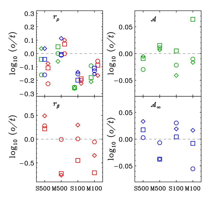
Since we need to fix the values of the haloes before stacking, cannot be a free parameter of the MAMPOSSt analysis. Moreover, in an effort to mimick the observational procedure, we estimate the individual values of the 11 haloes also before stacking, and then we take the biweight average of these values as representative of the of the stack. In the real world, this is done because individual haloes often suffer from different spectroscopic incompleteness levels. More precisely, we take the estimates obtained in the EVir case (see Sect. 3.4). The remaining two parameters, and the anisotropy parameter are estimated via the MAMPOSSt analysis. Results for the six stacked haloes are listed in Table 5 and displayed in Fig. 8. We use the gapper estimate of dispersion (Wainer & Thissen, 1976, see Beers et al., 1990) given our small sample ().

In Fig. 9, we show 1-, 2-, and 3- contours in the plane (for the T anisotropy model). In this figure, we indicate with a cross the expected solution for the stacked haloes. This is the biweight-average (with its error) of the true and values of the 11 individual haloes from which the stacked haloes are constructed. These values are also listed in the last line of Table 1. The average values of and are identical, in substantial agreement with what was found by MBM10. Note also that the average value of corresponds to , meaning that the average ML and T anisotropy models are the same.
Fig. 9 shows that the expected solution for the stack sample is always within the 1- contour of the MAMPOSSt result for the T model. While not shown, this is also the case for the Cst model, but not for the ML model, where remains essentially unconstrained, as was the case for the individual haloes. The estimates of the parameter do not depend on the assumed anisotropy model. They are biased low for the stacks built from the 100-particle samples, even if not significantly so (see Fig. 9). Interestingly, while the bias is stronger for the 100-particle stack than for the 500-particle one, the dispersion of the recovered values appears to be lower. The dispersion is instead higher, as expected, for the anisotropy parameters, except for where the dispersion is comparable for the 500-particle and the 100-particle stacks. However, with only three results per anisotropy model for each Stack sample, these differences in bias and dispersions do not appear to be statistically significant.
In Table 5, we also list the biweight average values of the 11 individual haloes along each projection, obtained in the EVir case (see Sect. 3.4), and these values are also plotted in Fig. 8 (labelled ‘M’) together with the best-fit solutions for the stacked haloes (labelled ‘S’). Comparing the best-fit values of and the anisotropy parameters obtained from the stacked haloes with those found from the mean of the individual 11 haloes (along the same projection), it is difficult to decide whether it is better to run MAMPOSSt on the stacked halo or to adopt means of the individual MAMPOSSt estimates. A close inspection of Table 5 and Fig, 8 indicates that, for , stacks are more accurate for estimating and , while means of individual MAMPOSSt estimates appear more accurate for estimating and . But the statistics are poor. In the real observational situation, it therefore seems advisable to consider both the average of the results of the individual haloes and the result obtained for the stacked sample.
3.6 A large halo
| Projection | anisotropy | |||||
|---|---|---|---|---|---|---|
| 4529 | Cst | 1.538 | 0.499 | 0.262 | 1.053 | |
| 4520 | Cst | 1.747 | 0.369 | 0.352 | 1.122 | |
| 4662 | Cst | 1.642 | 0.318 | 0.197 | 1.252 | |
| bias | –0.005 | –0.024 | –0.190 | –0.096 | ||
| inefficiency | 0.033 | 0.116 | 0.149 | 0.044 | ||
| 4529 | ML | 1.505 | 0.499 | 0.308 | 0.568 | |
| 4520 | ML | 1.711 | 0.370 | 0.352 | 0.638 | |
| 4662 | ML | 1.621 | 0.318 | 0.190 | 0.301 | |
| bias | –0.013 | –0.023 | –0.142 | 1.080 | ||
| inefficiency | 0.033 | 0.115 | 0.158 | 0.192 | ||
| 4529 | T | 1.454 | 0.502 | 0.447 | 2.289 | |
| 4520 | T | 1.700 | 0.371 | 0.425 | 1.666 | |
| 4662 | T | 1.623 | 0.320 | 0.236 | 1.705 | |
| bias | –0.017 | –0.021 | 0.030 | –0.116 | ||
| inefficiency | 0.040 | 0.115 | 0.164 | 0.082 | ||
| 489 | Cst | 1.616 | 0.492 | 0.336 | 0.887 | |
| 460 | Cst | 1.773 | 0.398 | 0.340 | 1.156 | |
| 476 | Cst | 1.688 | 0.260 | 0.187 | 1.188 | |
| bias | 0.008 | –0.036 | –0.081 | –0.084 | ||
| inefficiency | 0.024 | 0.164 | 0.154 | 0.075 | ||
| 489 | ML | 1.554 | 0.494 | 0.483 | 0.764 | |
| 460 | ML | 1.739 | 0.399 | 0.335 | 0.562 | |
| 476 | ML | 1.672 | 0.261 | 0.195 | 0.310 | |
| bias | –0.001 | –0.034 | –0.107 | 1.015 | ||
| inefficiency | 0.029 | 0.164 | 0.232 | 0.231 | ||
| 489 | T | 1.454 | 0.496 | 0.676 | 3.454 | |
| 460 | T | 1.724 | 0.401 | 0.412 | 1.735 | |
| 476 | T | 1.677 | 0.261 | 0.247 | 1.829 | |
| bias | 0.010 | –0.033 | 0.003 | –0.092 | ||
| inefficiency | 0.044 | 0.165 | 0.258 | 0.177 | ||
Notes: The results are for Case Gen. Col. 1: viewing axis; col. 2: number of particles after interloper removal with the Clean method; col. 3: anisotropy model; col. 4: virial radius; col. 5: tracer scale radius; col. 6: DM scale radius; col. 7: anisotropy parameter ( for Cst, for ML and for T); The biases and inefficiencies are respectively computed from biweight means and gapper standard deviations of the 3 values (following Beers et al., 1990).
It is interesting to consider whether we can achieve the same accuracy using a single halo, but with a total number of tracer particles similar to that of the stack. We extract particles within for the more massive halo in our sample, 5726, remove interlopers with the Clean method, and run MAMPOSSt for the general case, adopting the NFW mass density and different anisotropy models.
Table 6 compares the results for the 3 cones of 500 particles (counted before interloper removal) and the 3 with 5000 particles. We use again the gapper dispersion, given our small sample (). As expected, the biases and inefficiencies are generally reduced when selecting all (5000) particles instead of randomly selecting 500. For the T anisotropy model, the inefficiencies in are reduced by 0.1 dex for and anisotropy, 0.15 dex for , but virtually unchanged for . Surprisingly, for Cst and ML anisotropy, is reached with worse inefficiency with the full 5000-particle sample in comparison with the 500-particle one.
However, one should not over-interpret these comparisons. Indeed, our Monte-Carlo tests on 10 000 random samples of 3 objects arising from a Gaussian distribution indicate that while the gapper standard deviation is unbiased even for as few as 3 objects, it has an inefficiency of 0.53 times its true value for . In other words, an inefficiency of of 0.1 would have roughly 0.05 accuracy. Therefore, any improvement or worsening of inefficiency in of less than a factor of 2 is clearly not statistically significant. Nevertheless, the fact that most inefficiencies are reduced when increasing the sample size from 500 to 5000 is much more significant, and is indeed what is qualitatively expected. However, the expected quantitative improvement of does not appear to be attained for the inefficiency of .
The bias and inefficiencies for the 5000-particle sample are typically higher for the single halo than for the particle stack (with just 10% more particles, although the extraction there was for case EVir instead of Gen). But again, the inefficiencies are within a factor 2, so these changes are individually not statistically significant. But the combination of all of them appears to be statistically significant.
The worse inefficiencies for the large halo in comparison with the stacked halo of similar number of tracers can be due to either our assumption of Gaussian velocity distributions (see Sect. 2.2) or to the triaxiality of the halo velocity ellipsoids. The velocity distribution of the stack halo approaches a Gaussian by the central limit theorem, so our Gaussian assumption is better verified in a stack sample than in individual haloes. As a matter of fact, a number of studies have shown the 3D velocity distributions of individual haloes to deviate from Gaussianity (Wojtak et al., 2005; Hansen et al., 2006). But perhaps the dominant effect is that of triaxiality. As discussed at the end of Sect. 3.4, the results obtained by MAMPOSSt for are influenced by the choice of the projection axis, and in the present case, the values obtained for 5726 along the , , and projections when using 5000 particles, are ordered in the same way as those obtained when using 500 particles.
4 Conclusions and Discussion
We have presented the formalism for a new method, called MAMPOSSt, for the determination of the mass and anisotropy profiles of spherical systems, assumed to be in dynamical equilibrium, in particular, as stationary systems with no streaming motions. In MAMPOSSt, the distribution of tracers in projected phase space are fit by the predicted distribution arising from assumed 3D radial profiles of the tracer density, total mass, and velocity anisotropy, as well from an assumed family of shapes for the radial and tangential components of the 3D velocity distribution.
MAMPOSSt has several important advantages over other methods for mass/anisotropy modeling:
- 1).
MAMPOSSt does not involve binning the data, hence its results are independent of the choice of such radial bins, in contrast with methods based upon velocity moments, including anisotropy and mass inversions;
- 2).
MAMPOSSt does not involve interpolations and extrapolations of binned radial profiles of the observables, again in contrast with anisotropy and mass inversions;
- 3).
MAMPOSSt does not require differentiation of the observed projected pressure, , once more in contrast with anisotropy and mass inversions;
- 4).
MAMPOSSt extracts accurate constraints on the velocity anisotropy, in contrast with methods that assume Gaussian LOS velocity distributions;
- 5).
MAMPOSSt is very fast, as it involves a single integral (for popular profiles). Indeed, the calculations for the best fit parameters and their marginal and correlated distributions through MCMC for a 500-tracer system (as displayed in Fig. 2) require roughly 4 minutes of CPU time on a standard desktop personal computer. By contrast, distribution function methods involve triple integrals, and therefore take typically 1000 times longer to run, i.e. a few days for 500-tracer systems. Orbit modeling techniques are even slower and cannot properly probe parameter space.
In this work, we have extensively tested MAMPOSSt, for the case of Gaussian 3D velocity distributions, on a set of 11 cluster-mass haloes extracted from cosmological simulations. The results of these tests indicate that, for systems with 500 velocities, MAMPOSSt provides essentially unbiased estimates of the relevant mass and velocity anisotropy profile parameters, with inefficiencies of 10% for the virial radius, 20% for the constant or outer velocity anisotropy, 27% for the tracer scale radius, but as high as 48% for the scale radius of the DM. However, MAMPOSSt seems unable to set constraints on the radius of transition of a gently rising anisotropy model such as ML.
We have noted that the results of MAMPOSSt are similar when we inserted the virial radius among the parameters to be jointly fit or when we derived the virial radius using the new interloper removal scheme that we presented in Appendix B. We found that this interloper-removal algorithm performs as well or better than other methods.

As shown in Fig. 10, the errors on from MAMPOSSt are highly correlated with those obtained from the Clean procedure. Hence, the new interloper removal scheme produces extremely fast estimates of the virial radius, based on the LOS velocity dispersion, that are very close to those obtained with the full MAMPOSSt procedure.
The correlation highlighted in Fig. 10 suggests that the quality of MAMPOSSt estimates is limited by the accuracy of the interloper removal. However, we also saw (Fig. 7) that the error on is correlated with the ratio of velocity dispersions within the true virial sphere, measured along the projection axis over that measured globally. This second correlation indicates that our capability of recovering the true values of is limited by the effects of triaxiality, i.e. by the fact that we only observe one component of the 3-dimensional velocity distribution. The effect of triaxiality may be even more important than the uncertainties in the interloper cleaning process.
Our additional tests lead to the following conclusions:
- 1).
Best results are obtained setting all 4 parameters free and using the T anisotropy model.
- 2).
Setting the virial radius to the true value (e.g. measured through other techniques, such as X-rays or lensing) leads to worse results on the other parameters than when the virial radius is an additional free parameter. We argue that this is caused by the triaxiality of the haloes (Fig. 7).
- 3).
MAMPOSSt works surprisingly well with samples of 100 tracers instead of 500, only somewhat better with samples of 5000 tracers, even better with stacked haloes of tracers, similar to the mean of these individual tracers, but not well as expected from arguments.
- 4).
MAMPOSSt is not very sensitive to the chosen aperture, when this is to within 35% of the true value of .
| Method | Reference | Particles | |||||||||||
|---|---|---|---|---|---|---|---|---|---|---|---|---|---|
| bias | ineff. | bias | ineff. | bias | ineff. | bias | ineff. | ||||||
| Dispersion-kurtosis | Sanchis et al. (2004) | 400 | –0.023 | 0.033 | 0.080 | 0.240 | –0.040 | 0.110 | — | — | |||
| MAMPOSSt =cst | this article | 400 | 0.004 | 0.040 | –0.030 | 0.289 | –0.010 | 0.069 | — | — | |||
| Distribution function | Wojtak et al. (2009) | 300 | –0.026 | 0.048 | 0.017 | 0.169 | — | — | –0.002 | 0.212 | |||
| MAMPOSSt -T | this article | 300 | –0.003 | 0.044 | 0.017 | 0.198 | — | — | –0.016 | 0.116 | |||
Notes: The biases and inefficiencies on virial masses for the dispersion-kurtosis and distribution function methods were divided by 3 to convert to biases and inefficiencies for virial radii. All analyses are for case TLM, and for MAMPOSSt the Clean interloper removal scheme is used. Dispersion-kurtosis for the DM scale radius were taken from the analogous values that Sanchis et al. (2004) obtained for the concentration parameter (basically assuming that in comparison, the errors on the virial radius are small). For the distribution function method, values of for the outer anisotropy were measured at roughly the virial radius, while the MAMPOSSt comparison (last row) is for the T anisotropy model (eq. [38]). The biases and inefficiencies are estimated with the biweight mean and dispersion, except for the dispersion-kurtosis method, where they are taken from the 2nd line of Table 3 of Sanchis et al.. Values where MAMPOSSt is better are highlighted in bold.
Table 7 compares the accuracy of MAMPOSSt with that of the dispersion-kurtosis method of Łokas (2002, tested by Sanchis, Łokas, & Mamon, 2004) and the DF method of Wojtak et al. (2009). In comparison with the dispersion-kurtosis method, MAMPOSSt does slightly less well on the inefficiencies of the virial radius and worse on that of the DM scale radius (but better on the biases of both radii), but MAMPOSSt performs better for the constant anisotropy (both bias and inefficiency). Moreover, MAMPOSSt has the advantage of being flexible enough to infer the outer anisotropy, while the dispersion-kurtosis method of Łokas (2002) is limited to constant anisotropy (but this limitation to the dispersion-kurtosis method has been recently lifted by Richardson & Fairbairn, 2012). Comparing with the much slower DF method, MAMPOSSt does somewhat worse on the inefficiency on the scale radius, with the same bias, yet MAMPOSSt is respectively slightly (not significantly) and much better on the inefficiencies on the virial radius and outer anisotropy, with less bias on the former. Note, however, that we forced here the inner velocities to be isotropic, while these were free parameters in the DF method and that the DF method computes the outer anisotropies at instead of the asymptotic value. Nevertheless, we found (Table 4) that MAMPOSSt always performs as well or better when all parameters are set free, and we would expect the same for the DF method. Moreover, we see no reason why the inefficiency of the anisotropy measured near the virial radius should be worse than that of its asymptotic value.
Despite the very good results of our tests, it must be noted that although the Gaussian MAMPOSSt recovers the 2nd velocity moment (eq. [30]) , it does not recover the fourth moment. Indeed, taking the fourth moment of the velocity distribution of equation (28) leads to
| (40) | |||||
where the second equality of equation (40) is obtained after reversing the order of integration, while the final equality uses equation (26). Equation (40) then gives the LOS velocity kurtosis excess
| (41) |
Unfortunately, the expression for the fourth velocity moment in equation (40) differs from the expression found by Łokas (2002) from the 4th order Jeans equation in the case of . At large projected radius (), estimated by equations (40) and (41) turns out to be nearly independent of . This shows the limit of the Gaussian approximation for the 3D velocity distribution.
Nevertheless, despite the poor adequacy of the Gaussian approximation, which does not produce the correct LOS kurtosis profiles, MAMPOSSt with Gaussian velocities performs quite well according to our numerous tests. We are therefore confident that the method is mature for being used on real data-sets. And we are preparing analyses on several scales: dwarf spheroidal galaxies, giant ellipticals (traced by planetary nebulae), groups and clusters of galaxies. We also plan to test MAMPOSSt on elliptical galaxies formed in dissipative mergers.
One should note that in CDM haloes, the 3D velocity distribution, measured in shells, is not Gaussian (Wojtak et al., 2005), but resembles the -Gaussian distribution, which generalizes the Gaussian distribution in the same way as Tsallis (1988) entropy generalizes Boltzmann-Gibbs entropy. The -Gaussian (often called Tsallis) fits well a host of velocity distributions found in single-component dissipationless self-gravitating systems, with an index that varies linearly with the slope of the density profile (Hansen et al., 2006). We are thus preparing a generalization of MAMPOSSt to the Tsallis distribution of 3D velocities (appropriately combining radial and tangential terms), and expect this to perform even better than the MAMPOSSt-Gaussian algorithm.
Acknowledgements
We gratefully acknowledge the anonymous referee for constructive comments that strengthened our work, and Leandro José Beraldo e Silva for his critical reading of the manuscript. We thank Giuseppe Murante for providing us with the cosmological simulation and Anthony Lewis for developing and maintaining the CosmoMC MCMC code. Thanks also to Michael Powell for making his NEWUOA minimization code public, and Radek Wojtak for supplying his test output in digital form.
References
- Ascasibar & Gottlöber (2008) Ascasibar Y., Gottlöber S., 2008, MNRAS, 386, 2022
- Bartelmann (1996) Bartelmann M., 1996, A&A, 313, 697
- Battaglia et al. (2008) Battaglia G., Helmi A., Tolstoy E., Irwin M., Hill V., Jablonka P., 2008, ApJ, 681, L13
- Beers et al. (1990) Beers T. C., Flynn K., Gebhardt K., 1990, AJ, 100, 32
- Binney & Mamon (1982) Binney J., Mamon G. A., 1982, MNRAS, 200, 361
- Biviano & Girardi (2003) Biviano A., Girardi M., 2003, ApJ, 585, 205
- Biviano et al. (2006) Biviano A., Murante G., Borgani S., Diaferio A., Dolag K., Girardi M., 2006, A&A, 456, 23
- Biviano & Poggianti (2009) Biviano A., Poggianti B. M., 2009, A&A, 501, 419
- Borgani et al. (2004) Borgani S. et al., 2004, MNRAS, 348, 1078
- Burkert (1995) Burkert A., 1995, ApJ, 447, L25
- Carlberg et al. (1997) Carlberg R. G., Yee H. K. C., Ellingson E., 1997, ApJ, 478, 462
- Cuesta et al. (2008) Cuesta A. J., Prada F., Klypin A., Moles M., 2008, MNRAS, 389, 385
- Dejonghe (1989) Dejonghe H., 1989, ApJ, 343, 113
- Dejonghe & Merritt (1992) Dejonghe H., Merritt D., 1992, ApJ, 391, 531
- den Hartog & Katgert (1996) den Hartog R., Katgert P., 1996, MNRAS, 279, 349
- Diemand et al. (2004) Diemand J., Moore B., Stadel J., 2004, MNRAS, 352, 535
- Einasto (1965) Einasto J., 1965, Trudy Inst. Astroz. Alma-Ata, 51, 87
- Gerhard et al. (1998) Gerhard O., Jeske G., Saglia R. P., Bender R., 1998, MNRAS, 295, 197
- Gerhard (1993) Gerhard O. E., 1993, MNRAS, 265, 213
- Girardi et al. (1993) Girardi M., Biviano A., Giuricin G., Mardirossian F., Mezzetti M., 1993, ApJ, 404, 38
- Gnedin et al. (2004) Gnedin O. Y., Kravtsov A. V., Klypin A. A., Nagai D., 2004, ApJ, 616, 16
- Haardt & Madau (1996) Haardt F., Madau P., 1996, ApJ, 461, 20
- Hansen et al. (2010) Hansen S. H., Juncher D., Sparre M., 2010, ApJ, 718, L68
- Hansen & Moore (2006) Hansen S. H., Moore B., 2006, New Astronomy, 11, 333
- Hansen et al. (2006) Hansen S. H., Moore B., Zemp M., Stadel J., 2006, JCAP, 1, 14
- Hernquist (1990) Hernquist L., 1990, ApJ, 356, 359
- Katgert et al. (2004) Katgert P., Biviano A., Mazure A., 2004, ApJ, 600, 657
- Kronawitter et al. (2000) Kronawitter A., Saglia R. P., Gerhard O., Bender R., 2000, A&AS, 144, 53
- Lemze et al. (2012) Lemze D. et al., 2012, ApJ, 752, 141
- Lewis & Bridle (2002) Lewis A., Bridle S., 2002, Phys. Rev. D, 66, 103511
- Łokas (2002) Łokas E. L., 2002, MNRAS, 333, 697
- Łokas & Mamon (2001) Łokas E. L., Mamon G. A., 2001, MNRAS, 321, 155
- Łokas & Mamon (2003) Łokas E. L., Mamon G. A., 2003, MNRAS, 343, 401
- Ludlow et al. (2009) Ludlow A. D., Navarro J. F., Springel V., Jenkins A., Frenk C. S., Helmi A., 2009, ApJ, 692, 931
- Macciò et al. (2008) Macciò A. V., Dutton A. A., van den Bosch F. C., 2008, MNRAS, 391, 1940
- Mamon et al. (2010) Mamon G. A., Biviano A., Murante G., 2010, A&A, 520, A30
- Mamon & Boué (2010) Mamon G. A., Boué G., 2010, MNRAS, 401, 2433
- Mamon & Łokas (2005) Mamon G. A., Łokas E. L., 2005, MNRAS, 363, 705
- Mauduit & Mamon (2007) Mauduit J.-C., Mamon G. A., 2007, A&A, 475, 169
- Merritt (1985) Merritt D., 1985, MNRAS, 214, 25P
- Merritt (1987) Merritt D., 1987, ApJ, 313, 121
- Merritt & Saha (1993) Merritt D., Saha P., 1993, ApJ, 409, 75
- Navarro et al. (1996) Navarro J. F., Frenk C. S., White S. D. M., 1996, ApJ, 462, 563
- Navarro et al. (2004) Navarro J. F. et al., 2004, MNRAS, 349, 1039
- Newman et al. (2009) Newman A. B., Treu T., Ellis R. S., Sand D. J., Richard J., Marshall P. J., Capak P., Miyazaki S., 2009, ApJ, 706, 1078
- Osipkov (1979) Osipkov L. P., 1979, Soviet Astronomy Letters, 5, 42
- Powell (2006) Powell M. J. D., 2006, in Nonconvex Optimization and Its Applications, Di Pillo G., Roma M., eds., Vol. 83, Spinger, pp. 255–297
- Richardson & Fairbairn (2012) Richardson T., Fairbairn M., 2012, MNRAS, submitted, arXiv:1207.1709
- Richstone & Tremaine (1984) Richstone D. O., Tremaine S., 1984, ApJ, 286, 27
- Sanchis et al. (2004) Sanchis T., Łokas E. L., Mamon G. A., 2004, MNRAS, 347, 1198
- Schwarzschild (1979) Schwarzschild M., 1979, ApJ, 232, 236
- Sparre & Hansen (2012) Sparre M., Hansen S. H., 2012, JCAP, 10, 49
- Springel & Hernquist (2003) Springel V., Hernquist L., 2003, MNRAS, 339, 289
- Springel et al. (2005) Springel V. et al., 2005, Nature, 435, 629
- Strigari et al. (2008) Strigari L. E., Bullock J. S., Kaplinghat M., Simon J. D., Geha M., Willman B., Walker M. G., 2008, Nature, 454, 1096
- Syer & Tremaine (1996) Syer D., Tremaine S., 1996, MNRAS, 282, 223
- Tiret et al. (2007) Tiret O., Combes F., Angus G. W., Famaey B., Zhao H. S., 2007, A&A, 476, L1
- Tsallis (1988) Tsallis C., 1988, Journal of Statistical Physics, 52, 479
- van der Marel (1994) van der Marel R. P., 1994, MNRAS, 270, 271
- van der Marel & Franx (1993) van der Marel R. P., Franx M., 1993, ApJ, 407, 525
- Wainer & Thissen (1976) Wainer H., Thissen D., 1976, Psychometrica, 41, 9
- Walker et al. (2009) Walker M. G., Mateo M., Olszewski E. W., Peñarrubia J., Evans N. W., Gilmore G., 2009, ApJ, 704, 1274
- Wojtak et al. (2005) Wojtak R., Łokas E. L., Gottlöber S., Mamon G. A., 2005, MNRAS, 361, L1
- Wojtak et al. (2009) Wojtak R., Łokas E. L., Mamon G. A., Gottlöber S., 2009, MNRAS, 399, 812
- Wojtak et al. (2008) Wojtak R., Łokas E. L., Mamon G. A., Gottlöber S., Klypin A., Hoffman Y., 2008, MNRAS, 388, 815
- Wojtak et al. (2007) Wojtak R., Łokas E. L., Mamon G. A., Gottlöber S., Prada F., Moles M., 2007, A&A, 466, 437
- Wojtak & Mamon (2013) Wojtak R., Mamon G. A., 2013, MNRAS, 428, 2407
- Wolf et al. (2010) Wolf J., Martinez G. D., Bullock J. S., Kaplinghat M., Geha M., Muñoz R. R., Simon J. D., Avedo F. F., 2010, MNRAS, 406, 1220
- Zabludoff et al. (1993) Zabludoff A. I., Franx M., Geller M. J., 1993, ApJ, 419, 47
- Zhao (1996) Zhao H., 1996, MNRAS, 278, 488
Appendix A Kernels for determining the radial velocity dispersion profile from the Jeans equation
The radial squared velocity dispersion profile of equation (9) can be written (van der Marel, 1994; Mamon & Łokas, 2005)
| (42) |
where is the solution to , i.e.
| (43) |
For simple anisotropy models (not all are used in this work),
| (44) |
where is the Osipkov-Merritt anisotropy model (Osipkov, 1979; Merritt, 1985), is the Mamon-Łokas anisotropy model (Mamon & Łokas, 2005), is a generalization of the Mamon-Łokas model by Tiret et al. (2007), is another model that fits well the anisotropy of CDM haloes with (Diemand, Moore, & Stadel, 2004), while the last two rows describe the anisotropy that varies linearly with the slope of the density profile (Hansen & Moore, 2006), since the kernel depends on the precise form of the density profile. The first of these last two rows gives the kernel for Zhao’s (1996) general density profile
| (45) |
where and are the inner and outer logarithmic slopes of the density profile (i.e. and for the NFW model), and is the radius of slope , while is the radius of slope . The last row is for the Einasto (1965) density profile
| (46) |
which, for , is an excellent fit to the density profiles of simulated CDM haloes (Navarro et al., 2004), while is an excellent fit to the dark matter density profiles of haloes in hydrodynamical CDM cosmological simulations (MBM10).
Appendix B Interloper removal
This appendix describes how we remove obvious (high absolute line-of-sight velocity) interlopers.
We analyze the DM particles in the output of the hydrodynamical cosmological simulation of Borgani et al. (2004), to which we added the Hubble flow, placed an observer at from each of the 105 most massive haloes (including the most irregular ones), in each of the three cartesian directions. We limited these haloes to projected radii within from the barycentre of the Friends-of-Friends halo identified in real space, where , 1 or 1.4, and within line-of-sight velocities within 4 times the true circular velocity at the from the true velocity centre (see MBM10 for details). The choice for the three values of is to consider cases where the observers guess incorrectly the virial radius when they select their galaxies. We only used the 274 haloes out of 315 that had at least 500 particles with .66 6 We used an output of the simulation with 1 particle out of 55 chosen at random.
We chose particles at random in the projected phase space, so that we ended up with approximately particles with , i.e. for or and 620 for and 1.4, respectively, where we assumed a concentration , typical of the haloes of our simulation (MBM10). The projected mass of the NFW model is , where is the radius where the logarithmic of the density profile is and the dimensionless projected mass is (Łokas & Mamon, 2001, first derived by Bartelmann, 1996 in a slightly longer and more computer intensive form)
| (47) |
Our algorithm for interloper rejection, which is Bayesian as it assumes what we know about CDM haloes, namely that they approximately follow NFW density profiles with increasingly radial orbits, goes as follows.
- i).
On first pass, we apply the gapper (or weighted gap) technique in order to split multimodal distributions of the distribution of velocities , and identify the peak in velocity space closest to the input mean velocity of the halo, which we assume to know. After sorting the velocity offsets, we compute weighted gaps
(48) for . We then check if the largest value of the dimensionless gap is greater than some threshold, commonly called (MidMean is the arithmetic mean within the quartiles of the distribution). Among all the subsamples separated by a dimensionless gap , we keep only that one closest to the input mean velocity of the halo. The gapper technique (Wainer & Thissen, 1976) was first used in astronomy in the ROSTAT package77 7 By T. Beers, see http://www.pa.msu.edu/ ftp/pub/beers/posts/rostat/, which recommends and was first applied to detect multimodal populations in clusters of galaxies by Girardi et al. (1993), who used . This is also the value we use here.
- ii).
Using the velocities of the particles in the subsample identified with the gapper technique, we compute, in a first step, the global velocity dispersion of our selected particles, using the robust median absolute deviation (MAD), with where (e.g. Beers et al., 1990).
- iii).
We then estimate the virial velocity , from the relation
(49) (50) where , , and are the dimensionless radial profiles of density, mass and projected mass, respectively. Equation (49) was derived using the relation (Mamon & Łokas, 2005)
(51) with a kernel that has been derived by Mamon & Łokas for simple anisotropy profiles. In equation (50), we assume ML anisotropy (eq. [37]) with as found in a cosmological simulation by MBM10. We then derive from equation (50). We adopt the NFW model, with dimensionless mass density , dimensionless mass and dimensionless projected mass density given in equation (47). With the Mamon & Łokas anisotropy profile, and , the aperture velocity dispersion is well approximated (to better than 0.1% relative accuracy in the range ) by
(52) where , , , and . The ratio reaches a minimum of 0.65 at , with values of 0.69 at and 10. Had we assumed isotropy instead, would have been 3% lower (Mauduit & Mamon, 2007). In this first pass, we assume , while in subsequent passes we use the relation obtained in CDM haloes by Macciò et al. (2008): .
- iv).
We deduce an estimated virial radius , with overdensity . We use to conform with the positional units of the simulation (and which we had thus assumed for the Hubble flow).
- v).
Next, we compute LOS velocity dispersion predicted for the NFW model with anisotropy profile of equation (37) at the projected radius of every particle. For this, we use the approximation
(53) with the coefficients given in Table 2 (for the NFW column) of MBM10 and
(54) (e.g., eq. [22] of MBM10).
- vi).
We filter the particles to have velocities within times the local LOS velocity dispersion from the global median velocity. We adopt , which best preserves the LOS velocity dispersion profile (MBM10).
- vii).
We compute the global velocity dispersion of our velocity-filtered sample, this time using the standard unbiased standard deviation.
- viii).
We iterate, checking (except after the first pass) that the number of particles has changed or that had changed by more than 0.1%, by returning to step iii).
- ix).
On convergence, we select all particles within from the median (except for those filtered out by the gapper technique).
The novelty of this algorithm is that 1) it uses a guess of the (local) LOS velocity dispersion, and 2) it uses a cut at instead of 3 to optimally recover (MBM10).