Separated Structure Functions for Exclusive $K^{+}\Lambda$ and $K^{+}\Sigma^{0}$ Electroproduction at 5.5 GeV with CLAS

Hadrodynamic models provide a description of the reaction based on contributions from tree-level Born and extended Born terms in the $s$, $t$, and $u$ reaction channels (see Fig. 1). The Born diagrams include the exchange of the proton, kaon, and ground-state hyperons, while the extended Born diagrams include the exchange of the associated excited states. This description of the interaction, which involves only first-order terms, is sensible as the incident and outgoing electrons interact rather weakly with the hadrons. A complete description of the physics processes requires taking into account all possible channels that could couple to the initial and final states, but the advantages of the tree-level approach are to limit complexity and to identify the dominant trends. The drawback in this class of models is that very different conclusions about the strengths of the contributing diagrams may be reached depending on which set of resonances a given model includes.

Maxwell et al. [27, 33, 34] have developed a tree-level effective Lagrangian model (referred to as MX) for $\gamma^{(*)}p\to K^{+}\Lambda$ that incorporates the well-established $s$-channel resonances up to 2.2 GeV with spins up to 5/2. The model also includes four $\Lambda$ $u$-channel states, $\Lambda(1405)1/2^{-}$, $\Lambda(1670)1/2^{-}$, $\Lambda(1820)5/2^{+}$, $\Lambda(1890)3/2^{+}$, four $\Sigma$ $u$-channel states, $\Sigma(1385)3/2^{+}$, $\Sigma(1775)5/2^{-}$, $\Sigma(1915)5/2^{+}$, $\Sigma(1940)3/2^{-}$, and the $K^{*}(892)$ and $K_{1}(1270)$ $t$-channel resonances.

The model was initially developed and fit to the available $\gamma p$ photoproduction data up to $W$=2.3 GeV [34]. The most recent published version of the model [27] included fits to the available $K^{+}\Lambda$ separated structure function data from CLAS [16]. An extension of this model that also includes fits to the available CLAS $K^{+}\Lambda$ $\sigma_{LT^{\prime}}$ data has been made available for this work as well. Overall the fits yield reasonable representations of both the photo- and electroproduction data. However, when compared to the results of a fit to the photoproduction data alone, the combined $\gamma p$ and $\gamma^{*}p$ fit yields significantly different coupling parameters for an equally good overall fit to the data. This indicates that the photoproduction data alone are not adequate to uniquely constrain effective Lagrangian models of electromagnetic strangeness production.

Our $KY$ electroproduction data are also compared to the Regge model from Guidal, Laget, and Vanderhaeghen [35] (referred to as GLV). This calculation includes no baryon resonance terms at all. Instead, it is based only on gauge-invariant $t$-channel $K$ and $K^{*}$ Regge-trajectory exchange. It therefore provides a complementary basis for studying the underlying dynamics of strangeness production. It is important to note that the Regge approach has far fewer parameters compared to the hadrodynamic models. These include the $K$ and $K^{*}$ form factors and the coupling constants $g_{KYN}$ and $g_{K^{*}YN}$.

The GLV model was fit to higher-energy photoproduction data where there is little doubt of the dominance of kaon exchanges, and extrapolated down to JLab energies. An important feature of this model is the way gauge invariance is achieved for the kaonic $t$-channel exchanges by Reggeizing the $s$-channel nucleon pole contribution in the same manner as the $t$-channel diagrams. No counter terms need to be introduced to restore gauge invariance as is done in the hadrodynamic approach.

The GLV Regge model reasonably accounts for the strength in the CLAS $K^{+}\Lambda$ differential cross sections and separated structure functions [16]. Although the reasonable performance of a pure Regge description in this channel suggests a $t$-channel dominated process, there are obvious discrepancies between the Regge predictions and the data, indicative of $s$-channel strength. In the $K^{+}\Sigma^{0}$ channel, the same Regge description significantly underpredicts the differential cross sections and separated structure functions [16]. The fact that the Regge model fares poorly when compared to the $K^{+}\Sigma^{0}$ data is indicative that this process has a much larger $s$-channel content compared to $K^{+}\Lambda$ production.

The final model included in this work was developed by the Ghent group [26], and is based on a tree-level effective field model for $K^{+}\Lambda$ and $K^{+}\Sigma^{0}$ photoproduction from the proton. It differs from traditional isobar approaches in its description of the non-resonant diagrams, which involve the exchange of $K$ and $K^{*}$ Regge trajectories. A selection of $s$-channel resonances is then added to this background. This “Regge plus resonance” model (referred to as RPR) has the advantage that the background diagrams contain only a few parameters that are tightly constrained by high-energy data. Furthermore, the use of Regge propagators eliminates the need to introduce strong form factors in the background terms, thus avoiding the gauge-invariance issues associated with traditional effective Lagrangian models.

In addition to the kaonic trajectories to model the $t$-channel background, the RPR model includes the same $s$-channel resonances as for the MX model below 2 GeV. The model does include several missing $N^{*}$ states at 1.9 GeV, $N(1900)3/2^{-}$, $N(1900)3/2^{-}$, and $N(1900)1/2^{+}$. The separated structure functions [16, 17] and beam-recoil transferred polarization data from CLAS [15] were compared to model variants with either a $N(1900)3/2^{-}$ or a $N(1900)1/2^{+}$ state at 1.9 GeV. Only the $N(1900)3/2^{-}$ state assumption could be reconciled with the data, whereas the $N(1900)1/2^{+}$ option could clearly be rejected. In the $K^{+}\Sigma^{0}$ channel, four $\Delta^{*}$ states, $\Delta(1700)3/2^{-}$, $\Delta(1900)1/2^{-}$, $\Delta(1910)1/2^{+}$, and $\Delta(1920)3/2^{+}$, have been included.

In a new version of the RPR model (referred to as RPR-2011) [36], several changes relative to the previous model version (referred to as RPR-2007) [26] are noteworthy. The main difference is the implementation of an unbiased model selection methodology based on Bayesian inference. This inference is used as a quantitative measure of whether the inclusion of a given set of $N^{*}$ states is justified by the data. Additionally, in this version of the model, the exchange of spin-3/2 resonances is described within a consistent interaction theory and the model has been extended to include the exchange of spin 5/2 resonances.

The Regge background amplitude of RPR-2007 is constrained by spectra above the resonance region ($W>3$ GeV) at forward angles ($\cos\theta_{K}^{*}>0.35$). By extrapolating the resulting amplitude to smaller $W$, one gets a parameter free background for the resonance region. The $s$-channel resonances are coherently added to the background amplitude. RPR-2007 describes the data for forward-angle photo- and electroproduction of $K^{+}\Lambda$ and $K^{+}\Sigma^{0}$. The resonance parameters of the RPR-2007 model are constrained to the $\cos\theta_{K}^{*}>0.35$ data. The RPR-2011 model with the highest evidence has nine well-established $N^{*}$ states and the “missing” states at 1.9 GeV with quantum numbers $N(1900)3/2^{-}$ and $N(1900)1/2^{+}$, and has been fit to photoproduction data over the full $K^{+}$ center-of-mass (c.m.) angular range. Neither version of the model has been constrained by fits to any of the electroproduction data.

The statistical uncertainty on the cross section in each bin $i$ includes contributions from the statistical uncertainty on the hyperon yield and the acceptance function and is given by:

The $\gamma^{*}p\to K^{+}\Lambda$ and $\gamma^{*}p\to K^{+}\Sigma^{0}$ reaction channels were identified by detecting a scattered electron in coincidence with a $K^{+}$ and then using the missing mass technique to identify the hyperons. Event reconstruction required the identification of both a final state electron and $K^{+}$ candidate within the well-understood fiducial regions of the detector. Details on the algorithms employed to minimize the particle misidentification at this stage are included in Ref. [15]. Before computing the missing mass spectrum, vertex cuts were employed to ensure that the particles originated from the target. In addition, corrections to the electron and kaon momenta were devised to account for reconstruction inaccuracies that arose due to to relative misalignments of the drift chambers in the CLAS magnetic field, as well as from uncertainties in the magnetic field map employed during charged track reconstructions. These corrections were typically less than 1%.

The algorithm used for hadron identification relied on comparing the measured velocity $\beta=v/c$ for the track candidate to that expected for an assumed $\pi^{+}$, $K^{+}$, and $p$ track. The assumption that resulted in the minimum $\Delta\beta=\beta-\beta^{calc}_{\pi,K,p}$ was used to identify the species of the track. Fig. 3 shows $\Delta\beta$ versus momentum for the $K^{+}$ track assumption. For the data included here, the kaon momentum range was between 0.35 GeV (software cut) and $\approx$ 4.5 GeV (kinematic limit), with a typical flight path of 5.5 m. The measured mass resolution was primarily due to the reconstructed time-of-flight resolution, which was $\approx$100 ps ($\sigma$) on average; it also included contributions from the momentum and path length uncertainties of CLAS. Fig. 3 shows that unambiguous separation of $K^{+}$ tracks at the 2$\sigma$ level is possible up to about 2 GeV. For higher momenta, the background due to particle misidentification increases. Detailed background subtractions are necessary to determine the final event yields.

Fig. 4 shows the $e^{\prime}K^{+}$ missing mass ($MM(e^{\prime}K^{+})$) distribution for the final event sample after all cuts have been made. This distribution contains a background continuum beneath the hyperons that arises due to multi-particle final states where the candidate $K^{+}$ results from a misidentified pion or proton.

The data were binned in a four-dimensional space of the kinematic variables $Q^{2}$, $W$, $\cos\theta_{K}^{*}$, and $\Phi$. The bin definitions used in this analysis are listed in Table 1. Fig. 5 shows the kinematic extent of the data in terms of $Q^{2}$ versus $W$ and $\Phi$ versus $\cos\theta_{K}^{*}$. These plots are overlaid with a grid indicating the bins in this analysis. The bin widths in $W$ and $\Phi$ were chosen to be uniform. Note that the maximum $W$ bin at each $Q^{2}$ was limited to where the hyperon yield fits were not dominated by systematic uncertainties.

The three components of the $MM(e^{\prime}K^{+})$ spectra are the $K^{+}\Lambda$ events, the $K^{+}\Sigma^{0}$ events, and the particle misidentification background (dominated by pions misidentified as kaons). These individual contributions must be separated to extract the $K^{+}\Lambda$ and $K^{+}\Sigma^{0}$ differential cross sections in each analysis bin.

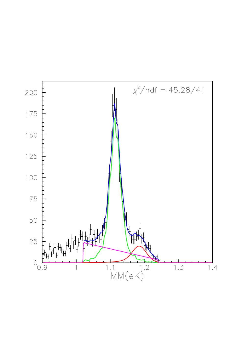
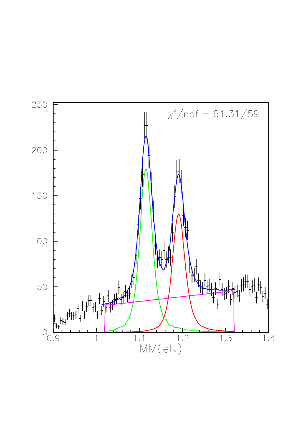
The hyperon templates were derived from a GEANT-based Monte Carlo that included radiative processes and was matched to the detector resolution (see Section IV.4.1). The background contributions for this fitting were studied with a number of different assumptions (see discussion in Section V). Ultimately, a linear form for the background was chosen. The template fits to the missing mass spectra were carried out using a maximum log likelihood method appropriate for the statistical samples of our data. Fig. 6 shows two sample fits to illustrate the typical fit quality to the data.

The final yields in each kinematic bin were determined by taking the number of counts determined from the fits that fell within a mass window around the $\Lambda$ (1.07 to 1.15 GeV) and $\Sigma^{0}$ (1.17 to 1.22 GeV) peaks. Hyperon events in the tails of the distributions that fell outside of the mass windows were accounted for by the acceptance and radiative corrections.

The number of $\Lambda$ and $\Sigma^{0}$ hyperons in both the $K^{+}\Lambda$ and $K^{+}\Sigma^{0}$ mass windows relative to the total number of counts in the mass windows was found to be independent of $Q^{2}$ and $\Phi$ in each bin of $W$ and $\cos\theta_{K}^{*}$. Thus the final yields in each bin were determined by scaling the raw yields in the $K^{+}\Lambda$ and $K^{+}\Sigma^{0}$ mass windows by a background factor determined from fits in each bin of $W$ and $\cos\theta_{K}^{*}$.

Radiative effects must be considered when determining the $\gamma^{*}p\to K^{+}Y$ cross sections. Radiative effects result in bin migration such that the measured $Q^{2}$ and $W$ are not the true $Q^{2}$ and $W$ to which the event should be properly associated.

For this analysis, two different approaches to determine these correction factors have been employed. The first uses the stand-alone program EXCLURAD [50] and the second uses the event generator GENEV [45] in combination with the CLAS Monte Carlo. The radiative correction factor that multiplies the measured bin-averaged differential cross section in each bin is defined as the ratio of the computed bin-averaged cross section with radiation off to that with radiation on. More details on each program are included below.

The goal of this analysis is to measure cross sections and separated structure functions for the $K^{+}Y$ final states at specific kinematic points. However, the analysis proceeds from using finite bins in the relevant kinematic quantities $Q^{2}$, $W$, $\cos\theta_{K}^{*}$, and $\Phi$ (see Section IV.2).

Studies of the bin-averaged kinematic quantities versus the geometric bin-centered values show that there is no need for bin-centering corrections in $W$ or $\cos\theta_{K}^{*}$. For this work the threshold $W$ bin for $K^{+}\Lambda$ is quoted at 1.630 GeV and for $K^{+}\Sigma^{0}$ at 1.695 GeV. To determine the bin-centering factor $BC_{i}$ for each bin, we have fit the measured structure functions $\sigma_{U}$ for each $W$ and $\cos\theta_{K}^{*}$ bin versus $Q^{2}$ for both the $K^{+}\Lambda$ and $K^{+}\Sigma^{0}$ final states. To bin center the data at specific $Q^{2}$ points, we have used the following dipole evolution factor:

The bin centering factors using this form were in the range from 0.95 to 1.05 across the full kinematic phase space.

In Fig. 10 we show a sample of the $\Phi$-dependent differential cross sections for the $K^{+}\Lambda$ final state at $W$=1.725 GeV for $Q^{2}$=1.8 GeV². The different shapes of the differential cross sections versus $\Phi$ in each of our bins in $Q^{2}$, $W$, and $\cos\theta_{K}^{*}$ reflect differences of the interference terms, $\sigma_{LT}$ and $\sigma_{TT}$, while the differences in scale reflect the differences in $\sigma_{U}$.

The extraction of $\sigma_{LT^{\prime}}$ in each bin of $Q^{2}$, $W$, and $\cos\theta_{K}^{*}$ requires knowledge of both the asymmetry $A_{LT^{\prime}}$ and the unpolarized cross section $\sigma_{0}$, which can be seen by rearranging Eq.(7) into a normalized asymmetry $A_{N}^{meas}$ as:

As with the cross sections, the measured asymmetries are the average values over the span of the given $\Phi$ bins. Integrating Eq.(7) over the size of the $\Phi$ bin results in:

To extract $\sigma_{LT^{\prime}}$, a $\sin\Phi$ fit was performed according to Eq.(17), where the kinematic $\epsilon$ factor was calculated at the bin-centered values of $Q^{2}$ and $W$ for each bin. A sample of these distributions is shown in Fig. 11 for the $K^{+}\Lambda$ final state at $W$=1.725 GeV for $Q^{2}$=1.8 GeV². Similar to the case for the unpolarized structure function extraction discussed in Section IV.7, prior to the $\Phi$ fits the statistical uncertainty on the helicity-gated yields was combined linearly with that portion of the systematic uncertainty arising from the yield extraction procedure (see Section V.1 for details).

The statistical uncertainty on the data points in each bin $i$ are a combination of the contributions from both $A_{LT^{\prime}}$ and $\sigma_{0}$ and are given by:

The procedure to determine the $K^{+}Y$ yields in each analysis bin employs hyperon templates derived from Monte Carlo simulations that have been tuned to match the data. The background fit function has been studied using two different approaches. The first uses a polynomial (either linear or quadratic) and the second uses the $ep\to e^{\prime}\pi^{+}X$ data sample purposefully misidentifying the detected $\pi^{+}$ as a $K^{+}$. We have concluded that all systematic effects associated with the spectrum fitting get larger in direct proportion to the size of the statistical uncertainty. We estimated that the systematic uncertainty due to the yield extraction is roughly equal to 20% of the size of the statistical uncertainty in any given bin. We added these correlated uncertainties linearly with the statistical uncertainties on our extracted yields before performing the $\Phi$ fits.

The other sources of systematic uncertainty considered in this category are associated with the defined electron and hadron fiducial cuts and the cuts on the deposited energy in the calorimeter used to identify the candidate electron sample. Variations in the definitions of the fiducial cuts and the EC energy cuts over a broad range showed that the observables were stable for each cut type to within 5%.

In the category of detector acceptance, the associated systematics include that due to the model dependence of the acceptance function, the stability of the tracking efficiency corrections, and the CC efficiency function.

For this analysis both the FSGEN and GENEV physics models were used to generate the Monte Carlo events. Because of the finite bin sizes used in this analysis, it is necessary to study how the derived acceptance function based on the different event generators impacts the extracted observables. For both models we determined the acceptance function and stepped through the full analysis chain to extract the observables. The systematics assigned for the model dependence were in the range from about 4% to 9%.

The approach to assign a systematic associated with the CLAS tracking efficiency corrections was to employ slightly different algorithms and then to step through the full analysis chain. The tracking efficiency gave stable results at the level of 5%. The systematic associated with the close track efficiency was stable in the range from 2 to 5%.

To study the systematic uncertainty associated with the CC efficiency function, we compared the measured observables with the nominal CC efficiency corrections to an analysis with the CC efficiency set to 100% for all events. The differences were within 1.5% for all observables.

Two very different approaches have been used to study the radiative corrections for the $K^{+}\Lambda$ and $K^{+}\Sigma^{0}$ electroproduction reactions. The first was the exclusive approach based on the EXCLURAD program [50] and the second was based on the inclusive approach based on the GENEV program [45]. Comparison of the extracted radiative corrections between EXCLURAD and GENEV were within about 8% of each other. However, due to the shortcomings of the GENEV model as discussed in Section IV.5.2, this comparison was only used as a cross check of the overall scale of the corrections.

To assign a systematic uncertainty for the radiative corrections for this analysis, we compared the measured observables using the EXCLURAD approach but varying the energy range of integration of the radiated photon over a broad range. The corrections were stable in the range from 2 to 5%.

To assign a systematic uncertainty to the bin centering corrections, the mass term in the dipole form (see Eq.(13)) was varied over a broad range. The maximum variation seen in any of the extracted observables was 0.5%.

In the category of scale uncertainties, the associated systematics include that due to the beam-charge asymmetry and uncertainties in the beam polarization, the photon flux factor, and the luminosity.

The uncertainties in the average virtual photon flux factor across our phase space were estimated by propagating through the flux definition the uncertainties associated with $W$ and $Q^{2}$ that arise from the uncertainty in the reconstructed electron momentum and angles. The uncertainty in the flux factor was determined to be 3%. This scale-type uncertainty affects only the differential cross section and the structure functions $\sigma_{U}$ and $\sigma_{LT^{\prime}}$.

We estimated uncertainties in the beam-target luminosity based on the analysis of CLAS $ep$ elastic scattering cross sections from Ref. [52]. The overall systematic uncertainty of the Faraday Cup charge measurement has been assigned to be 3.0%. This scale-type uncertainty affects only the differential cross section and the structure functions $\sigma_{U}$ and $\sigma_{LT^{\prime}}$.

The nominal analysis for the $K^{+}\Lambda$ and $K^{+}\Sigma^{0}$ differential cross sections and separated structure functions required only the detection of the electron and $K^{+}$ in the final state. In order to check the overall systematic assignment, the observables were also extracted when detecting an additional $p$. The detection of the proton from the $\Lambda$ decay gives rise to an analysis sensitive to the same systematic uncertainties as the nominal analysis, and thus should yield consistent results. However, requiring the proton reduces the acceptance by roughly a factor of three, therefore this comparison can only be used as a cross check of the nominal analysis.

The agreement between the cross sections extracted using the $e^{\prime}K^{+}$ and $e^{\prime}K^{+}p$ final states is at the level of $\pm$5-10% and independent of kinematics to within the statistical uncertainties. The differences are driven by the marginal statistics in some of the analysis bins for the $e^{\prime}K^{+}p$ analysis. These comparisons show that the assigned systematic uncertainties are reasonable.

In Figs. 12 and 13 we show the extracted structure functions $\sigma_{U}$, $\sigma_{LT}$, $\sigma_{TT}$, and $\sigma_{LT^{\prime}}$ versus $\cos\theta_{K}^{*}$ for the $K^{+}\Lambda$ final state. Figs. 14 and 15 show the same plots for the $K^{+}\Sigma^{0}$ final state. These plots are for our lowest $Q^{2}$ point at 1.80 GeV². The general conclusions that can be drawn from studying the angular dependence are similar for the two higher $Q^{2}$ points at 2.60 and 3.45 GeV². However, the full set of our data is available in the CLAS physics database [53].

The following curves are overlaid on the data:

• •

  The hadrodynamic model of Maxwell et al. (MX) (red/dashed curves - thinner line type from Refs. [27, 34], thicker line type is an extension of that model including fits to $\sigma_{LT^{\prime}}$ data from Ref. [17]). Note that this model is only available for the $K^{+}\Lambda$ final state and calculations go to a maximum $W$ of 2.275 GeV.

• •

  The Regge model of Guidal et al. (GLV) [35] (green/dotted).

• •

  The Regge plus resonance model of Ghent (RPR) [26] (black/solid curves - RPR-2007 thinner line type, RPR-2011 thicker line type). For the $K^{+}\Sigma^{0}$ comparison, only the RPR-2007 version is presently available.

A number of observations can be made independent of the model calculations:

1. 1.

   The production dynamics for $K^{+}\Lambda$ and $K^{+}\Sigma^{0}$ are quite different for $W\leq 2$ GeV. However, as $W$ increases further, the production mechanisms become similar. This is to be expected as $KY$ production is known to be dominated by $t$-channel exchanges at higher energies.

2. 2.

   The $K^{+}\Lambda$ production dynamics are dominated by $t$-channel exchange over the full resonance region as indicated by the strong forward peaking of $\sigma_{U}$ in Figs. 12 and 13. However, given the mid-angle peaking of $\sigma_{U}$ for $K^{+}\Sigma^{0}$ below 2 GeV, clearly $s$-channel contributions play a much more significant role for this final state.

3. 3.

   The forward peaking of $\sigma_{U}$ and $\sigma_{LT}$ for $K^{+}\Lambda$ compared to $K^{+}\Sigma^{0}$ can be qualitatively explained by the effect of the longitudinal coupling of the virtual photons. We note that the two channels are of nearly equal strength at $Q^{2}$=0 GeV² [46, 47], while here at $Q^{2}$=1.80 GeV², the $K^{+}\Lambda$ channel is stronger than the $K^{+}\Sigma^{0}$ channel at forward angles by a factor of 3 to 4. For transverse (real) photons, the $t$-channel mechanism at low $t$ is dominated by vector $K^{*+}$ exchange, which relates directly to the magnitudes of the coupling constants $g_{K^{*}YN}$ relative to $g_{KYN}$. As $Q^{2}$ rises from zero, the photon can acquire a longitudinal polarization and the importance of pseudoscalar $K^{+}$ exchange increases. Given that $g_{K\Lambda N}^{2}\gg g_{K\Sigma^{0}N}^{2}$ [54, 55], this effect increases the cross section for $K^{+}\Lambda$ relative to $K^{+}\Sigma^{0}$ (this is consistent with the arguments presented in Ref. [16]). This argument is consistent with our observation of a sizable $\sigma_{LT}$ for $K^{+}\Lambda$ and a $\sigma_{LT}$ consistent with zero for $K^{+}\Sigma^{0}$. It should also be the case that since $g_{K^{*}\Sigma N}\gg g_{K\Sigma N}$, $K^{*}$ exchange should dominate the $K^{+}\Sigma^{0}$ channel. Because $K^{*}$ exchange must vanish at forward angles due to angular momentum conservation, the $K^{+}\Sigma^{0}$ cross section should also decrease at forward angles [35].

4. 4.

   For $K^{+}\Lambda$, $\sigma_{TT}$ is consistent with zero up to about $W$=1.9 GeV then develops a strong forward peaking that abruptly changes sign at about $W$=2.2 GeV. For $K^{+}\Sigma^{0}$, $\sigma_{TT}$ peaks at mid-range angles up to $W$=2 GeV and then looks very similar to $K^{+}\Lambda$ for higher $W$. This higher $W$ response is well explained by the interference of the $K$ and $K^{*}$ Regge trajectories.

5. 5.

   For $K^{+}\Lambda$, $\sigma_{LT^{\prime}}$ is relatively flat over the full angular range up to $W$=2 GeV and then develops a strong forward peaking for higher $W$ very similar to the other interference structure functions. We also note that it is significantly reduced at this $Q^{2}$ compared to the results at $Q^{2}$=0.65 and 1.0 GeV² shown in Ref. [17]. $\sigma_{LT^{\prime}}$ for $K^{+}\Sigma^{0}$ is consistent with zero over the full angular range.

References

- [1] V.D. Burkert and T.-S.H. Lee, Int. J. Phys. E 13, 1035 (2004).
- [2] J.J. Dudek and R. Edwards, Phys. Rev. D 85, 054016 (2012).
- [3] E. Oset et al., Int. J. Mod. Phys. A 20, 1619 (2005).
- [4] S. Capstick and W. Roberts, Phys. Rev. D 58, 074011 (1998).
- [5] N. Isgur, Proceedings of the NSTAR 2000 Conference, eds. V.D. Burkert, L. Elouadrhiri, J.J. Kelly, and R. Minehart, (World Scientific, Singapore, 2001), p. 403.
- [6] J.M. Buluva et al., Phys. Rev. D 79, 034505 (2009).
- [7] A.V. Anisovich et al., Eur. Phys. J A 48, 15 (2012).
- [8] A.V. Anisovich et al., arXiv:1205.2255, (2012).
- [9] G. Penner and U. Mosel, Phys. Rev. C 66, 055212 (2002).
- [10] M. Döring et al., Nucl. Phys. A 851, 58 (2011).
- [11] H. Kamano et al., Phys. Rev. C 81, 065208 (2010).
- [12] R.A. Arndt et al., Phys. Rev. C 53, 430 (1996); Int. J. Mod. Phys. A 18, 449 (2003).
- [13] J. Beringer et al. (PDG), Phys. Rev. D 86, 010001 (2012).
- [14] D.S. Carman et al. (CLAS Collaboration), Phys. Rev. Lett. 90, 131804 (2003).
- [15] D.S. Carman et al. (CLAS Collaboration), Phys. Rev. C 79, 065205 (2009).
- [16] P. Ambrozewicz et al. (CLAS Collaboration), Phys. Rev. C 75, 045203 (2007).
- [17] R. Nasseripour et al. (CLAS Collaboration), Phys. Rev. C 77, 065208 (2008).
- [18] A.V. Sarantsev et al., Eur. Phys. J. A 25, 441 (2005).
- [19] V. Shklyar, H. Lenske, and U. Mosel, Phys. Rev. C 72, 015210 (2005).
- [20] T. Mart, AIP Conf. Proc. 1056, 31 (2008).
- [21] V.A. Nikonov et al., Phys. Lett. B 662, 245 (2008).
- [22] R.K. Bradford et al. (CLAS Collaboration), Phys. Rev. C 75, 035205 (2007).
- [23] E. Klempt and R. Workman, https://pdg.web.cern.ch/pdg/2012/reviews/rpp2012-rev-n-delta-resonances.pdf.
- [24] B. Julia-Diaz et al., Nucl. Phys. A 755, 463 (2005); B. Julia-Diaz et al., Phys. Rev. C 73, 055204 (2006).
- [25] T. Mart and A. Sulaksono, Phys.Rev. C 74, 055203 (2006); T. Mart and A. Sulaksono, nucl-th/0701007, (2007).
- [26] T. Corthals et al., Phys. Lett. B 656, 186 (2007).
- [27] O. Maxwell, Phys. Rev. C 85, 034611 (2012).
- [28] S. Janssen et al., Phys. Rev. C 67, 052201 (R) (2003).
- [29] T. Mart, Eur. Phys. J. Web Conf. 3, 07002 (2010).
- [30] M. Gabrielyan et al., AIP Conf. Proc. 1432, 375 (2011).
- [31] T.-S.H. Lee, private communication, (2012).
- [32] U. Thoma, private communication, (2012).
- [33] O. Maxwell, Phys. Rev. C 76, 014621 (2007).
- [34] A. de la Puente, O. Maxwell, and B.A. Raue, Phys. Rev. C 80, 065205 (2009).
- [35] M. Guidal, J.M. Laget, and M. Vanderhaegen, Nucl. Phys. A 627, 645 (1997); Phys. Rev. C 61, 025204 (2000); Phys. Rev. C 68, 058201 (2003).
- [36] L. De Cruz et al., Phys. Rev. Lett. 108, 182002 (2012); L. De Cruz et al., arXiv:1205.2195 (2012).
- [37] C.W. Akerlof et al., Phys. Rev. 163, 1482 (1967).
- [38] S. Boffi, C. Giusti, and F.D. Pacati, Phys. Rep. 226, 1 (1993); S. Boffi, C. Giusti, and F.D. Pacati, Nucl. Phys. A 435, 697 (1985).
- [39] B.A. Mecking et al., Nucl. Inst. and Meth. A 503, 513 (2003).
- [40] M.D. Mestayer et al., Nucl. Inst. and Meth. A 449, 81 (2000).
- [41] G.S. Adams et al., Nucl. Inst. and Meth. A 465, 414 (2001).
- [42] E.S. Smith et al., Nucl. Inst. and Meth. A 432, 265 (1999).
- [43] M. Amarian et al., Nucl. Inst. and Meth. A 460, 239 (2001).
- [44] S. Stepanyan, FSGEN phase space event generator, private communication, (2011).
- [45] R. De Vita, Genova event generator, private communication, (2012).
- [46] M.E. McCracken et al. (CLAS Collaboration), Phys. Rev. C 81, 025201 (2010).
- [47] B. Dey et al. (CLAS Collaboration), Phys. Rev. C 82, 025202 (2010).
- [48] L.W. Mo and Y.S. Tsai, Rev. Mod. Phys. 41, 205 (1969).
- [49] R. Brun et al., CERN-DD-78-2-REV, (1978).
- [50] A. Afanasev et al., Phys. Rev. D 66, 074004 (2002).
- [51] R. Ent et al., Phys. Rev. C 64, 054610 (2001).
- [52] C. Smith and K. Joo, CLAS Analysis Note 2001-018, (2001).
- [53] CLAS physics database, http://clasweb.jlab.org/physicsdb.
- [54] R.A. Adelseck and B. Saghai, Phys. Rev. C 42, 108 (1990).
- [55] J.J. deSwart, Rev. Mod. Phys. 35, 916 (1963).
- [56] M.Q. Tran et al., Phys. Lett. B 445, 20 (1998).
- [57] K.H. Glander et al., Eur. Phys. J. A 19, 251 (2004).
- [58] R. Bradford et al. (CLAS Collaboration), Phys. Rev. C 73, 035202 (2006).
- [59] T. Mart and C. Bennhold, Phys. Rev. C 61, 012201 (2000).
- [60] B. Saghai, AIP Conference Proceedings 594, 421 (2001).
- [61] R.A. Schumacher and M.M. Sargsian, Phys. Rev. C 83, 025207 (2011).