Determining the Neutrino Mass Hierarchy with INO, T2K, NOvA and Reactor Experiments

The past year has been very exciting in the field of neutrino physics. Results from as many as five different experiments finally confirmed that the mixing angle $\theta_{13}$ is non-zero and indeed large¹¹ 1 “Large” here implies that the measured value of $\theta_{13}$ turned out to be larger than expected. In fact, it was found to lie just below the earlier upper bound on this parameter. However, it is still smaller compared to the other two mixing angles $\theta_{23}$ and $\theta_{12}$.. The first hints came in 2011 from the T2K experiment [1], which with just 6 events collected before its forced temporary halt due to the great Japan earthquake, inferred a value of $\sin^{2}2\theta_{13}\simeq 0.1$, with a zero value excluded at the $2.5\sigma$ C.L.. This was corroborated with similar hints from the MINOS [2] and the Double Chooz [3] experiments. Finally, the Daya Bay experiment put all doubts to rest in March 2012, when with just 55 live days of their data they established a non-zero $\theta_{13}$ at the $5.2\sigma$ C.L. with the best-fit $\sin^{2}2\theta_{13}=0.092\pm 0.016({\rm stat})\pm 0.005({\rm syst})$ [4]. These results were further strengthened by the RENO experiment which provided an independent confirmation of $\theta_{13}\neq 0$ at the $4.9\sigma$ C.L. in April 2012, with a best-fit $\sin^{2}2\theta_{13}=0.113\pm 0.013({\rm stat})\pm 0.019({\rm syst})$ [5]. All these experiments confirmed their first results with more statistics at the Neutrino Conference in Kyoto, Japan [6]. A global analysis of the world neutrino data now provides a more than $10\sigma$ signal for a non-zero $\theta_{13}$, with best-fit $\sin^{2}2\theta_{13}\simeq 0.1\pm 0.01$ [7, 8, 9].

The relatively large value of $\theta_{13}$ has opened up the possibility of answering the two other major elusive issues in neutrino oscillation physics – CP violation in the lepton sector, and the sign of $\Delta m^{2}_{31}$, aka, the neutrino mass hierarchy²² 2 We define mass squared differences as $\Delta m^{2}_{ji}=m_{j}^{2}-m_{i}^{2}$.. In order to address these two issues a huge effort worldwide is underway and next generation experiments are being proposed. In the light of the large measured value of $\sin^{2}2\theta_{13}$, one needs to take another look at the physics reach of these prospective experimental endeavors to allow one to make prudent choices for the design of the next generation long baseline experiments. While the large value of $\sin^{2}2\theta_{13}$ would necessarily improve the prospects of determining the neutrino mass hierarchy through observations of earth matter effects in neutrino beam experiments, the same is not necessarily true for the measurement of CP violation [10]. The latter effect appears through the sub-dominant term in the ${\nu_{\mu}}\to{\nu_{e}}$ oscillation probability, and hence is much more subtle. Therefore, it is pertinent to ask at this point if one could measure the neutrino mass hierarchy elsewhere [11]. One could then optimize the long baseline experiment mainly to measure CP violation. In particular, with $\sin^{2}2\theta_{13}\simeq 0.1$ one could use the earth matter effects in atmospheric neutrinos in order to look for, and possibly identify the neutrino mass hierarchy.

Prospects of detecting earth matter effects in atmospheric neutrinos have been discussed in detail in the past by many authors [12]-[31]. In particular, the possibility of measuring the neutrino mass hierarchy in magnetized iron calorimeters has been considered before. In this paper, we expound the reach of atmospheric neutrino measurements at the magnetized Iron CALorimeter (ICAL) detector to be built at the India-based Neutrino Observatory (INO) for the determination of the mass hierarchy. Henceforth we will designate this experiment as ICAL@INO. The main new elements in this work are the simulation of atmospheric neutrino events in ICAL@INO and its detailed physics analysis, for which we use the tools developed by the INO collaboration for this experiment. Most past works on the mass hierarchy determination with magnetized iron calorimeters performed the analysis in terms of the neutrino energy and zenith angle bins, with some assumed fixed values for the resolutions and efficiencies. In this work, we perform our analysis in terms of the muons, which are binned in reconstructed energy and zenith angle bins. For obtaining the reconstructed energy and zenith angle of the muons we use, for the first time, the detailed efficiencies and resolution functions obtained by the INO collaboration from the simulation codes developed for ICAL. In particular, we use the NUANCE V3.000 [32] based atmospheric neutrino event generator used by the INO collaboration to simulate the events in the detector in the absence of oscillations. This raw NUANCE data is then folded with the oscillation code via a reweighting algorithm and the oscillated event spectrum generated. These events are then folded with the resolutions and efficiencies obtained by the INO collaboration from a full Geant4-based detector Monte Carlo developed to simulate the ICAL@INO detector [33]. Separate papers will appear describing in detail the simulation codes and the results from these studies performed by the collaboration [33, 34]. Here we use these results to do the physics analysis of simulated atmospheric neutrino events in ICAL@INO. In particular, we study the reach of the experiment in pinning down the true neutrino mass hierarchy as a function of the number of years of running of the experiment. We quantitatively show how this sensitivity depends on the uncertainties in the measurement of the other oscillation parameters, especially $|\Delta m^{2}_{31}|$, $\theta_{23}$ and $\theta_{13}$. Since all three of these are expected to be measured to a remarkable precision by the current reactor and accelerator-based long baseline experiments, we include in our analysis the simulated data from the full run of all of these experiments and show the joint sensitivity reach to the neutrino mass hierarchy. We find that while these reactor and accelerator-based neutrino oscillation experiments themselves have very limited sensitivity to the neutrino mass hierarchy, they still have a crucial role to play in this effort, since they constrain $|\Delta m^{2}_{31}|$, $\theta_{23}$ and $\theta_{13}$, which in turn improves the statistical significance with which ICAL@INO can determine the neutrino mass hierarchy. We also show that the reach of ICAL@INO for the neutrino mass hierarchy is nearly independent of $\delta_{CP}$, which at the moment is totally unknown and which is also the hardest amongst all oscillation parameters to be measured. The long baseline experiments, on the other hand are bogged down by the uncertainty in the true value of $\delta_{CP}$, making it difficult to measure the neutrino mass hierarchy from these experiments alone [35]. We will show that ICAL@INO will provide a remarkable complementarity in this direction.

The paper is organized as follows. In section 2 we briefly review the current status of the already measured neutrino oscillation parameters and give their benchmark values at which we simulate the projected data used in our analysis. We give the ranges of these parameters over which they are allowed to vary in our statistical fits. In section 3 we describe the experiments ICAL@INO, Double Chooz, Daya Bay, RENO, T2K, and NO$\nu$A and spell out the experimental specifications used in our analysis for each one of them. In section 4 we present the simulated events at ICAL@INO and show the impact of the efficiencies and resolutions for the muons in ICAL obtained by the INO collaboration. In section 5 we give the details of our statistical analysis tool. In section 6 we present our main results. The impact of systematic uncertainties on the mass hierarchy sensitivity of ICAL@INO is discussed in section 7 and that of the true value of $\theta_{23}$ is studied in section 8. In section 9 we explore the effect of $\delta_{CP}$ value on the mass hierarchy sensitivity in ICAL@INO and NO$\nu$A. We end with our conclusions in section 10.

We start with a brief overview of the current status of the neutrino oscillation parameters [7, 8, 9] and their best-fit values which we use for simulating events in the various experiments. The solar neutrino parameters $\Delta m^{2}_{21}$ and $\sin^{2}\theta_{12}$ are now determined to extremely good precision by the joint analysis of the solar [36] and KamLAND [37] data. Observation of matter effects in solar neutrinos has also nailed down the sign of $\Delta m^{2}_{21}$ to be positive. The current best-fit from a global analysis [8] is

Among the atmospheric neutrino parameters, $\sin^{2}2\theta_{23}$ is mainly constrained by the Super-Kamiokande atmospheric neutrino data [38], while $|\Delta m^{2}_{31}|$ is predominantly determined by the MINOS long baseline disappearance data [39]. For $|\Delta m^{2}_{31}|$ the current best-fit is close to [7, 8]

With neutrino physics entering the precision era, it has become very important to define what is meant by the atmospheric neutrino mass splitting when one is doing a three-generation fit. The subtlety involved is the following. The value of the best-fit for the atmospheric mass squared difference depends on the mass hierarchy and definition used. In particular, it could be rather misleading to use an inconsistent definition for this parameter when doing mass hierarchy studies. For instance, if $\Delta m^{2}_{31}$ is called the atmospheric neutrino mass squared difference and $\Delta m^{2}_{31}>0$ defined as normal hierarchy, then the absolute value of $\Delta m^{2}_{32}$ changes when one changes the hierarchy from normal ($\Delta m^{2}_{31}>0$) to inverted ($\Delta m^{2}_{31}<0$). Since the three generation oscillation probability is sensitive to all oscillation frequencies, in this case one gets a rather large difference in the survival probability $P_{{\nu_{\mu}}{\nu_{\mu}}}$ between normal and inverted hierarchies even when $\theta_{13}$ is taken as zero and there are no $\theta_{13}$ driven earth matter effects. One needs to perform a careful marginalization over $\Delta m^{2}_{31}$ in this case to get rid of the spurious difference in $P_{{\nu_{\mu}}{\nu_{\mu}}}$ coming from this effect [40]. Therefore, it is important to use a consistent definition for the mass squared difference in the analysis, especially in studies pertaining to observations of earth matter effects. In our study we use as the atmospheric mass squared difference, the quantity defined as [41]

where the other parameters are defined according to the convention used by the PDG. The normal hierarchy is then defined as $\Delta m^{2}_{\rm eff}>0$ and the inverted hierarchy as $\Delta m^{2}_{\rm eff}<0$. Defining the mass squared difference by Eq. (3) is particularly convenient for mass hierarchy studies involving the probability $P_{{\nu_{\mu}}{\nu_{\mu}}}$ since it is almost same for $\Delta m^{2}_{\rm eff}>0$ (normal hierarchy) and $\Delta m^{2}_{\rm eff}<0$ (inverted hierarchy) for $\theta_{13}=0$. This ensures that there is no spurious contribution to the mass hierarchy sensitivity coming from the difference between the oscillation frequencies for the normal and inverted hierarchies in experiments predominantly sensitive to the oscillation channel $P_{{\nu_{\mu}}{\nu_{\mu}}}$. However for this definition of the mass hierarchy, there is a difference between the frequencies involved in normal and inverted ordering for the other oscillation channels and marginalizing over $\Delta m^{2}_{\rm eff}$ then becomes very important for them. In our analysis we have paid special attention to the marginalizing procedure and have checked our mass hierarchy sensitivity to the definition used for the atmospheric mass squared difference and the mass hierarchy. We will quantify this issue later.

The issue regarding the value of $\sin^{2}\theta_{23}$ and its correct octant is not yet settled. The Super-Kamiokande collaboration get the best-fit to their atmospheric zenith angle data at $\sin^{2}2\theta_{23}=0.98$ [38]. The MINOS collaboration best-fit $\sin^{2}2\theta_{23}=0.96$ [39], where they included in their analysis the full MINOS data with $10.71\times 10^{20}$ POT for ${\nu_{\mu}}$-beam, $3.36\times 10^{20}$ POT for ${\bar{\nu}_{\mu}}$-beams, as well as their 37.9 kton-years data from atmospheric neutrinos. It is worth pointing out here that the Super-Kamiokande best-fit is close to maximal and even the MINOS collaboration results allow maximal mixing at $1\sigma$ C.L. [39]. However, results from global analyses performed by groups outside the experimental collaborations have now started to show deviation from maximal mixing and prefer $\sin^{2}\theta_{23}$ in the first octant [8, 7]. These results though should be taken only as a possible “hint” as they require further investigation by the analysis using the full detector Monte Carlo of the experimental collaborations.

Our analysis in this paper uses the full three generation oscillation probabilities without any approximations. The data are simulated at a particular set of benchmark values chosen for the oscillation parameters, which we call “true value”. These are summarized in Table 1. The true values of $\Delta m^{2}_{21}$, $\sin^{2}\theta_{12}$ and $|\Delta m^{2}_{\rm eff}|$ are kept fixed throughout the paper. These quantities are now fairly well determined by the current global neutrino data and we choose our benchmark true values for these parameters to be close to their current best-fits, as discussed above. We will show results for a range of plausible values of $\sin^{2}\theta_{23}{\mbox{(true)}}$ and $\sin^{2}2\theta_{13}{\mbox{(true)}}$ since the earth matter effects are fairly sensitive to these parameters. While we have absolutely no knowledge on the value of $\delta_{CP}$(true), the sensitivity of ICAL@INO does not depend much on the true value of this parameter. Therefore, $\delta_{CP}$(true) is also kept fixed at zero, unless otherwise stated. Only in section 8, where we study the impact of $\delta_{CP}$(true) on the mass hierarchy reach of the NO$\nu$A experiment, will we show results as a function of the $\delta_{CP}$(true).

In our fit, we allow the oscillation parameters to vary freely within their current $3\sigma$ limits and the $\chi^{2}$ is minimized (marginalized) over them. The range over which these parameters are varied in the fit is shown in Table 1. Since the ICAL@INO sensitivity does not depend much on $\Delta m^{2}_{21}$, $\sin^{2}\theta_{12}$ and $\delta_{CP}$, we keep these fixed at their true values in the fit for the analysis of the ICAL@INO data. However, the ICAL@INO sensitivity to the mass hierarchy does depend on $|\Delta m^{2}_{\rm eff}|$, $\sin^{2}\theta_{23}$ and $\sin^{2}2\theta_{13}$ and hence the $\chi^{2}_{ino}$ is marginalized over the $3\sigma$ ranges of these parameters. The combined $\chi^{2}$ for the accelerator and reactor experiments depends on all the oscillation parameters, and so for them we marginalize the $\chi^{2}$ over the current $3\sigma$ range of all the oscillation parameters. Since the range of $|\Delta m^{2}_{\rm eff}|$, $\sin^{2}\theta_{23}$ and $\sin^{2}2\theta_{13}$ will be severely constrained by the future accelerator and reactor data themselves, the best-fit for these in our global fits are mostly close to the true value taken for the data. However, none of the data sets included in our analysis has the potential to constrain $\Delta m^{2}_{21}$ and $\sin^{2}\theta_{12}$. Therefore, in order to take into account the fact that not all values of $\Delta m^{2}_{21}$ and $\sin^{2}\theta_{12}$ within their current $3\sigma$ range are allowed with equal probability by the solar and KamLAND data, we impose a “prior” according to the following definition:

where the parameter $p_{i}$ is $\Delta m^{2}_{21}$ and $\sin^{2}\theta_{12}$ for $i=1$ and 2 respectively, with $\sigma_{\Delta m^{2}_{21}}=3\%$ and $\sigma_{\sin^{2}\theta_{12}}=4\%$. This $\chi^{2}_{prior}$ is added to the sum of the $\chi^{2}$ obtained from the analysis of the ICAL@INO simulated data and the prospective accelerator and reactor data, and the combined $\chi^{2}$ is then marginalized over all oscillation parameters.

We give below a very brief description of the experiments whose simulated data we use in this analysis to pin down the neutrino mass hierarchy. The ICAL@INO experiment is of course the focus of this work. We begin with a short overview of this experimental endeavor. We then move on to mention just the key features of the accelerator-based experiments T2K and NO$\nu$A and the reactor experiments Double Chooz, Daya Bay and RENO.

For the atmospheric neutrino analysis presented in this paper, we have generated the unoscillated $\mu^{-}$ and $\mu^{+}$ events using the NUANCE event generator [32] adapted for ICAL@INO³³ 3 We use the Honda et. al atmospheric neutrino fluxes calculated for Kamioka [53]. While the atmospheric neutrino fluxes for Theni have been made available recently [54], they are yet to be fully implemented in the ICAL@INO event generator.. In order to reduce the Monte Carlo fluctuations in the event sample, we generate events corresponding to $50\times 1000$ kton-years exposure, which corresponds to 1000 years of running of ICAL@INO. This event sample is finally normalized to a realistic number of years of running of ICAL@INO, when we statistically analyze the data in the end. Since it takes fairly long to run the NUANCE code to generate such a large event sample, running it over and over again for each set of oscillation parameter is practically impossible. Therefore, we run the event generator only once for no oscillations and thereafter impose the reweighting algorithm to generate the event sample for any set of oscillation parameters. This reweighting algorithm works according to the following prescription:

Every ${\nu_{\mu}}$ event given by the event generator is characterized by a certain muon energy and muon zenith angle, as well as a certain neutrino energy and neutrino zenith angle. For this neutrino energy and neutrino zenith angle, the probabilities $P_{{\nu_{\mu}}{\nu_{\mu}}}$ and $P_{{\nu_{\mu}}{\nu_{e}}}$ are calculated numerically for any given set of oscillation parameters. A random number $R$ between 0-1 is generated. If $R<P_{{\nu_{\mu}}{\nu_{e}}}$ it is classified as a ${\nu_{e}}$ event. If $R>(P_{{\nu_{\mu}}{\nu_{e}}}+P_{{\nu_{\mu}}{\nu_{\mu}}})$, then we classify the event as a ${\nu_{\tau}}$ event. If $P_{{\nu_{\mu}}{\nu_{e}}}\leq R\leq(P_{{\nu_{\mu}}{\nu_{e}}}+P_{{\nu_{\mu}}{\nu_{\mu}}})$, then it means that this event has come from an atmospheric ${\nu_{\mu}}$ which has survived as a ${\nu_{\mu}}$ and is hence selected as muon neutrino event. Of course only the muon events are relevant for us, while the others are essentially discarded (in this work). Since we do this for a statistically large event sample, we get a ${\nu_{\mu}}$ “survived” event spectrum that follows the survival probability to a high precision. One could also get muon events in the detector from oscillation of atmospheric ${\nu_{e}}$ into ${\nu_{\mu}}$. To find these events we generate events from NUANCE using atmospheric ${\nu_{e}}$ fluxes but ${\nu_{\mu}}$ charged current interactions in the detector, with the oscillation probability part of the code switched off. In order to get the oscillated muon event from in this sample we take a random number $S$ and use a similar procedure for classifying the events. That is, if $S<P_{{\nu_{e}}{\nu_{\mu}}}$, then the event is taken as an “oscillated” ${\nu_{\mu}}$ event, which is the only part relevant for us in this work. The net number of $\mu^{-}$ events are obtained by adding the “survived” and the “oscillated” ${\nu_{\mu}}$ events. The same exercise is performed for generating the $\mu^{+}$ events in the detector. We have checked that the final event spectrum we obtain with our method agrees remarkably well with the event spectrum obtained by passing the oscillated fluxes through the event generator.

The data sample after incorporating oscillations is then distributed in very fine muon energy and zenith angle bins. This raw binned data is then folded with detector efficiencies and resolution functions to simulate the reconstructed muon events in ICAL. In our work we have used (i) the muon reconstruction efficiency, (ii) the muon charge identification efficiency, (iii) the muon zenith angle resolution and (iv) the muon energy resolution, which have been obtained by the INO collaboration [33]. The energy and zenith angle resolutions for the muons are in the form of a two-dimensional table. This means that the muon energy resolution is a function of both the muon energy as well as the muon zenith angle. Likewise the muon zenith angle resolution depends on both the muon energy as well as muon zenith angle. The muon detection efficiencies are also dependent on both the energy and zenith angle of the muon. Similarly the charge identification efficiency depends on both the energy and angle of the muon. In Fig. 1 we show a snapshot of the efficiencies and resolutions for the $\mu^{-}$ events in ICAL@INO⁴⁴ 4 The detector response to muons used in this work comes from the first set of simulations done with the ICAL code. These simulations are on-going and are being improved. Hence the values of the resolution functions and efficiencies are likely to evolve along with the simulations. More details on this will appear shortly in a separate paper on the detector response to muons from the INO collaboration on the ICAL Geant based simulations [33].. They are shown as a function of the muon energy for three specific muon zenith angle bins of width 0.1 at $\cos\Theta_{T}=-0.85$, $-0.55$ and $-0.35$. The top-left panel shows the reconstruction efficiency of muons as a function of the muon energy. The top-right panel shows the charge identification efficiency. The bottom-left panel gives the muon zenith angle resolution, while the bottom-right panel shows the muon energy resolution. One can notice that there is a rather strong dependence of all the four quantities on the muon energy as well zenith angle. The reconstruction efficiency, charge identification efficiency and the zenith angle resolution are seen to improve with muon energy. The muon energy resolution on the other hand shows a more complex behavior. While for energies $1-5$ GeV the $\sigma_{E}/E_{T}$ is seen to decrease as energy is increased, thereafter it increases with energy. In the figure the detector performance is seen to be best for $\cos\Theta_{T}=-0.85$ and worst for $\cos\Theta_{T}=-0.35$. This is related to the geometry of the ICAL detector wherein there are horizontal slabs of iron and RPCs. As a result, the more horizontal muons travel longer in iron and hit a lesser number of RPCs. Therefore, the detector performs worse for more horizontal bins. In fact, for zenith bins $-0.1\ \raisebox{-1.72218pt}{\hbox to0.0pt{$\sim$\hss}}\raisebox{1.72218pt}{$<$}\ \cos\Theta_{T}\ \raisebox{-1.72218pt}{\hbox to0.0pt{$\sim$\hss}}\raisebox{1.72218pt}{$<$}\ 0.1$ it becomes extremely difficult to reconstruct the muon tracks and hence for these range of zenith angles the reconstruction efficiency is effectively zero. The efficiencies and resolutions for $\mu^{-}$ and $\mu^{+}$ events in ICAL@INO have been obtained separately from simulations and are found to be similar [33]. We use the separate $\mu^{-}$ and $\mu^{+}$ efficiencies and resolutions in our simulations and results.

The number of $\mu^{-}$ events in the ${ij}^{th}$ bin after implementing the efficiencies and resolutions are given

where ${\cal N}$ is the normalization required for a specific exposure in ICAL@INO, $E_{T}$ and $\cos\Theta_{T}$ are the true (kinetic) energy and true zenith angle of the muon, while $E$ and $\cos\Theta$ are the corresponding (kinetic) energy and zenith angle reconstructed from the observation of the muon track in the detector. The indices $i$ and $j$ correspond to the measured energy and zenith angle bins while $k$ and $l$ run over the true energy and zenith angle of the muons. The quantities $n_{kl}(\mu^{-})$ and $n_{kl}(\mu^{+})$ are the number of $\mu^{-}$ and $\mu^{+}$ events in the $k^{th}$ true energy and $l^{th}$ true zenith angle bin respectively, obtained by folding the raw events from NUANCE with the three-generation oscillation probabilities using the reweighting algorithm and subsequently binning the data as described earlier. The summation is over $k$ and $l$ where $k$ and $l$ scan all true energy and true zenith angle bins respectively. In Eq. (5), ${\cal E}_{kl}$ and $\overline{{\cal E}_{kl}}$ are the reconstruction efficiencies of $\mu^{-}$ and $\mu^{+}$ respectively, while ${\cal C}_{kl}$ and $\overline{{\cal C}_{kl}}$ are the corresponding charge identification efficiencies for $\mu^{-}$ and $\mu^{+}$ respectively, in the $k^{th}$ energy and $l^{th}$ zenith angle bin. Both the reconstruction efficiencies as well as charge identification efficiencies are functions of the true muon energy $E_{T}$ and true muon zenith angle $\cos\Theta_{T}$. The quantities $K_{i}^{k}$ and $M_{j}^{l}$ carry the information regarding the resolution functions of the detector and are seen to be

and

respectively. The resolution functions are seen to be Gaussian from ICAL simulations [33] above 1 GeV. The resolution functions $\sigma_{E}$ and $\sigma_{\cos\Theta}$ are obtained from ICAL simulations [33] and depend on both $E_{T}$ and $\cos\Theta_{T}$. A snapshot of these were shown in the lower panels of Fig. 1. An expression similar to Eq. (5) can we written for the $\mu^{+}$ events $N_{ij}^{\prime th}(\mu^{+})$.

In Fig. 2 we show the $\mu^{-}$ event distribution expected in ICAL@INO with 10 years of exposure. In the left panel the events are shown for the energy bin $3-4$ GeV and in $\cos\Theta$ bins of width 0.1. The right panel shows events in the zenith range $\cos\Theta=-0.6$ to $-0.5$ and in energy bins of width 1 GeV. The red long-dashed lines shows the NUANCE events obtained after including the effect of oscillations according to the reweighting algorithm described above. The oscillation parameters used are given in Table 1, with $\sin^{2}\theta_{23}=0.5$, $\sin^{2}2\theta_{13}=0.1$ and assuming normal hierarchy. The blue short-dashed lines in the figure are obtained once the oscillated events (red long-dashed lines) in ICAL@INO are folded with the energy and zenith angle resolutions. A comparison of the red long-dashed and blue short-dashed lines in the right panel of the figure reveals that the effect of the energy resolution is to flatten the shape of the energy spectrum. We notice that the blue short-dashed line falls below the red long-dashed line for lower energy bins, while the trend is reversed for the the higher energy bins. On the other hand, the impact of the angle resolution is seen to be negligible for most of the zenith angle bins, as can be seen from from left panel of the figure. The reason for these features can be found in the size of the $1\sigma$ width of the resolution functions shown in Fig. 1. The energy resolution is seen to be $\sigma_{E}\simeq 0.15E$ and hence for $E$ between $1-11$ GeV we do expect some spill-over between bins leading to a smearing of the energy spectrum. On the other hand, the bottom right panel of Fig. 1 reveals that the $\cos\Theta$ resolution for most of the zenith angle bins are seen to be better than $\cos\Theta\sim 0.01-0.02$, while the zenith bins that we have used in the figure are $\Delta\cos\Theta=0.1$ in width. This is why the smearing due to angle resolution is essentially inconsequential for this choice of zenith angle binning. In section 6 we will discuss in detail the impact of bin size on the mass hierarchy sensitivity of ICAL@INO. From a careful and detailed analysis, we will choose an optimal bin size both in energy as well as zenith angle.

The green solid lines in Fig. 2 show the realistic events in ICAL@INO where we have taken into account oscillations, detector resolutions as well as reconstruction and charge identification efficiencies. Meaning, these lines are obtained by imposing the reconstruction and charge identification efficiencies on the red short-dashed lines. The left panel shows that once the detector efficiencies are folded, the number of events go to almost zero for the horizontal bins. This happens because of difficulty in reconstructing the muon tracks along the nearly horizontal directions as discussed before.

Fig. 3 shows the ICAL@INO $\mu^{-}$ event spectrum in zenith angle bins for four specific muon energy bins of $E=4-5$ GeV (top left panel), $E=5-6$ GeV (top right panel), $E=6-7$ GeV (bottom left panel), and $E=7-8$ GeV (bottom right panel) and for 10 years exposure. The solid blue lines correspond to $N_{i}^{\prime th}(\mu^{-})$ for the normal hierarchy while red-dashed lines are for the inverted hierarchy. Events were generated at the benchmark oscillation point given in Table 1, with $\sin^{2}\theta_{23}=0.5$ and $\sin^{2}2\theta_{13}=0.1$. We can see that for normal hierarchy there are earth matter effects in the $\mu^{-}$ channel leading to suppression of the event spectrum. The extent of the suppression is seen to depend on both energy as well as zenith angle bin of the $\mu^{-}$. The good energy and angle resolution of the detector is crucial here for fine enough binning of the events to extract maximum effect of the earth matter effects. For inverted hierarchy there are no earth matter effects in the $\mu^{-}$ events. On the other hand, for $\mu^{+}$ earth matter effects appear for inverted hierarchy and are absent for the normal hierarchy. This is why charge separation is so crucial for mass hierarchy determination. If the $\mu^{-}$ and $\mu^{+}$ events were to be added one would lose sensitivity to earth matter effects and hence to neutrino mass hierarchy. ICAL@INO will have excellent charge identification capabilities and zenith angle resolution function as well as good energy resolution.

In what follows, we generate the data at the benchmark true values for oscillation parameters given in Table 1 and assuming a certain neutrino mass hierarchy. We then fit this simulated data with the wrong mass hierarchy to check the statistical significance with which this wrong hierarchy can be disfavored. For doing this statistical test we define a $\chi^{2}$ for ICAL@INO data as

where

We have assumed Poissonian distribution for the errors in this definition of $\chi^{2}$. The reason is that for the higher energy bins $E\simeq 5-10$ GeV where we expect to see the hierarchy sensitivity, the number of events fall sharply (cf. Fig. 3) and for small exposure times these bins could have very few events per bin. Since ICAL@INO will have separate data in $\mu^{-}$ and $\mu^{+}$, we calculate this $\chi^{2}_{ino}(\mu^{-})$ and $\chi^{2}_{ino}(\mu^{+})$ separately for the $\mu^{-}$ sample and the $\mu^{+}$ sample respectively and then add the two to get the $\chi^{2}_{ino}$ as

In the above equations, $N_{ij}^{ex}(\mu^{-})$ and $N_{ij}^{ex}(\mu^{+})$ are the observed number of $\mu^{-}$ and $\mu^{+}$ events respectively in the $i^{th}$ energy and $j^{th}$ zenith angle bin and $N_{ij}^{\prime{th}}(\mu^{-})$ and $N_{ij}^{\prime{th}}(\mu^{+})$ are the corresponding theoretically predicted event spectrum given by Eq. (5). This predicted event spectrum could shift due to the systematic uncertainties and this shifted spectrum $N_{ij}^{th}$ is given by Eq. (9). In the above $\pi_{ij}^{k}$ is the $k^{th}$ systematic uncertainty in the ${ij}^{th}$ bin and $\xi_{k}$ is the pull variable corresponding to the uncertainty $\pi^{k}$. The $\chi^{2}_{ino}$ is minimized over the full set of pull variables $\{\xi_{k}\}$. The index $i$ runs from 1 to the total number of energy bins $N_{i}$ and $j$ runs from 1 to total number of zenith angle bins $N_{j}$. In our analysis we have considered the muon energy range 1 GeV to 11 GeV, while the zenith angle range in $\cos\Theta$ is taken from $-1$ to $+1$. We will discuss in some detail the impact of binning on the mass hierarchy sensitivity of ICAL@INO in section 6. The index $k$ in Eqs. (8) and (9) runs from 1 to $l$, where $l$ is the total number of systematic uncertainties. We have included the following five systematic uncertainties in our analysis. An overall flux normalization error of 20% is taken. A 10% error is taken on the overall normalization of the cross-section. A 5% uncertainty on the zenith angle dependence of the fluxes is included. An energy dependent “tilt factor” is considered according to the following prescription. The event spectrum is calculated with the predicted atmospheric neutrino fluxes and then with the flux spectrum shifted according to

where $E_{0}=2$ GeV and $\delta$ is the $1\sigma$ systematic error which we have taken as 5%. The difference between the predicted events rates for the two cases is then included in the statistical analysis. Finally, an over all 5% systematic uncertainty is included.

For the analysis of the data from the current accelerator and reactor experiments we have used the individual $\chi^{2}_{i}$ for each experiment as defined in GLoBES [47].

The earth matter effect in atmospheric neutrinos is known to fluctuate rapidly with energy as well as zenith angle. Therefore, one would like to observe the difference in energy and zenith angle spectrum between the $\mu^{-}$ and $\mu^{+}$ as accurately as possible. Since averaging of data in energy and/or zenith angle bins is expected to reduce the sensitivity of the experiment to earth matter effect and hence to the neutrino mass hierarchy, one would ideally like to perform an unbinned likelihood analysis of the ICAL@INO data. This will obviously be the approach once the real data of ICAL@INO is available. However, at this stage we can only perform a binned $\chi^{2}$ analysis of the simulated ICAL@INO data. In the following, we begin by first analyzing the effect of bin size on the mass hierarchy sensitivity of ICAL@INO and choose the optimum bin sizes in energy and zenith angle of the muons.

In Fig. 4 we show the effect of bin size on the mass hierarchy sensitivity of ICAL@INO. The ICAL@INO data used in this figure corresponds to 10 years of running of the experiment and is generated at the benchmark values of the oscillation given in Table 1 and for $\sin^{2}2\theta_{13}=0.1$ and $\sin^{2}\theta_{23}=0.5$. Since our main objective here is to look at the impact of bin size on the mass hierarchy sensitivity, we do not bring in the complication of marginalization over the oscillation parameters and keep all oscillation parameters fixed at their true values in the fit. We show the $\chi^{2}_{ino}$ obtained as a function of the number of bins in $\cos\Theta$, where the zenith angle $\cos\Theta$ ranges between $-1$ and $+1$. The left panel is for normal hierarchy taken as true while the right panel is for true inverted hierarchy. The three lines in each of the panels are for three different choice for the number of energy bins. The solid green lines are for 10 energy bins, the dashed blue lines for 20 energy bins while the long-dashed red lines correspond to 40 energy bins. The range of measured muon energy considered in each case is between 1 GeV and 11 GeV. We notice that the $\chi^{2}_{ino}$ increases as the number of $\cos\Theta$ bins is increased from 20 and eventually flattens out beyond 80. Likewise the sensitivity is seen to increase as we increase the number of energy bins. However, there is no substantial gain beyond the case for 20 energy bins. This trend agrees well with the ICAL@INO resolutions obtained in energy and $\cos\Theta$, a snapshot of which is reported in Fig. 1. The $\cos\Theta$ resolution $\sigma_{\cos\Theta}\sim 0.025$ which corresponds to 80 bins, while energy resolution at $E_{\mu}\simeq 5$ GeV is seen to be $\sigma_{E}\sim 0.1$ which is compatible with energy bin size of 0.5 GeV with 20 energy bins. Therefore, in the rest of the this paper, we work with 20 energy and 80 $\cos\Theta$ bins.

In Fig. 5 we show the discovery potential of ICAL@INO alone for the neutrino mass hierarchy, as a function of the number of years of running of the experiment. The data is generated for the values of the oscillation parameters given in Table 1 and for $\sin^{2}\theta_{23}{\mbox{(true)}}=0.5$. The three lines correspond to the different values of $\sin^{2}2\theta_{13}{\mbox{(true)}}$ shown in the legend boxes in the figure, which we have chosen around the best-fit and $2\sigma$ range of the current best-fit. The left-hand panel is for true normal hierarchy while the right-hand panel is for true inverted hierarchy. These plots show the sensitivity reach of ICAL@INO when all oscillation parameters are kept fixed in the fit at the values at which the data was generated. For $\sin^{2}2\theta_{13}{\mbox{(true)}}$ around the current best-fit of 0.1, we can note from the these plots that with 5 years of ICAL@INO data alone, we will have a $2.0\sigma$ ($2.0\sigma$) signal for the wrong hierarchy if normal (inverted) hierarchy is true. After 10 years of ICAL@INO data, this will improve to $2.8\sigma$ ($2.8\sigma$) signal for the wrong hierarchy if normal (inverted) hierarchy is true. The sensitivity obviously increases with the true value of $\sin^{2}2\theta_{13}{\mbox{(true)}}$. The $\Delta\chi^{2}$ is seen to increase almost linearly with exposure. This is not hard to understand as the hierarchy sensitivity comes from the difference in the number of events between normal and inverted hierarchies due to earth matter effects. Since this is a small difference, the relevant statistics in this measurement is small. As a result the mass hierarchy analysis is statistics dominated and one can see from Eq. (10) that in the statistics dominated regime the $\Delta\chi^{2}_{ino}$ increases linearly with exposure.

The hierarchy sensitivity quoted above are for fixed values of the oscillation parameters. This effectively means that the values of all oscillation parameters are known with infinite precision. Since this is not the case, the sensitivity will go down once we take into account the uncertainty in the value of the oscillation parameters. The oscillation parameters which affect the mass hierarchy sensitivity of ICAL@INO the most are $|\Delta m^{2}_{\rm eff}|$, $\sin^{2}\theta_{23}$ and $\sin^{2}2\theta_{13}$. In Fig. 6 we show the mass hierarchy sensitivity reach of ICAL@INO with full marginalization over the oscillation parameters $|\Delta m^{2}_{\rm eff}|$, $\sin^{2}\theta_{23}$ and $\sin^{2}2\theta_{13}$, meaning these oscillation parameters are allowed to vary freely in the fit within their current $3\sigma$ ranges, and the minimum of the $\chi^{2}$ taken from that. The CP phase $\delta_{CP}$ does not significantly impact the ICAL@INO mass hierarchy sensitivity. This will be discussed in some detail later. Therefore, we keep $\delta_{CP}$ fixed at 0 in the fit. The parameters $\Delta m^{2}_{21}$ and $\sin^{2}\theta_{12}$ also do not affect $\chi^{2}_{ino}$ and hence are kept fixed at their true values given in Table 1. From the figure we see that for full marginalization within the current $3\sigma$ allowed range for $|\Delta m^{2}_{\rm eff}|$, $\sin^{2}\theta_{23}$ and $\sin^{2}2\theta_{13}$, the sensitivity reach of ICAL@INO with 10 (5) years data would drop to $2.5\sigma$ ($1.8\sigma$) for $\sin^{2}\theta_{23}{\mbox{(true)}}=0.5$ and $\sin^{2}2\theta_{13}{\mbox{(true)}}=0.1$, for true normal hierarchy. The impact for the inverted hierarchy case is seen to be more. However, this is not a fair way of assessing the sensitivity reach of the experiment since all values of the oscillation parameters are not allowed with equal C.L. by the current data. This implies that when they deviate from their current best-fit value in the fit, they should pick up a $\chi^{2}$ from the data of the experiment(s) which constrains them. Therefore, one should do a global fit taking all relevant data into account to find the correct estimate of the reach of combined neutrino data to the neutrino mass hierarchy. One way to take this into account is by introducing priors on the parameters and adding the additional $\chi^{2}_{prior}$ in the fit, analogous to what we had explained in Eq. (4) and the related discussion for the priors on the solar parameters. Moreover, all oscillation parameters are expected to be measured with much better precision by the on-going and up-coming neutrino experiments. In fact, by the time ICAL@INO is operational, all of the current accelerator-based and reactor experiments would have completed their scheduled run and hence we expect that by then significant improvements in the allowed ranges of the oscillation parameters would have been made. In particular, we expect improvement in the values of $\sin^{2}2\theta_{13}$, $|\Delta m^{2}_{\rm eff}|$ and $\sin^{2}2\theta_{23}$ from the data coming from current accelerator and reactor experiments. A projected combined sensitivity analysis of these experiments shows that the $1\sigma$ uncertainties on the values of $\sin^{2}2\theta_{13}$, $|\Delta m^{2}_{\rm eff}|$ and $\sin^{2}2\theta_{23}$ are expected to go down to 0.1%, 2% and 0.65%, respectively [35]. Since marginalization over these parameters makes a difference to $\chi^{2}_{ino}$ for the wrong hierarchy (cf. Figs. 5 and 6), better measurement on them from the current experiments will therefore improve the mass hierarchy sensitivity reach of ICAL@INO. As mentioned before, one could incorporate this information into the analysis by including “priors” on these parameters. The sensitivity reach of ICAL@INO with projected priors on $|\Delta m^{2}_{\rm eff}|$ and $\sin^{2}2\theta_{23}$ keeping other parameters fixed can be found in [55]. In the plot presented in [55] $1\sigma$ prior of 2% on $|\Delta m^{2}_{\rm eff}|$ and 0.65% on $\sin^{2}2\theta_{23}$ was assumed. Note however, that in that analysis only two systematic uncertainties were included in the fit, an overall flux normalization uncertainty of 20% and an overall cross-section uncertainty of 10%. We will discuss the impact of systematic uncertainties again in section 8. In this work we improve the analysis by performing a complete global fit of the atmospheric neutrino data at ICAL@INO combined with all relevant data which would be available at that time, viz., data from the full run of the T2K, NO$\nu$A, Double Chooz, Daya Bay, and RENO experiments. The combined sensitivity to the neutrino mass hierarchy as a function of number of years of run of the ICAL@INO atmospheric neutrino experiment is shown in Fig. 7. For each set of oscillation parameters, the joint $\chi^{2}$ from all experiments is given by

where $\sum_{i}\chi^{2}_{i}$ is the contribution from the accelerator and reactor experiments and $i$ runs over T2K, NO$\nu$A, Double Chooz, Daya Bay, and RENO experiments. This joint $\chi^{2}$ is computed and marginalized over all oscillation parameters. The minimized joint $\Delta\chi^{2}$ is shown in Fig. 7. We reiterate that the $x-$axis in this figure shows the number of years of running of ICAL@INO only, while for all other experiments we have considered their complete run as planned in their letter of intent and/or Detailed Project Report, as mentioned in section 3.2. The left panel of the figure shows the sensitivity reach if normal hierarchy is true while the right panel shows the reach when the inverted hierarchy is the true hierarchy. As in Figs. 5 and 6 we generate the data at the values of the oscillation parameters given in Table 1 and with $\sin^{2}\theta_{23}{\mbox{(true)}}=0.5$ and three different values of $\sin^{2}2\theta_{13}{\mbox{(true)}}=0.08$, 0.1, and 0.12. The figure shows that inclusion of the accelerator and reactor data increases the sensitivity such that with just 5 years of ICAL@INO data one would have more than $2\sigma$ evidence for the neutrino mass hierarchy even if $\sin^{2}2\theta_{13}{\mbox{(true)}}=0.08$. For the current best-fit of $\sin^{2}2\theta_{13}{\mbox{(true)}}=0.1$ we would rule out the wrong hierarchy at $2.7\sigma$ while for larger $\sin^{2}2\theta_{13}{\mbox{(true)}}=0.12$ mass hierarchy could be determined with about $3.1\sigma$ C.L.. With 10 years of ICAL@INO data the sensitivity would improve to $2.8\sigma$ for $\sin^{2}2\theta_{13}{\mbox{(true)}}=0.08$, $3.4\sigma$ for $\sin^{2}2\theta_{13}{\mbox{(true)}}=0.1$ and $3.9\sigma$ for $\sin^{2}2\theta_{13}{\mbox{(true)}}=0.12$.

The inclusion of the accelerator and reactor experiments into the analysis improves the sensitivity reach to the neutrino mass hierarchy in the following two ways. Firstly, inclusion of these data sets into the analysis effectively restricts the allowed ranges of oscillation parameters $|\Delta m^{2}_{\rm eff}|$, $\sin^{2}\theta_{23}$ and $\sin^{2}2\theta_{13}$ such that the statistical significance of the mass hierarchy determination from ICAL@INO alone goes up to what we were getting in Fig. 5 for fixed values of the oscillation parameters. In addition, we also get a contribution to the mass hierarchy sensitivity from the accelerator and reactor experiments themselves.

We show in Table 2 the separate contributions from the individual experiments to the statistical significance for the mass hierarchy sensitivity from the global fit. The data is generated for normal hierarchy and the benchmark true values of the oscillation parameters given in Table 1 with $\sin^{2}\theta_{23}{\mbox{(true)}}=0.5$ and $\sin^{2}2\theta_{13}{\mbox{(true)}}=0.1$. The oscillation parameters are allowed to vary freely in the fit and the minimum global $\chi^{2}$ selected. The Table 2 shows the individual $\Delta\chi^{2}$ contributions from each experiment at this global best-fit point for the oscillation parameters, as well as the combined $\Delta\chi^{2}$. The global best-fit for the inverted hierarchy corresponds to $\Delta m^{2}_{21}=7.5\times 10^{-5}$ eV², $\sin^{2}\theta_{12}=0.31$, $\sin^{2}\theta_{23}=0.5$, $\sin^{2}2\theta_{13}=0.1$, $\Delta m^{2}_{\rm eff}=-2.4\times 10^{-3}$ eV² and $\delta_{CP}=252^{\circ}$. Note that (cf. Eq. (3)) since $\Delta m^{2}_{31}$ depends on the value of $\delta_{CP}$, the change of $\delta_{CP}$ in the fit gives $|\Delta m_{31}^{2}|=2.34\times 10^{-3}$ eV² at the global best-fit for the inverted hierarchy ($\Delta m^{2}_{\rm eff}<0$). However, the data was generated at $\Delta m^{2}_{\rm eff}=+2.4\times 10^{-3}$ eV², which for $\delta_{CP}{\mbox{(true)}}=0^{\circ}$ gives $|\Delta m_{31}^{2}|=2.44\times 10^{-3}$ eV².

Table 2 shows that it is mainly ICAL@INO and NO$\nu$A which contribute to the $\Delta\chi^{2}$ since reactor experiments have no sensitivity to the neutrino mass hierarchy and the baseline for T2K is far too short to allow for any significant earth matter effect in the signal. The NO$\nu$A experiment on the other hand has a baseline of 810 km and a higher energy neutrino beam. This gives the experiment sizable earth matter effects which in turn brings in sensitivity to the neutrino mass hierarchy. The small $\Delta\chi^{2}$ contribution from the reactor experiments comes from the fact that the best-fit value of the oscillation parameters, and in particular $|\Delta m^{2}_{31}|$ which controls the spectral shape of these experiments is slightly different at the global best-fit for inverted hierarchy, as discussed above. The T2K experiment on the other hand returns a small contribution since the best-fit $\delta_{CP}$ is different from $\delta_{CP}{\mbox{(true)}}=0$ taken in data.

The results in this section including those shown in Table 2 are for $\delta_{CP}$(true)=0. However, the accelerator-based long baseline experiments are sensitive to the ${\nu_{\mu}}\to{\nu_{e}}$ oscillation channel. The size of this $P_{{\nu_{\mu}}{\nu_{e}}}$ oscillation probability and the resultant sensitivity depends crucially on the CP phase $\delta_{CP}$. Therefore, the contribution from NOvA to the statistical significance with which we can determine the neutrino mass hierarchy will depend crucially on the value of $\delta_{CP}$(true). We will discuss this in some detail in section 10.

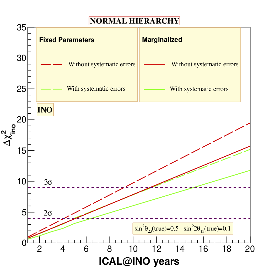
The atmospheric neutrino fluxes have large systematic uncertainties. In order to study the impact of these systematic uncertainties on the projected reach of ICAL@INO to the neutrino mass hierarchy, we show in Fig. 8 the mass hierarchy sensitivity with and without systematic uncertainties in the ICAL@INO analysis. The $\Delta\chi^{2}$ is shown as a function of the number of years of exposure of the experiment. The data was generated at the benchmark oscillation point. The red lines are obtained without taking systematic uncertainties in the ICAL@INO analysis, while the green lines are obtained when systematic uncertainties are included. The long-dashed lines are for fixed parameters in theory as in the data, while the solid lines are obtained by marginalizing over $|\Delta m^{2}_{\rm eff}|$, $\sin^{2}\theta_{23}$ and $\sin^{2}2\theta_{13}$. The left panel is for true normal hierarchy while the right panel is for true inverted hierarchy. The effect of taking systematic uncertainties is to reduce the statistical significance of the analysis. We have checked that of the five systematic uncertainties, the uncertainty on overall normalization of the fluxes and the cross-section normalization uncertainty have minimal impact on the final results. The reason for that can be understood from the fact that the atmospheric neutrinos come from all zenith angles and over a wide range of energies. The overall normalization uncertainty is the same for all bins, while the mass hierarchy dependent earth matter effects, are important only in certain zenith angle bin and certain range of energies. Therefore, the effect of the overall normalization errors get cancelled between different bins. On the other hand, the tilt error could be used to modify the energy spectrum of the muons in the fit and the zenith angle error allows changes to the zenith angle distribution. Therefore, these errors do not cancel between the different bins and can dilute the significance of the data. In particular, we have checked that the effect of the zenith angle dependent systematic error on the atmospheric neutrino fluxes has the maximum effect on the lowering of the $\Delta\chi^{2}$ for the mass hierarchy sensitivity.

It is well known that the amount of earth matter effects increases with increase in both $\theta_{13}$ and $\theta_{23}$. In the previous plots, we showed the mass hierarchy sensitivity for different allowed values of $\sin^{2}2\theta_{13}{\mbox{(true)}}$, while $\sin^{2}\theta_{23}{\mbox{(true)}}$ was fixed at maximal mixing. In Figs. 9 and 10 we show the sensitivity to the neutrino mass hierarchy as a function of number of years of running of ICAL@INO for different values of $\sin^{2}2\theta_{13}{\mbox{(true)}}$ as well as $\sin^{2}\theta_{23}{\mbox{(true)}}$. In Fig. 9 we show the $\Delta\chi^{2}$ corresponding to ICAL@INO alone and with oscillation parameters fixed in the fit at their true values. This figure corresponds to Fig. 5 of the previous section but now with two other values of $\sin^{2}\theta_{23}{\mbox{(true)}}$. In Fig. 10 we give the combined sensitivity to mass hierarchy of all accelerator and reactor experiments combined with the data of ICAL@INO. We reiterate that the $x$-axis of the Fig. 10 shows the exposure of ICAL@INO, while for all other experiments we have assumed the full run time as discussed in section 3.2. The red bands in Figs. 9 and 10 correspond to $\sin^{2}\theta_{23}{\mbox{(true)}}=0.6$ while the green bands are for $\sin^{2}\theta_{23}{\mbox{(true)}}=0.4$. The width of each of the bands is mapped by increasing the value of $\sin^{2}2\theta_{13}{\mbox{(true)}}$ from 0.08, through 0.1, and up to 0.12. As seen in the previous subsection, the $\Delta\chi^{2}$ for the wrong mass hierarchy increases with $\sin^{2}2\theta_{13}{\mbox{(true)}}$ for a given value of $\sin^{2}\theta_{23}{\mbox{(true)}}$ and ICAL@INO exposure. A comparison of the $\Delta\chi^{2}$ for different values of $\sin^{2}\theta_{23}{\mbox{(true)}}$ reveals that the $\Delta\chi^{2}$ also increases with $\sin^{2}\theta_{23}{\mbox{(true)}}$.

From Fig. 10 one infers that for $\delta_{CP}{\mbox{(true)}}=0$, a combined analysis of all relevant experimental data including 5 years of ICAL@INO exposure would give the neutrino mass hierarchy from anywhere between about $2\sigma$ to $3.8\sigma$, depending on the values of $\sin^{2}\theta_{23}{\mbox{(true)}}$ and $\sin^{2}2\theta_{13}{\mbox{(true)}}$. With 10 years of running of ICAL@INO this would improve to $2.3\sigma$ to $4.6\sigma$, depending on what value of $\sin^{2}2\theta_{13}{\mbox{(true)}}$ and $\sin^{2}\theta_{23}{\mbox{(true)}}$ have been chosen by mother Nature. Here we have allowed $\sin^{2}\theta_{23}{\mbox{(true)}}$ to vary between $[0.4-0.6]$ and $\sin^{2}2\theta_{13}{\mbox{(true)}}$ between $[0.08-0.12]$. We next look at the impact of $\delta_{CP}{\mbox{(true)}}$ on the prospects of determining the neutrino mass hierarchy.

So far we had taken $\delta_{CP}$(true)=0 in the data and varied $\delta_{CP}$ in the fit only for the long baseline experiments. For the analysis of the ICAL@INO data, we had kept $\delta_{CP}$ fixed to zero in both the data and the theory. The reason was that while the $\chi^{2}$ for T2K and NO$\nu$A are strongly dependent on $\delta_{CP}$, the mass hierarchy $\chi^{2}$ for ICAL@INO shows a very mild dependence on it. We show this dependence explicitly in Fig. 11 for 10 years exposure in ICAL@INO and compare it with the corresponding dependence of NO$\nu$A (see also [31])⁵⁵ 5 This figure was shown in [31]. However, the analysis in [31] was in terms of neutrinos done with some assumed values of the detector resolutions and efficiencies. Since we do here the complete analysis of the ICAL@INO projected data in terms of the detected muons and with realistic detector resolutions and efficiencies obtained from ICAL simulations, we reproduce a similar plot for completeness. . We generate the data for normal hierarchy and at the benchmark values of the oscillation parameters from Table 1 and with $\sin^{2}\theta_{23}{\mbox{(true)}}=0.5$ and $\sin^{2}2\theta_{13}{\mbox{(true)}}=0.1$. In the fit with inverted hierarchy, we keep all oscillation parameters fixed, except $\delta_{CP}$ which is varied over its full range $[0-2\pi]$. The corresponding $\Delta\chi^{2}$ is plotted in Fig. 11 as a function of the $\delta_{CP}$ in the fit. The red long-dashed line shows the $\delta_{CP}$ dependence of $\Delta\chi^{2}$ for ICAL@INO, while the blue solid line shows the wild fluctuation of $\Delta\chi^{2}$ expected for NO$\nu$A. Amongst the accelerator and reactor experiments we show only NO$\nu$A in this figure as the leading contribution to the mass hierarchy comes from this experiment. We reiterate that at each point we use the data generated at $\delta_{CP}$(true)=0. The figure shows that when we fit the data with inverted hierarchy, the $\Delta\chi^{2}$ for NO$\nu$A changes from more that 26 for $\delta_{CP}\simeq 80^{\circ}$ to less than 3 for $\delta_{CP}\simeq 260^{\circ}$. When marginalized over $\delta_{CP}$ in the fit, obviously it will return the lowest value of the $\Delta\chi^{2}$, which in this case would be 2.59 ⁶⁶ 6 Note that here the other parameters are fixed and only NO$\nu$A data is being considered in the analysis, while the $\Delta\chi^{2}$s shown in Table 2 are for a global fit of all data with all oscillation parameters allowed to vary freely in the fit and the combined $\chi^{2}$ marginalized over them.. When marginalized over all oscillation paremeters, the sensitivity further reduces to $\Delta\chi^{2}=1.77$. The contribution from ICAL@INO on the other hand is seen to be almost independent of $\delta_{CP}$. Note that such a figure was also shown in [55] for the ICAL@INO simulations. However, the analysis of the ICAL data has been improved since then and more types of systematic uncertainties introduced. This explains the change in the behavior of this plot with the dependence of the $\Delta\chi^{2}$ becoming flatter with $\delta_{CP}$. From this study we conclude that one does not need to marginalize over $\delta_{CP}$ for the ICAL@INO data. However, for the long baseline experiments a fine marginalization over this parameter is absolutely crucial, especially for mass hierarchy studies.

We had seen in Fig. 11 (and as is well known) that the long baseline experiments are very sensitive to $\delta_{CP}$. In that figure we were studying the impact of changing $\delta_{CP}$ in the fit for a particular $\delta_{CP}$(true) in the data. In particular, we had taken $\delta_{CP}$(true)=0. A pertinent question at this point is the following: what is the impact of $\delta_{CP}$(true) on the sensitivity of the experiments to the neutrino mass hierarchy? We present the answer to this question in Fig. 12, where we show the $\Delta\chi^{2}$ for the mass hierarchy sensitivity as a function of $\delta_{CP}$(true). To obtain these curves, we generate data for normal hierarchy at each value of $\delta_{CP}$(true) shown in the $x$-axis and then fit this data for inverted hierarchy by marginalizing over all oscillation parameters, including $\delta_{CP}$. The data were generated for the benchmark oscillation point given in Table 1, $\sin^{2}\theta_{23}{\mbox{(true)}}=0.5$ and $\sin^{2}2\theta_{13}{\mbox{(true)}}=0.1$. The exposure considered is 10 years of ICAL@INO and full run for all other experiments. The green solid line in this figure is for only NO$\nu$A, the blue short-dashed line is obtained when we combine NO$\nu$A, T2K and all the reactor data, while the red long-dashed line is what we get when the ICAL@INO data is also added to the long baseline and reactor data. As expected, the ICAL@INO data is almost completely independent of $\delta_{CP}$(true) and so is its projected sensitivity to the neutrino mass hierarchy. On the other hand, the reach of the NO$\nu$A experiment for determining the neutrino mass hierarchy is seen to be extremely sensitive to the value of $\delta_{CP}$(true). All our plots shown so far on the global mass hierarchy reach were done assuming $\delta_{CP}{\mbox{(true)}}=0$. We can see from the figure that indeed the statistical significance with which we could rule out the inverted mass hierarchy in this case is $3.4\sigma$, as discussed before. The $\Delta\chi^{2}$ for $\delta_{CP}{\mbox{(true)}}=0$ for NO$\nu$A is 1.77. However, this quickly falls to almost zero for $\delta_{CP}{\mbox{(true)}}\simeq[50^{\circ}-150^{\circ}]$. Thereafter, it rises sharply giving a $\Delta\chi^{2}=8.21$ around $\delta_{CP}{\mbox{(true)}}\simeq 270^{\circ}$, and then finally falls back to $\Delta\chi^{2}=1.77$ for $\delta_{CP}{\mbox{(true)}}=360^{\circ}$. When T2K and all reactor data are added, there is an improvement to the combined sensitivity due to constraint coming from the mismatch between the best-fit for different experiments. This is specially relevant in the $\delta_{CP}{\mbox{(true)}}\simeq[50^{\circ}-150^{\circ}]$ range where NO$\nu$A by itself gives no mass hierarchy sensitivity. However, once we add the T2K and reactor data to NO$\nu$A data, the $\Delta\chi^{2}$ of this combined fit in this region of $\delta_{CP}{\mbox{(true)}}$ increases to $\simeq 3.5$. The reason for this can be understood as follows. For the case where $\delta_{CP}{\mbox{(true)}}=72^{\circ}$, the best-fit for NO$\nu$A alone was $\delta_{CP}=234^{\circ}$, $\sin^{2}\theta_{23}=0.5$ and $\sin^{2}2\theta_{13}=0.1$. For this $\delta_{CP}{\mbox{(true)}}$, T2K data taken alone gave $\Delta\chi^{2}\simeq 0$ with best-fit at $\delta_{CP}=198^{\circ}$, $\sin^{2}\theta_{23}=0.52$ and $\sin^{2}2\theta_{13}=0.08$. A combined fit with all accelerator and reactor data gave best-fit at $\delta_{CP}=198^{\circ}$, $\sin^{2}\theta_{23}=0.48$ and $\sin^{2}2\theta_{13}=0.1$. This results in a contribution to the mass hierarchy $\Delta\chi^{2}=0.92$ from NO$\nu$A, $\Delta\chi^{2}=1.41$ from T2K and $\Delta\chi^{2}=1.1$ from reactors. That the reactor data return a $\Delta\chi^{2}$ contribution to the mass hierarchy sensitivity might appear strange at the outset since the combined fit given above has a best-fit $\sin^{2}2\theta_{13}=0.1$, and one usually does not expect the reactor data to depend on sign of $\Delta m^{2}_{31}$, $\delta_{CP}$ and $\sin^{2}\theta_{23}$. However, note that the reactor data depend on $|\Delta m^{2}_{31}|$ and what we use in our fits is $\Delta m^{2}_{\rm eff}$ given by Eq. (3) which is related to $\delta_{CP}$. Therefore, as discussed earlier in section 6, this subtlety regarding the choice of the definition of the neutrino mass hierarchy results in a small change in the best-fit $|\Delta m^{2}_{31}|$, which in turn results in a small $\Delta\chi^{2}$ contribution to the mass hierarchy from the reactor experiments. Finally, addition of the ICAL@INO data raises the $\Delta\chi^{2}$ by a constant amount for all values of $\delta_{CP}{\mbox{(true)}}$. Therefore, depending on $\delta_{CP}{\mbox{(true)}}$ the combined sensitivity to the neutrino mass hierarchy could range from $3.3\sigma$ (for $\delta_{CP}{\mbox{(true)}}=144^{\circ}$) to $4.4\sigma$ (for $\delta_{CP}{\mbox{(true)}}\simeq 270^{\circ}$). These numbers are for $\sin^{2}\theta_{23}{\mbox{(true)}}=0.5$ and $\sin^{2}2\theta_{13}{\mbox{(true)}}=0.1$ and will improve for larger values of these parameters.

In this paper we looked in detail at the prospects of determining the neutrino mass hierarchy with the data collected in the atmospheric neutrino experiment ICAL@INO. The atmospheric muon neutrino events before oscillations were simulated using the NUANCE based generator developed for ICAL@INO. To reduce Monte Carlo fluctuations 1000 years of exposure was used for generating the events. Since it takes very long for the generator to produce such a large event sample, we simulated the atmospheric events using the generator just once for no oscillations and used a reweighting algorithm to obtain the oscillated event sample for any set of oscillation parameters. The oscillated muon event spectrum was then folded with the muon reconstruction efficiencies, charge identification efficiencies, energy resolution and the zenith angle resolution functions obtained from ICAL simulations (which will appear elsewhere [33]) to obtain the reconstructed muon event spectrum in the detector. As ICAL is a magnetized calorimetric detector allowing an identification of $\mu^{-}$ and $\mu^{+}$ events, it has an edge over rival atmospheric neutrino experiments. We defined a $\chi^{2}$ function for Poissonian distribution for the errors in the ICAL@INO experiment taking into account systematic uncertainties expected in the experiment.

The data was generated for benchmark true values for the oscillation parameters and a given neutrino mass hierarchy and fitted with the wrong hierarchy. We showed the mass hierarchy sensitivity results with only ICAL@INO data for the analysis with fixed values of the oscillation parameters in the fit, as well as that obtained after marginalization over $|\Delta m^{2}_{\rm eff}|$, $\sin^{2}\theta_{23}$ and $\sin^{2}2\theta_{13}$ in their current $3\sigma$ ranges. We showed these results as a function of the exposure in ICAL@INO. From a comparison of the two results, we showed that the mass hierarchy sensitivity with ICAL@INO data deteriorates with the uncertainty in the measured value of $|\Delta m^{2}_{\rm eff}|$, $\sin^{2}\theta_{23}$ and $\sin^{2}2\theta_{13}$. These parameters will be rather accurately determined by the T2K, NO$\nu$A Double Chooz, RENO and Daya Bay experiments. Since INO is expected to start operation after these have finished their full projected run, it is meaningful to include their effect in a combined statistical analysis for the neutrino mass hierarchy. In order to take that into account, we simulated the data for these experiments using GLoBES with the experimental specifications mentioned in their respective Letter Of Intent and/or Detailed Project Report. The results on mass hierarchy sensitivity from the combined analysis of data from ICAL@INO along with that from T2K, NO$\nu$A, Double Chooz, RENO and Daya Bay was shown for benchmark values of the oscillation parameters and full marginalization over all oscillation parameters in the fit for the wrong mass hierarchy. We showed that marginalization over $\delta_{CP}$ is practically unessential for the ICAL@INO data. However, for the accelerator data it is absolutely crucial to marginalize over $\delta_{CP}$ due to the very strong dependence of the hierarchy sensitivity on this parameter in these experiments. We then generated the data at all values of $\delta_{CP}{\mbox{(true)}}$ and showed that the mass hierarchy sensitivity of ICAL@INO was independent of $\delta_{CP}{\mbox{(true)}}$, however, the sensitivity of the combined NO$\nu$A, T2K and the reactor experiments depends very strongly on what $\delta_{CP}{\mbox{(true)}}$ has been chosen by Nature. For $\sin^{2}\theta_{23}{\mbox{(true)}}=0.5$ and $\sin^{2}2\theta_{13}{\mbox{(true)}}=0.1$ the combined data of 10 years exposure in ICAL@INO along with T2K, NO$\nu$A and reactor experiments could rule out the wrong hierarchy with a statistical significance of $3\sigma$ to $4.2\sigma$, depending on the chosen value of $\delta_{CP}{\mbox{(true)}}$. We also studied the effect of $\sin^{2}2\theta_{13}$(true) and $\sin^{2}\theta_{23}$(true) on the reach of these combined projected data sets to determining the neutrino mass hierarchy. For $\delta_{CP}{\mbox{(true)}}=0$, we showed that the statistical significance with which the wrong hierarchy could be ruled out by the global data set comprising of 10 years exposure in ICAL@INO along with T2K, NO$\nu$A and reactor experiments, could be anywhere between $2.13\sigma$ to $4.5\sigma$ depending on $\sin^{2}\theta_{23}{\mbox{(true)}}$ and $\sin^{2}2\theta_{13}$, where we allowed $\sin^{2}\theta_{23}{\mbox{(true)}}$ to vary between $[0.4-0.6]$ and $\sin^{2}2\theta_{13}{\mbox{(true)}}$ between $[0.08-0.12]$. For the most favorable choice of $\delta_{CP}{\mbox{(true)}}\simeq 270^{\circ}$ the sensitivity could go up to greater than $5\sigma$ with 10 years of ICAL@INO combined with data from T2K, NO$\nu$A and reactor experiments.

The first row of Table 2 shows the $\Delta\chi^{2}$ for the case used in this paper where normal hierarchy is defined as $\Delta m^{2}_{\rm eff}>0$ and inverted hierarchy is defined as $\Delta m^{2}_{\rm eff}<0$. In this case the survival probability $P_{{\nu_{\mu}}{\nu_{\mu}}}$ is almost the same for the normal and inverted hierarchies when $\theta_{13}=0$. However, this is not true for the channels $P_{{\nu_{\mu}}{\nu_{e}}}$ relevant for T2K and NOvA and $P_{{\nu_{e}}{\nu_{e}}}$ relevant for the reactor experiments. Thus in the best-fit, the value of $|\Delta m^{2}_{31}|$ and $\delta_{CP}$ has to be suitably adjusted so that the oscillation probabilities in these oscillation channels are closest to each other in the data and in the fit. This results in a small $\Delta\chi^{2}$ from experiments that by themselves have practically no hierarchy sensitivity at all. We have indeed checked that the $\Delta\chi^{2}$ for mass hierarchy is zero for all reactor experiments and T2K, when the fit is performed using data from only one experiment at a time and all oscillation parameters allowed to vary in the fit. Only when one performs a combined analysis does this tension between choice of the oscillation frequencies arise, returning a small contribution to the mass hierarchy from the reactor experiments and T2K.

References

- [1] K. Abe et al. [T2K Collaboration], Phys. Rev. Lett. 107, 041801 (2011) [arXiv:1106.2822 [hep-ex]].
- [2] P. Adamson et al. [MINOS Collaboration], Phys. Rev. Lett. 107, 181802 (2011) [arXiv:1108.0015 [hep-ex]].
- [3] Y. Abe et al. [DOUBLE-CHOOZ Collaboration], Phys. Rev. Lett. 108, 131801 (2012) [arXiv:1112.6353 [hep-ex]].
- [4] F. P. An et al. [DAYA-BAY Collaboration], Phys. Rev. Lett. 108, 171803 (2012) [arXiv:1203.1669 [hep-ex]].
- [5] J. K. Ahn et al. [RENO Collaboration], Phys. Rev. Lett. 108, 191802 (2012) [arXiv:1204.0626 [hep-ex]].
- [6] D. Ishitsuka [for the Double Chooz Collaboration]; D. Dwyer [for the Daya Bay Collaboration]; S. B. Kim [for the RENO Collaboration]; Talks at Neutrino 2012, the XXV International Conference on Neutrino Physics and Astrophysics (Kyoto, Japan, 2012), website: neu2012.kek.jp
- [7] M. C. Gonzalez-Garcia, M. Maltoni, J. Salvado and T. Schwetz, arXiv:1209.3023 [hep-ph].
- [8] G. L. Fogli, E. Lisi, A. Marrone, D. Montanino, A. Palazzo and A. M. Rotunno, Phys. Rev. D 86, 013012 (2012) [arXiv:1205.5254 [hep-ph]].
- [9] D. V. Forero, M. Tortola and J. W. F. Valle, arXiv:1205.4018 [hep-ph].
- [10] H. Minakata, arXiv:1209.1690 [hep-ph].
- [11] E. Fernandez-Martinez, talk at “What is ?, INVISIBLES 12 and Alexei Smirnov Fest”, GGI, Firenze, June, 2012.
- [12] J. Bernabeu, S. Palomares-Ruiz, A. Perez and S. T. Petcov, Phys. Lett. B 531, 90 (2002) [hep-ph/0110071].
- [13] M. C. Gonzalez-Garcia and M. Maltoni, Eur. Phys. J. C 26, 417 (2003) [hep-ph/0202218].
- [14] J. Bernabeu, S. Palomares Ruiz and S. T. Petcov, Nucl. Phys. B 669, 255 (2003) [hep-ph/0305152].
- [15] O. L. G. Peres and A. Y. .Smirnov, Nucl. Phys. B 680, 479 (2004) [hep-ph/0309312].
- [16] S. Palomares-Ruiz and S. T. Petcov, Nucl. Phys. B 712, 392 (2005) [hep-ph/0406096].
- [17] D. Indumathi and M. V. N. Murthy, Phys. Rev. D 71, 013001 (2005) [hep-ph/0407336].
- [18] R. Gandhi, P. Ghoshal, S. Goswami, P. Mehta and S. U. Sankar, Phys. Rev. D 73, 053001 (2006) [hep-ph/0411252].
- [19] S. Choubey and P. Roy, Phys. Rev. D 73, 013006 (2006) [hep-ph/0509197].
- [20] S. T. Petcov and T. Schwetz, Nucl. Phys. B 740, 1 (2006) [hep-ph/0511277].
- [21] D. Indumathi, M. V. N. Murthy, G. Rajasekaran and N. Sinha, Phys. Rev. D 74, 053004 (2006) [hep-ph/0603264].
- [22] S. Choubey, Nucl. Phys. Proc. Suppl. 221, 46 (2011) [hep-ph/0609182].
- [23] E. K. Akhmedov, M. Maltoni and A. Y. .Smirnov, JHEP 0705, 077 (2007) [hep-ph/0612285].
- [24] R. Gandhi, P. Ghoshal, S. Goswami, P. Mehta, S. U. Sankar and S. Shalgar, Phys. Rev. D 76, 073012 (2007) [arXiv:0707.1723 [hep-ph]].
- [25] E. K. .Akhmedov, M. Maltoni and A. Y. .Smirnov, JHEP 0806, 072 (2008) [arXiv:0804.1466 [hep-ph]].
- [26] R. Gandhi, P. Ghoshal, S. Goswami and S. U. Sankar, Phys. Rev. D 78, 073001 (2008) [arXiv:0807.2759 [hep-ph]].
- [27] A. Samanta, Phys. Rev. D 81, 037302 (2010) [arXiv:0907.3540 [hep-ph]].
- [28] A. Samanta and A. Y. .Smirnov, JHEP 1107, 048 (2011) [arXiv:1012.0360 [hep-ph]].
- [29] M. C. Gonzalez-Garcia, M. Maltoni and J. Salvado, JHEP 1105, 075 (2011) [arXiv:1103.4365 [hep-ph]].
- [30] V. Barger, R. Gandhi, P. Ghoshal, S. Goswami, D. Marfatia, S. Prakash, S. K. Raut and S U. Sankar, Phys. Rev. Lett. 109, 091801 (2012) [arXiv:1203.6012 [hep-ph]].
- [31] M. Blennow and T. Schwetz, JHEP 1208, 058 (2012) [arXiv:1203.3388 [hep-ph]].
- [32] D. Casper, webpage: nuint.ps.uci.edu/nuance/default.htm
- [33] “Simulations study of the sensitivity of the ICAL detector to muons”, INO Collaboration, under preparation.
- [34] “Hadron energy resolution at ICAL”, INO Collaboration, under preparation.
- [35] P. Huber, M. Lindner, T. Schwetz and W. Winter, JHEP 0911, 044 (2009) [arXiv:0907.1896 [hep-ph]].
- [36] B. T. Cleveland, T. Daily, R. Davis, Jr., J. R. Distel, K. Lande, C. K. Lee, P. S. Wildenhain and J. Ullman, Astrophys. J. 496, 505 (1998); F. Kaether, W. Hampel, G. Heusser, J. Kiko and T. Kirsten, Phys. Lett. B 685, 47 (2010) [arXiv:1001.2731 [hep-ex]]; J. N. Abdurashitov et al. [SAGE Collaboration], Phys. Rev. C 80, 015807 (2009) [arXiv:0901.2200 [nucl-ex]]; J. Hosaka et al. [Super-Kamiokande Collaboration], Phys. Rev. D 73, 112001 (2006) [hep-ex/0508053]; B. Aharmim et al. [SNO Collaboration], arXiv:1109.0763 [nucl-ex]; G. Bellini et al. [ The Borexino Collaboration], Phys. Rev. Lett. 107, 141302 (2011) [arXiv:1104.1816 [hep-ex]].
- [37] A. Gando et al. [KamLAND Collaboration], Phys. Rev. D 83, 052002 (2011) [arXiv:1009.4771 [hep-ex]].
- [38] Y. Itow [for the Super-Kamiokande Collaboration]; Talk at Neutrino 2012, the XXV International Conference on Neutrino Physics and Astrophysics (Kyoto, Japan, 2012), website: neu2012.kek.jp
- [39] R. Nichol [for the MINOS Collaboration]; Talk at Neutrino 2012, the XXV International Conference on Neutrino Physics and Astrophysics (Kyoto, Japan, 2012), website: neu2012.kek.jp
- [40] R. Gandhi, P. Ghoshal, S. Goswami and S U. Sankar, Mod. Phys. Lett. A 25 (2010) 2255 [arXiv:0905.2382 [hep-ph]].
- [41] H. Nunokawa, S. J. Parke and R. Zukanovich Funchal, Phys. Rev. D 72, 013009 (2005) [hep-ph/0503283].
- [42] K. Abe, T. Abe, H. Aihara, Y. Fukuda, Y. Hayato, K. Huang, A. K. Ichikawa and M. Ikeda et al., arXiv:1109.3262 [hep-ex].
- [43] A. Bueno, Z. Dai, Y. Ge, M. Laffranchi, A. J. Melgarejo, A. Meregaglia, S. Navas and A. Rubbia, JHEP 0704, 041 (2007) [hep-ph/0701101].
- [44] A. Ereditato and A. Rubbia, Nucl. Phys. Proc. Suppl. 155, 233 (2006) [hep-ph/0510131].
- [45] D. J. Koskinen, Mod. Phys. Lett. A 26, 2899 (2011).
- [46] E. K. .Akhmedov, S. Razzaque and A. Y. .Smirnov, arXiv:1205.7071 [hep-ph].
- [47] P. Huber, J. Kopp, M. Lindner, M. Rolinec and W. Winter, Comput. Phys. Commun. 177, 432 (2007) [hep-ph/0701187]; P. Huber, M. Lindner and W. Winter, Comput. Phys. Commun. 167, 195 (2005) [hep-ph/0407333].
- [48] F. Ardellier, I. Barabanov, J. C. Barriere, M. Bauer, L. B. Bezrukov, C. .Buck, C. Cattadori and B. Courty et al., hep-ex/0405032.
- [49] J. K. Ahn et al. [RENO Collaboration], arXiv:1003.1391 [hep-ex].
- [50] X. Guo et al. [Daya-Bay Collaboration], hep-ex/0701029.
- [51] Y. Itow et al. [T2K Collaboration], hep-ex/0106019.
- [52] D. S. Ayres et al. [NOvA Collaboration], hep-ex/0503053.
- [53] M. Honda, T. Kajita, K. Kasahara and S. Midorikawa, Phys. Rev. D 70, 043008 (2004) [astro-ph/0404457].
- [54] M. S. Athar, M. Honda, T. Kajita, K. Kasahara and S. Midorikawa, arXiv:1210.5154 [hep-ph].
- [55] S. Choubey, Talk at Neutrino 2012, the XXV International Conference on Neutrino Physics and Astrophysics (Kyoto, Japan, 2012), website: neu2012.kek.jp ; A. Dighe, Talk at NuFact 2012 14th International Workshop on Neutrino Factories, Super Beams and Beta Beams (Williamsburg, Virginia, USA, 2012), website: www.jlab.org/indico/conferenceDisplay.py?confId=0 ; S. Goswami, Talk at NOW 2012 Neutrino Oscillation Workshop (Otranto, Lecce, Italy, 2012), website: www.ba.infn.it/ now/now2012/web-content/index.html