THE CLUSTERING OF GALAXIES IN THE SDSS-III BARYON OSCILLATION SPECTROSCOPIC SURVEY: LUMINOSITY AND COLOR DEPENDENCE AND REDSHIFT EVOLUTION
Abstract
We measure the luminosity and color dependence and the redshift evolution of galaxy clustering in the Sloan Digital Sky Survey-III Baryon Oscillation Spectroscopic Survey Ninth Data Release. We focus on the projected two-point correlation function (2PCF) of subsets of its CMASS sample, which includes about galaxies over in the redshift range . To minimize the selection effect on galaxy clustering, we construct well-defined luminosity and color subsamples by carefully accounting for the CMASS galaxy selection cuts. The 2PCF of the whole CMASS sample, if approximated by a power-law, has a correlation length of and an index of . Clear dependences on galaxy luminosity and color are found for the projected 2PCF in all redshift bins, with more luminous and redder galaxies generally exhibiting stronger clustering and steeper 2PCF. The color dependence is also clearly seen for galaxies within the red sequence, consistent with the behavior of SDSS-II main sample galaxies at lower redshifts. At a given luminosity (k+e corrected), no significant evolution of the projected 2PCFs with redshift is detected for red sequence galaxies. We also construct galaxy samples of fixed number density at different redshifts, using redshift-dependent magnitude thresholds. The clustering of these galaxies in the CMASS redshift range is found to be consistent with that predicted by passive evolution. Our measurements of the luminosity and color dependence and redshift evolution of galaxy clustering will allow for detailed modeling of the relation between galaxies and dark matter halos and new constraints on galaxy formation and evolution.
Subject headings
cosmology: observations — cosmology: theory — galaxies: distances and redshifts — galaxies: halos — galaxies: statistics — large-scale structure of universeI. Introduction
Galaxies in the universe are observed to display a wide range of properties, such as luminosity, color, stellar mass, age, morphology, and spectral type. These properties encode information about galaxy formation and evolution and are related to the environment hosting the galaxies. Different populations of galaxies are thus expected to trace the underlying dark matter distribution in different ways.
Contemporary galaxy redshift surveys, most notably the Sloan Digital Sky Survey (SDSS; York et al. 106), have transformed the study of large-scale structure, enabling pristine measurements and detailed studies of galaxy clustering. Galaxy clustering provides a powerful approach to probe the complex relation between galaxies and the underlying dark matter distribution [41, e.g.,]. The dependence of galaxy clustering on galaxy properties has been observed in numerous galaxy surveys [21, 22, 38, 49, 5, 37, 61, 62, 107, 110, 111, 11, 50, 47, 15, 16, 55, 56, 97, 98, 92, 57, 68, 86, 48, 70, 73, 99, 14, 59, e.g.,].
In general, more luminous and redder galaxies are found to be more strongly clustered than their fainter and bluer counterparts. Similarly, early-type (elliptical) galaxies exhibit stronger clustering than late-type (spiral) ones. Galaxy luminosity and color are perhaps the two major readily observed properties, which also facilitate comparison between different surveys and are less dependent on the stellar evolution models. Moreover, they have proven to be the two properties most predictive of galaxy environment, such that any residual dependence on morphology or surface brightness is weak [8]. In this paper, we measure the dependence of galaxy clustering on color and luminosity for galaxies in the SDSS-III Baryon Oscillation Spectroscopic Survey (BOSS; Eisenstein et al. 27, Dawson et al. 24) and study the implications.
Galaxy clustering measurements, once properly interpreted, can provide key information about galaxy formation and evolution. In particular, the theoretical understanding of galaxy clustering has been greatly advanced with the development of dark matter halo models (see Cooray & Sheth 20 and references therein). In the cosmological constant + cold dark matter (CDM) paradigm, galaxies form and evolve in dark matter halos. While the properties and clustering of dark matter halos are well understood with the help of analytic models and numerical simulations [58, 89, e.g.,], the properties of galaxies are hard to predict because of the complex baryonic processes and the lack of complete theory of galaxy formation.
Galaxy clustering offers an opportunity to connect galaxies to dark matter halos, providing a new direction in studying galaxy formation and evolution. The halo occupation distribution (HOD) framework [66, 82, 79, 6, 7, 114, see e.g.,] or the closely related conditional luminosity function (CLF) method [105, 104] describe the number of galaxies as a function of halo mass, and galaxy clustering is used to constrain the HOD or CLF parameters. The subhalo abundance matching method makes use of subhalos in high resolution -body simulations and connects them to galaxies to interpret galaxy clustering [45, 19, 36, 63, see, e.g.,]. Such models essentially convert galaxy clustering measurements to the relation between galaxies and halos, which provides strong tests of galaxy formation models.
The galaxy-halo connections inferred at different redshifts, together with the theoretically known halo evolution, can lead to empirical constraints on galaxy evolution. For example, [112] compare the HODs for DEEP2 and SDSS galaxies and find a halo mass dependent growth of stellar mass of central galaxies, separating into contributions from star formation and mergers. [93] analyze four samples of galaxies from redshift to . They find that more than of the red satellite galaxies move onto the red sequence because of halo mergers, while the mechanism for central galaxies to move to the red sequence evolves from to .
To advance our understanding of galaxy evolution, improved measurements of galaxy clustering in large galaxy surveys at different redshifts are necessary. The color and luminosity dependence of clustering has been studied in detail at for DEEP2 galaxies [16] and at for SDSS galaxies (Zehavi et al. 111; denoted Z11 hereafter). The trends with color and luminosity are generally similar. However, while [16] find no changes of the clustering within the red sequence, Z11 find a continuous trend (in both amplitude and slope) of stronger clustering with color in SDSS galaxies. This discrepancy may be caused by different sample selections, but it may also be a signature of galaxy evolution (e.g., related to the buildup of red sequence). Studying a sample from an intermediate redshift range can provide new important information and a better understanding of galaxy evolution.
In this paper, we use the recently released CMASS sample of the BOSS Data Release 9 (DR9; Ahn et al. 1) to measure the clustering of galaxies in the redshift range and study the dependence on galaxy luminosity and color. The sample is constructed to contain a roughly volume-limited set of massive and luminous galaxies (with a typical stellar mass of ; Maraston et al. 52) in this redshift range. This sample has recently been used to accurately measure the baryon acoustic oscillation (BAO) signature (see Weinberg et al. 100 for a recent comprehensive review) on large scales () by Anderson et al. [2]. The sample has been thoroughly vetted, and the robustness of the results and cosmological constraints from the BAO and redshift-space distortions are explored in a series of papers [67, 72, 71, 76, 75, 80, 95, 96]. The smaller scale clustering measurements and HOD fits are first presented by White et al. [103] (for an earlier smaller sample) and Nuza et al. [63]. Here we study the small to intermediate scale (0.05–25) two-point correlation functions (2PCFs) of CMASS galaxies, focusing especially on the dependence on luminosity and color and the implications on galaxy evolution from simple models. We will study the evolution of CMASS galaxies based on HOD modeling in a companion paper.
The structure of the paper is organized as follows. In Section II, we briefly describe the CMASS sample and our method of measuring the 2PCFs. The division to specific subsamples, the clustering measurements and detailed dependence on luminosity and color, and the implications for galaxy evolution are presented in Section III. We summarize our results in Section IV. Appendix A discusses the effect of different stellar evolution models on our results, and Appendix B explores the robustness of the jackknife error estimates used.
Throughout the paper, we assume a spatially flat CDM cosmology as in Anderson et al. [2], with , , , , and , consistent with the best-fit model from the Wilkinson Microwave Anisotropy Probe 7-year data [44].
II. Observations and Methods
II.1. Data
As part of the SDSS-III survey, BOSS selects luminous galaxies from the multiple-band SDSS imaging [31, 33, 34, 106] for spectroscopic observation to probe the large-scale BAO signals [2]. [24] provide a comprehensive overview of BOSS, while the technical details of BOSS are presented in [87] and [9]. The selection of BOSS galaxies is a union of targets in two different redshift intervals. One is an extension of the SDSS-I/II Luminous Red Galaxy (LRG) sample [26], referred to as LOWZ with [65]. The other, denoted as CMASS [103, 2], includes galaxies in DR9, and is approximately stellar-mass limited at higher redshifts () with an effective volume of and an effective area of about . In this paper, our study focuses on the CMASS sample. The target selection cuts for CMASS galaxies are fainter and bluer than the LRG sample in order to achieve a higher number density of about and sample a wider range of galaxies. The detailed target selection of the CMASS sample is described in [64], and summarized in [27] and [2]. We briefly describe here the major selection cuts that will affect our analysis of luminosity and color dependence of the 2PCF.
The CMASS sample aims at selecting galaxies following a roughly constant stellar mass cut at redshift . The selection criteria of the CMASS galaxies are defined by,
| (1) | |||||
| (2) | |||||
| (3) | |||||
| (4) | |||||
| (5) |
where is defined as
| (6) |
and all magnitudes are extinction corrected [78] and are in the observed frame. While the magnitudes are calculated using cmodel magnitudes (denoted by the subscript “cmod”), the colors are computed using model magnitudes (denoted by the subscript “mod”; see Anderson et al. 2 for details). The magnitude corresponds to the -band flux within the fiber size. CMASS objects also pass specific star-galaxy separation cuts, as described in [2].
II.2. Selection Cuts and Sample Completeness

The CMASS galaxies are chosen by applying complex target selection cuts, and it is thus difficult to construct exact volume-limited samples. Since we intend to investigate the luminosity and color dependence of galaxy clustering in this paper, we must pay particular attention to the completeness in luminosity and color. With this goal in mind, we first investigate the target selection cuts projected to the color-luminosity plane at different redshifts, which will provide the appropriate boundaries in constructing our samples.
Figure 1 shows the color-magnitude diagram (CMD) at six narrow redshift ranges with . The contours represent the number density distribution of CMASS galaxies in the CMD. The absolute magnitude and color are k+e corrected to throughout the paper using a global Flexible Stellar Population Synthesis (FSPS) model [18, 17, 94, 96]. Using other stellar evolution models slightly changes the resulting magnitudes and colors, but does not affect our analysis of galaxy clustering, as we discuss in Appendix A. In each panel of Figure 1, only the approximate positions of the selection cuts are shown as dashed lines, since the selection cuts are made in apparent magnitudes and in three bands ( and, ) while our CMD is shown for color and magnitude. The slopes of the dashed lines follow the boundaries seen in the CMD contours in each redshift bin. We focus on the three main cuts (Equations 1–3). Following [111], we adopt a luminosity-dependent color cut to separate red and blue galaxies (discussed in detail in Section III.3),
| (7) |
represented by the green lines in Figure 1.
The horizontal cut in each panel corresponds to the -band faint-end flux limit (Equation 1, ), which selects galaxies brighter than the corresponding absolute magnitude at each redshift. The slightly tilted vertical dashed line on the left of the distribution is the cut (Equation 2), which removes galaxies with bluer colors and with lower redshifts [12, 64]. The bottom-left dashed line is the -band sliding cut (Equation 3), which excludes the fainter and bluer (thus lower stellar mass) galaxies from the sample. These three main cuts evolve with redshift. A consequence of the and sliding cuts is that there are more blue galaxies at higher redshifts. At , while the CMASS sample is less affected by the cut, the sliding cut must be carefully taken into account at all redshifts in constructing complete galaxy samples. At , blue galaxies are highly incomplete (see an estimation of the fraction of star-forming galaxies in CMASS in Figure 16 of Chen et al. 13). At , the cut leads to incompleteness even for the most luminous red galaxies.
A more sophisticated method to study the sample completeness would be to simulate the galaxy properties (stellar mass, luminosity and color) at different redshifts by assuming certain galaxy stellar evolution models and to apply the selection cuts to simulated galaxies [91]. While it would generally depend on the assumptions in the galaxy evolution models, such a study can provide a quantitative estimate of the sample completeness as a function of color and luminosity. In this paper, however, we do not intend to evoke such a model in our clustering analysis. Instead, we empirically use the CMD and selection cuts at each redshift to construct approximately complete galaxy samples. As we proceed in our analysis, we keep in mind the boundaries of “completeness” defined by the selection cuts when constructing our galaxy samples. One advantage of such an empirical method is that it is largely model-independent.
II.3. Clustering Measurements
In this paper, we focus our discussion on the galaxy 2PCF. We use the Landy-Szalay estimator [46] to measure the 2PCF of galaxies,
| (8) |
where , and are the data–data, data–random, and random–random pair counts measured from the data of galaxies and random samples consisting of random points. These pair counts are appropriately normalized by , , and , respectively.
We measure the three-dimensional (3D) 2PCF , where and are the separations of galaxy pairs perpendicular and parallel to the line of sight. The redshift-space 2PCF differs from the real-space one because of redshift distortions induced by galaxy peculiar velocities. The redshift distortions can be mitigated by projecting the 2PCF along the line-of-sight direction, with the projected 2PCF [23] defined and measured as
| (9) |
where and are the –th bin of the line-of-sight separation and its corresponding bin size. In practice, we sum along the line-of-sight direction up to to include most of the correlated pairs. As our analysis focuses on 2PCF measurements up to , the clustering measurements do not depend significantly on the assumed once it is sufficiently larger. For example, if we integrate the line-of-sight direction to , the contribution from to only introduces noisy fluctuations of about .
The projected 2PCF can be related to the real-space correlation function, , by
| (10) |
[23]. It is common practice to characterize by a power law on small scales, , and in such a case can be expressed as
| (11) |
The covariance matrix of the correlation function is estimated using the jackknife resampling method (following Zehavi et al. 110, Zehavi et al. 111)
| (12) |
where is the total number of jackknife samples, is the 2PCF in the –th pair separation bin measured from the –th jackknife sample, and is the average over all samples. We expand on the tests performed by [110] and investigate the accuracy of the jackknife error estimates using CMASS mock catalogs and find good agreement between the jackknife estimates and those from multiple mocks (see Appendix B for more details).
We focus on analyzing our measurement of the galaxy 2PCF on the small to intermediate scales (), aiming at probing the relation between galaxies and their host halos. However, the small-scale measurement of the 2PCF is limited by the fiber collision effect in the spectrograph system of SDSS-III, where two fibers on the same plate cannot be placed closer than an angular separation of [24, 2]. As a result, about of CMASS galaxies do not have redshifts, strongly affecting small-scale clustering measurements. We correct for this effect using the method proposed and tested by [35], which divides the galaxy sample into two distinct populations, one free of fiber collisions (referred to as ) and the other consisting of potentially collided galaxies (denoted as ). The total clustering signal is a combination of the contributions from these two populations, where the contribution of the collided population is estimated from the resolved galaxies in tile-overlap regions.
As discussed in detail in [35], there are two main systematics that could impact the accuracy of such a method to treat fiber collisions. One is possible density variations between the tile overlap and non-overlap regions, which is found to be insignificant from tests with mock galaxy catalogs. Another effect is that galaxies in collided triplets (or even higher-order colliding groups) can only be fully recovered in regions covered by at least three tiles, making the estimation from close pairs in two-tile regions not accurate (because of the lack of close pairs). This effect is alleviated by an additional correction term using the measured close pairs in the two-tile regions. After full application of the [35] method, we estimate the remaining systematic errors to be less than 3–5%. It is generally difficult to have an unbiased correction on all scales, but this approach provides the best estimate of the galaxy 2PCF on small scales, compared with other possible methods.
When counting pairs for the 2PCF, each galaxy is assigned a series of weights to reduce variance in the measurements and take into account different effects. Following [2], we apply a scale-independent weight to optimize the clustering measurements [29]
| (13) |
where is the mean density at redshift , and . This equation provides similar results to the minimum variance weight used by [39] and [107]. Another employed weight, , accounts for the fact that not every galaxy with a spectrum taken has a reliable redshift measurement. The “redshift failures” are dependent on the positions of fibers on the plates [72] and are corrected by up-weighting the nearest galaxy that has an accurate redshift. The final weight, , is caused by the scarcity of galaxies detected due to foreground bright stars [73]. [72] present a comprehensive study of potential systematic effects in the 2PCF analysis, and compute a set of weights based on the stellar density and magnitude. Therefore, the total weight applied to each galaxy is
| (14) |
The quantity is applied to both the and populations in the fiber collision correction. The systematic weight only has a small effect on small and intermediate scales, but significantly changes the clustering measurements on BAO scales.
We construct the random catalogs according to the detailed angular selection of the DR9 galaxy sample. The radial selection function for each sample is taken into account by assigning the shuffled galaxy redshifts to the random objects. The shuffling method provides a better representation of the true distribution compared with a smooth spline fit to the observed galaxy redshift distribution, as detailed in [72]. This process is done separately for the northern and southern Galactic Caps to account for the different number density distributions [see 2, for details]. To apply the fiber collision correction, separate random catalogs for the and populations are used. Denoting the fraction of recovered galaxies as , for the random catalogs we apply an additional angular mask in each sector (see Guo et al. 35 for details).
III. Results
III.1. 2PCF of the Full CMASS Sample

Before presenting the luminosity and color dependence of the 2PCFs for CMASS galaxies, we show in Figure 2 the projected and redshift-space 2PCFs for the entire CMASS sample in the redshift range (solid lines). For comparison, we also display the recent CMASS DR9 measurements of Nuza et al. [63, open symbols], which are limited to slightly larger scales () and show good agreement on all measured scales. The vertical dashed lines indicate the maximal fiber collision scale, at redshift . By applying the fiber-collision correction method of [35], we are able to robustly measure the small-scale clustering (note the small error bars). This should enable better constraints on the spatial distribution of galaxies inside dark matter halos and a better constraint on the fraction of satellite galaxies, which we will address in future work.
The dotted line in the left panel of Figure 2 is the power-law fit to for , based on Equation 11, using the full error covariance matrix. Although clearly deviates from a power-law (also shown from the of the fitting), a power-law fit provides a simple characterization of the clustering and allows for easy comparisons among the 2PCFs of different galaxy samples. The correlation length for the CMASS sample is and the slope (note that given the large bestfit , the error bars here should be interpreted with care). These values are similar to clustering measurements of LRGs at from the 2dF-SDSS LRG and QSO (2SLAQ) survey [12, 74, 98], as expected, since the CMASS galaxy color selections were based on the 2SLAQ LRG selection.
In order to study the large-scale galaxy bias, we focus on scales larger than typical dark matter halo sizes. By fitting the ratio between the measured galaxy and the theoretically computed dark matter on scales (detailed in Section III.5), we obtain a “large-scale” galaxy bias factor of , consistent with the measurements of other authors [103, 63, 76, 83]. The galaxy bias determined from the projected 2PCF has less scale dependence than that from the redshift-space 2PCF. The exact value of the implied bias can depend on the fitting scales and fitting methods. We find that if the minimal fitting scale is changed from to (or larger), the resulting bias only varies slightly at the level. In the right panel of Figure 2 we present the redshift-space 2PCF on scales above , where it can be reliably measured. The fiber collisions in that case impact larger scales than indicated by the dashed line, since includes the contribution from the line-of-sight separations, (see more discussion in Guo et al. 35).
III.2. Luminosity Dependence
III.2.1 Luminosity Cuts

We now investigate the luminosity dependence of CMASS galaxy clustering. To minimize the influence of sample incompleteness, we carefully construct samples of different luminosities by accounting for the selection cuts as a function of redshifts discussed in Section II.2. We divide galaxies into two redshift bins, and . The color-magnitude distributions in these two redshift bins, the overall magnitude-redshift distribution, and the cuts used to define our samples are shown in Figure 3. In the right-most panel, some galaxies lie below the faint flux limit (denoted by the lower green line), reflecting the change between the photometry at the time of targeting and that from the final processing. To keep a uniform criterion, we construct our luminosity samples based on the targeting photometry [2, see details in]. We avoid the impact of the sliding cut by only selecting galaxies brighter than the intersections between the and sliding cuts. The incompleteness caused by the cut at cannot be avoided. Such a limitation means that the blue galaxies are incomplete, especially for the low-redshift samples, while the red galaxies are close to complete for , which is a caveat to remember when interpreting the results. We will thus also study the luminosity dependence limited to the more complete red galaxies. The sliding cut also impacts our ability to study fainter galaxies at high redshift, resulting in the unsampled “triangle” region above in the right panel of Figure 3. We have three and two luminosity bin samples at lower and higher redshifts, respectively, each with a bin width of 0.3 magnitude, as shown in the figure.
| range | range | |||||||
|---|---|---|---|---|---|---|---|---|
| -21.9, -21.6 | 0.43, 0.55 | 48391 | 46235 | 2156 | 0.484 | 47.89/10 | ||
| -22.2, -21.9 | 0.43, 0.55 | 24190 | 22419 | 1771 | 0.484 | 45.87/10 | ||
| -22.5, -22.2 | 0.43, 0.55 | 9308 | 8687 | 621 | 0.484 | 10.22/10 | ||
| -22.5, -22.2 | 0.55, 0.70 | 23404 | 15821 | 7583 | 0.851 | 10.68/10 | ||
| -22.8, -22.5 | 0.55, 0.70 | 7484 | 5135 | 2349 | 0.851 | 15.13/10 |
Note. — and are obtained from fitting a power-law to using the full error covariance matrices for . The ratios between and degrees-of-freedom (dof) of the fits are also shown.
The total numbers of galaxies, , and the comoving volume, , in each luminosity bin are shown in Table 1. We also provide the number of blue and red galaxies using the color cut (Equation 7). Power-law fits of Equation 11 to the projected 2PCF for are also given in the table. It is evident that at lower redshifts, red galaxies dominate the samples, and blue galaxies contribute less than . At higher redshifts, approximately of the sample are blue galaxies. This could still be partly related to the CMASS selection effects. If the change in blue galaxy fraction is caused by evolution, i.e., blue galaxies turning red with time, we would expect the luminosity dependence of the 2PCF for red galaxies to also evolve with redshift.
III.2.2 The Dependence of Galaxy 2PCF on Luminosity

The projected 2PCFs of different luminosity samples at the two redshift bins are shown in the top panels of Figure 4. At both redshifts, the luminosity dependence of is evident, with more luminous galaxies exhibiting stronger clustering, consistent with the results of the SDSS-I/II main sample [110, 111, 47]. At , since red galaxies contribute of the CMASS galaxy population, the luminosity dependence mostly reflects the clustering environment of the red galaxies. At , our measurements of the 2PCF become noisier because of the lower number of galaxies. Even after accounting for the uncertainties in the measurements, the luminosity dependence of clustering is significant in the redshift range of CMASS galaxies.
According to the HOD modeling results in SDSS-I/II [110, 111], the increase in the clustering amplitude for more luminous samples reflects the shift in the host halo mass toward the high mass end. The modeling results in Zehavi et al. [110], Zehavi et al. [111] also show that the satellite fraction drops as the luminosity of galaxies increases. Our measurements naively seem to support such a result — although the 2PCFs becomes generally noisier for higher luminosity samples, the uncertainties in the 2PCFs on small scales increase faster. At such scales, satellite galaxies have a significant contribution to the clustering signal. Therefore, the increase in the measurement errors could be a reflection of the lack of satellites in more luminous samples.
The shapes of for all luminosity samples are similar. The deviation from a power-law in is somewhat more apparent for brighter galaxies, consistent with the results from main galaxies [108, 110, 111]. In the halo model, the slope of has a rapid change around a few Mpc, indicating the transition from intra-halo galaxy pairs (1-halo term) to inter-halo galaxy pairs (2-halo term). In our measurements, we see that this transition scale increases with increasing luminosity, in agreement with the interpretation that more luminous galaxies reside in more massive (hence larger) halos. The dotted lines in the top left panel of Figure 4 show the power-law fits to in the range of . There is an apparent weak trend that brighter galaxies have a steeper slope in on small scales, in line with the result in Z11. The dotted lines in the top left panel show the power-law fits to the in the range of , the slope varies from (the faintest sample) to (the brightest sample). The trend can also be interpreted as a result of the change in the host halo mass scale (see Figure 7 and Appendix A in Zheng et al. 113).
The bottom panels of Figure 4 show the redshift evolution of the 2PCFs of galaxies in a fixed luminosity bin . The left panel is for all the galaxies (both blue and red). Galaxies at a lower redshift appear to have a higher clustering strength. This result may be due to the incompleteness of blue galaxies at lower redshifts, and the inclusion of more (less clustered) blue galaxies at higher redshifts. We therefore also examine the redshift evolution of the 2PCF in the sample for red galaxies only, as shown in the bottom-right panel of Figure 4, where the red galaxies are defined by the color cut in Equation 7. We find only slight evolution with redshift for the red galaxies (at most in for ), not significant within the measurement errors, implying that the differences in the sample of all galaxies (bottom-left panel) are mostly induced by the blue galaxies.
In the redshift range of , [109] find no strong evolution trend in in the SDSS LRG sample. Their sample of at has a comoving number density of (their Figure 2), similar to the number density of our sample of at shown in the bottom right panel of Figure 4. Combining their results with ours, we would infer that there is no strong redshift evolution in of luminous red galaxies in the redshift range of , consistent with the results of [98], implying that the effect of structure growth roughly cancels that of evolution of galaxy bias. As will be discussed in Section III.5, within the errorbars, the trend is also roughly consistent with passive evolution.
III.3. Color Dependence
III.3.1 Color Cuts

The various target selection cuts make it difficult to discern the “red sequence” and “blue cloud” in the CMD of Figure 1. Motivated by the bimodal color distribution of galaxies (e.g., Strateva et al. 90, Baldry et al. 3), we construct the division between red and blue galaxies by fitting the galaxy color distribution with two Gaussian distributions. Figure 5 shows the probability distribution function of color (k+e corrected to z=0.55) in six redshift slices as in Figure 1. The distribution at each redshift is computed from galaxy samples that are as complete in luminosity as possible, i.e., we only use galaxies more luminous than the luminosity given by the intersection of line (2) and line (3) in Figure 1, which corresponds to an -band apparent magnitude of . The CMASS sample shows a clear bimodal distribution in color, similar to the findings in SDSS-I/II [90, 3, 85]. We can use the intersection of the best-fit two Gaussian distributions to divide galaxies into blue and red samples.
We do not perform the two-Gaussian fit to the galaxy distribution in redshift interval , as these galaxy samples are far from complete. The blue galaxies are essentially missing from this sample, and even the red galaxy colors at this redshift are not well described by a Gaussian distribution. As shown in Figure 1, galaxies at this redshift suffer from the selection cut, which eliminates the blue galaxies and a fraction of red ones. In the redshift bin, we still miss galaxies with , and the distribution is dominated by the Gaussian profile from the red population. At , luminous blue galaxies are excluded from the sample by the cut (see Figure 1), and the contribution to the blue Gaussian profile is mainly from faint blue galaxies. Therefore, at , blue galaxies in the CMASS sample are far from complete. For red galaxies, we find that the centers of the color distribution do not significantly change with redshift. Thus for the analysis of the whole CMASS sample, we use the redshift-independent color cut for simplicity (see Equation 7).
The red/blue color division cut shows a mild redshift dependence, becoming bluer at higher redshift. Since both the color and magnitude used in this paper have been k+e corrected (i.e., the evolution effects are removed), such a mild evolution might indicate that the global evolution correction is not accurate. On the other hand, the photometric errors increase for larger redshift (see below), making the two Gaussian profiles broader, which can lead to a shift of the red-blue division cut towards the blue end even if there is no change in the blue and red populations. Moreover, the blue sample is generally incomplete due to the selection effects, which may also introduce additional change of the color cut. Therefore, the weak dependence of the red-blue division cut on redshift may not reveal much about the evolution.

We further investigate the dependence of the color distribution on luminosity for the whole CMASS sample at . As shown in Figure 6, the peak of the red sequence, as well as the intersection of the two Gaussian profiles, become slightly redder as the luminosity increases, reflecting the well-known tilt of the red sequence. The tilted red sequence is likely a reflection of differences in the chemical composition, where the more luminous galaxies are richer in metals while the smaller galaxies suffer from the loss of metal-enriched gas [43, 32]. The tilted red sequence may also reflect the role of dry mergers (i.e., of gas-poor galaxies) in the evolution of red galaxies [84, e.g.,], with galaxies increasing their mass (luminosity) from mergers and becoming older (redder) as a result of stellar evolution (see Faber et al. 28 for a comprehensive review). Note that in the left-most panel, blue galaxies are not complete in the redshift range of (see Figures 1 and 3), which leads to the non-monotonic behavior across the three panels.
In order to find a reasonable color cut for red and blue galaxies in CMASS, we fit the bimodal color distribution as a function of luminosity for galaxies in the range of , where the samples are less affected by incompleteness. The resulting color cut is the one already presented in Equation 7. With such a color cut, if we naively count the CMASS galaxies disregarding the incompleteness at lower redshifts, we find that only about of the galaxies in CMASS are blue galaxies, and of these blue galaxies are from . We emphasize that our color cut is based on the k+e corrected colors.
[54] proposed an observer-frame color cut of for CMASS galaxies, motivated by the color and morphology distribution for a matched sample between CMASS and Hubble Space Telescope imaging of the Cosmic Evolution Survey [81, COSMOS;]. They demonstrated that the cut can be used to separate the elliptical and spiral galaxies in CMASS. However, there is still some fraction of LRG progenitors with due to small amounts of star formation [96]. For our purpose of studying the color dependence of clustering, an observer-frame color cut would mix galaxies from different populations, since galaxies of the same intrinsic colors will appear to have different observed colors at different redshifts. In addition, the -band magnitude in CMASS is especially faint and thus large measurement errors will make -band based colors prone to spurious fluctuations. We therefore prefer to use the “intrinsic” (i.e., k+e corrected) color in our study. We note that the observed - and -bands are close to rest-frame - and -bands, respectively. So our analysis based on and approximates that of rest-frame and , as adopted in Z11 for SDSS galaxies.
| range | |||||||||||
|---|---|---|---|---|---|---|---|---|---|---|---|
| 0.45, 0.50 | -0.023 | 0.386 | -0.0199 | 0.557 | -0.0089 | 0.849 | 934 | 13233 | 20047 | 25094 | 0.19 |
| 0.50, 0.55 | -0.099 | -1.315 | -0.0622 | -0.398 | -0.0346 | 0.281 | 6215 | 17415 | 24721 | 27361 | 0.22 |
| 0.55, 0.60 | -0.249 | -4.777 | -0.057 | -0.294 | -0.0251 | 0.496 | 2841 | 20323 | 19520 | 18468 | 0.25 |
| 0.60, 0.65 | -0.107 | -1.619 | -0.054 | -0.227 | -0.0242 | 0.538 | 3892 | 13349 | 12261 | 9374 | 0.28 |
| 0.65, 0.70 | -0.034 | -0.074 | -0.0745 | -0.750 | -0.0547 | -0.193 | 2517 | 6517 | 5797 | 5236 | 0.31 |
To study the color dependence in different luminosity and redshift intervals in more detail, we further decompose the sample into finer color subsamples. The Gaussian fittings provide the centers and widths of the blue cloud and red sequence, which are used in defining the fine color cuts
| (15) | |||||
| (16) | |||||
| (17) |
With the three cuts, we can form blue (below the cut), green (between the and cuts), redseq (between the and cuts), and reddest (above the cut) samples. In each redshift interval, the luminosity-dependent color cuts are fitted with a straight line,
| (18) |
where , , for the bc, br, and rr cuts, respectively. The linear fits for these cuts are listed in Table 2. For clarity, we show again the CMD in Figure 7, with the fine color cuts superimposed. The redshift interval of is omitted because of the high sample incompleteness.

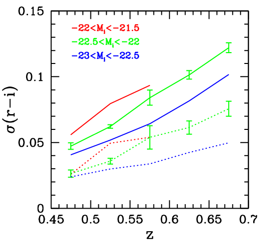
Examining Figures 5-7, there is a noticeable trend that the width of the red sequence appears narrower for more luminous galaxies and at lower redshifts. We highlight this effect in Figure 8, which presents the 1 width of the red sequence as a function of luminosity and redshift. Since the photometric errors become larger for fainter galaxies and at higher redshifts, we subtract their contribution in quadrature to obtain the intrinsic color width of the red sequence galaxies. The color photometric errors are estimated by simply combining in quadrature the errors in - and -band magnitudes (neglecting any additional errors in the k+e corrections and in the correlation between - and -band photometric errors). As shown in Figure 8, the above trend persists for the intrinsic color scatter, suggesting an evolutionary effect which we discuss further in Appendix A.
III.3.2 The Dependence of Galaxy 2PCF on Color

With the color cuts defined in the previous subsection, we investigate the dependence of galaxy 2PCFs on the color. First, we examine the 2PCFs for blue and red galaxies in the whole CMASS sample. The red and blue samples here are defined using the color cut in Equation 7. The samples are flux-limited (in addition to other selection cuts) and are by no means complete. The purpose of this exercise is simply to have an overall view of the difference in red and blue galaxy clustering. The measurements for blue and red galaxies are shown in Figure 9. For reference, the dotted circles in both panels are the angle-averaged redshift-space correlation function . Red galaxies are more strongly clustered. The “Fingers-of-God” feature [40] on small scales caused by random motions of galaxies in virialized structures can be clearly seen for both red and blue galaxies. Red galaxies have a stronger “Fingers-of-God” effect, reflecting their stronger motions within halos. On large scales (e.g., above , the outmost contours), the contours for both blue and red galaxies show the flattening trend caused by coherent large-scale infall [42]. On these scales, the Kaiser squashing effect appears to be stronger for blue galaxies, since the effect is determined by and blue galaxies have a smaller galaxy bias factor .

We now investigate the color-dependent 2PCFs as a function of luminosity and redshift from the fine color samples. In order to minimize the effect of incompleteness, the luminosity and redshift bins are selected using Figure 1 to make sure that red galaxies are not affected by the selection cuts. The blue galaxies are generally not complete at most redshifts and the results of the samples need to be interpreted with care. Nevertheless, the blue samples are still useful in comparison with the red galaxies.
The main results of the color-dependent 2PCFs are summarized in Figure 10. The top panels display the dependence of on color in the magnitude range at two different redshift intervals. The trend with color is obvious at both redshifts – there is a continuous increase in the clustering amplitude as galaxy color goes from blue to red. This result is consistent with the behavior observed in the SDSS-I/II main galaxy sample (Z11). On small scales (below the inflection scale of 1–2), there appears to be a trend that redder galaxies have a steeper slope in , which is weaker than that measured by Z11. According to the HOD modeling result in Z11, for galaxies in a fixed luminosity range, redder galaxies generally have a higher fraction of satellites residing in massive halos. Our results therefore implies that a larger fraction of redder galaxies reside in more massive halos, giving rise to a larger clustering amplitude. The steepening of on smaller scales may also indicate a halo mass scale shift with color, leading to a relative increase in the contribution from the 1-halo central-satellite pairs with respect to the 1-halo satellite-satellite pairs (see the Appendix A of Zheng et al. 113).
The bottom panels of Figure 10 present the 2PCFs for more luminous red galaxies, with , showing the results for the redseq and reddest color subsets. The number densities of these two subsets have a roughly constant value of and over the redshift range, respectively. There is a stronger inflection in the slope of below for these luminous galaxies and a trend of steeper slope for the reddest sample than for the redseq sample, indicating the shift in the halo mass scale. The two bottom panels also compare the redshift evolution for galaxies of the same color and luminosity. No strong evolution in is found, consistent with the bottom right panel of Figure 4. The implications of these results are discussed further in Section IV.
III.4. Red Galaxy Samples with Fixed Number Density

In previous sections, we constructed galaxy samples in certain luminosity and color bins, in an attempt to minimize the influence of incompleteness caused by target selection cuts. Motivated by a simple passive evolution model, we can further define galaxy samples with fixed number density at different redshifts [102, 10, 98]. If during the evolution each galaxy in a sample retains its identity, experiencing no merger or disruption, the number density of the galaxy sample would not change with redshift. The evolution of the 2PCF of such a galaxy sample can be readily predicted [30]. If, in addition, no star formation occurs in these galaxies during the process, their stellar population would evolve passively and can be readily modeled [98, 96]. Comparing to such predictions allows a rough determination of the extent of evolution in the red galaxy samples.
We construct three such samples for the red galaxies, which may be expected to resemble a passively evolving population, with fixed low, moderate and high number densities. For each sample, the fixed number density is achieved by finding a (redshift-dependent) luminosity threshold and selecting all galaxies with luminosity above this threshold, as shown in Figure 11. The luminosity and redshift ranges are chosen to reduce the sample incompleteness caused by the selection cuts. The low, moderate, and high number density samples have of , , and , respectively.
As seen in Figure 11, the fixed number density thresholds correspond globally to rough luminosity thresholds, decreasing with increasing number density as expected. The luminosity thresholds stay roughly constant for the red galaxies at . Since the luminosities in our study have been k+e corrected, this result implies that the stellar population in these red galaxies evolves passively. The drop below is likely caused by the incompleteness of galaxies at lower redshift due to the CMASS selection cuts, as discussed in Section II.2.

The projected 2PCFs for the fixed number density samples of red galaxies are presented in Figure 12. The top panels show that the clustering strength is inversely proportional to the number density, such that galaxies in the lower number density samples are more clustered. These results are generally consistent with the luminosity dependence discussed in Section III.2, as the different values of effectively act as different luminosity thresholds. The shapes of the 2PCFs for different samples are similar. The bottom panels compare the 2PCFs of the same samples at different redshift intervals. We find that the 2PCFs at different redshifts have similar clustering strength, again consistent with the results for the luminosity dependence of red galaxies (Figure 4, bottom-right panel). We discuss the implications of these results next.
III.5. Galaxy Bias
With the measured galaxy 2PCFs and the theoretical matter 2PCF for the cosmology adopted in this paper, we can infer the galaxy linear bias factor from the square root of the ratio between the galaxy and dark matter 2PCFs. The evolution of the linear bias factor can provide hints about the evolution of galaxy samples. In this subsection, we present the results on galaxy linear bias factor as a function of galaxy luminosity, color, number density, and redshift, and discuss the possible implications on galaxy evolution. Since blue galaxies in the CMASS sample are generally far from complete, we will focus our discussion on the bias evolution of the red galaxies.
At each redshift, for each galaxy sample, we estimate the linear bias factor by taking the square root of the ratio between the measured projected galaxy 2PCF and the non-linear dark matter projected 2PCF computed at the corresponding redshift, where the latter is calculated using a modified halofit model [88] with the Eisenstein & Hu [25] power spectrum parameterization. More specifically, we fit the ratio of galaxy and matter with a single parameter on scales , using the full covariance matrix of the galaxy .
Fry [30] shows that the passive evolution prediction for the linear bias factor follows
| (19) |
where is the linear growth factor at redshift and is the bias factor at (). From this relation, the redshift evolution of galaxy 2PCF for the passively-evolving population can be expressed as
| (20) |
where is the matter 2PCF at . Here we use the word “passive” to mean that during the evolution, each galaxy in the sample keeps its identity and there is no merger or disruption that changes the population. For the CMASS sample considered in this paper, the galaxy bias factor is usually greater than unity. Therefore, according to the above two equations, for passively-evolving galaxies, we expect that with decreasing redshift the amplitude of 2PCF increases while the bias factor decreases.

Figure 13 shows the bias redshift evolution for luminosity bin samples (left) and for the fixed number density samples (right). The bias factors are measured for non-overlapping redshift bins. The fitted bias factors support our results in the previous subsections that more luminous (or lower density) samples are more strongly clustered. The dotted lines in Figure 13 are the best-fit Fry [30] relation for each sample, with as the single fitting parameter. For the two luminosity-bin red galaxy samples, we find that they roughly follow the passive evolution prediction. Strictly speaking, each luminosity bin sample does not conserve the number density at different redshifts. So by definition it is not a passively-evolving population. However, these number density differences may be accounted for by slightly changing the luminosity thresholds of the luminosity bin sample at each redshift (e.g., as a result of an imperfect k+e correction). The measured bias would not be sensitive to such an adjustment. In such a sense, comparing their bias evolution to the Fry relation can still be meaningful.
For both the luminous and faint samples, there is suggestive evidence that the clustering at intermediate redshifts ( for the luminous sample, and for the faint sample) is slightly weaker than that from the best-fit passive evolution. Similar deviations from passive evolution were found in other works (e.g., White et al. 102, Wake et al. 98, Sawangwit et al. 77). However, the large measurement errors in our results make the deviation only at about level, limiting our ability for a solid conclusion.
If this deviation is robustly established, with more accurate future measurements using CMASS data over a larger survey area, it would imply a significant contribution from processes that break passive evolution, such as feedback from active galactic nuclei shutting off star formation, disruption of satellites in massive halos, and mergers of galaxies [4, 28, 84]. The signature may be related to the overall migration of blue galaxies to the red sequence [53], in which case, it would indicate appreciable migration by , consistent with the prediction of [28]. A sophisticated model is needed to disentangle the contributions from the different evolutionary processes.
The more reliable samples to study the passive evolution are the ones with fixed number densities, as described in Section III.4. The results for our three samples are shown in the right panel of Figure 13. The low sample appears consistent with passive evolution in the redshift range , within the (large) error bars on the measurements. This behavior is similar to the sample. In fact the low sample is close to a luminosity-threshold sample of , as shown in Figure 11. For the two samples with higher , their bias evolution is consistent with passive evolution for the smaller redshift ranges probed, which is in agreement with the conclusions of [96]. Within the current uncertainties, however, it is not possible to make strong statements regarding confirming or ruling out passive evolution. We will revisit this with more accurate measurements with future larger CMASS samples.

Finally, we present the dependence of the bias factor on luminosity in Figure 14 for all galaxies and for the red galaxies only. Generally, more luminous and redder galaxies at higher redshifts have larger bias factors. For the fainter samples, the bias factors are similar in the two cases, since at the faint end red galaxies dominate the CMASS sample (the majority of the faint blue galaxies are excluded by the selection cuts). The observed dependence of galaxy bias factor on galaxy luminosity is broadly similar to that for local galaxy samples (e.g., Norberg et al. 61, Z11), but it is non-trivial to compare in detail due to the many differences in sample selection, redshift, k+e corrections and magnitudes.
We fit the bias-luminosity relation with a commonly-used simple functional form [61, 110],
| (21) |
We define as the mean luminosity of galaxies in the faintest luminosity bin. This sample of galaxies has , so by construction, . We fit this functional form to the luminosity-dependent bias measurements at , finding for all galaxies and for the red galaxies (shown as the red dotted curves in Figure 14). At higher redshifts, , the bias factors for all galaxies show a decrease compared to the lower-redshift relation due to the inclusion of more blue galaxies at high redshifts. In contrast, the bias factors for the red galaxies globally increase with redshift, as expected from passive evolution. The dashed curve in the right panel shows the low-redshift relation shifted to high redshift according to the Fry relation prediction, which is in agreement with our measurements.
IV. Conclusion and Discussion
In this paper, we measure the luminosity and color dependence of the galaxy 2PCFs based on BOSS CMASS DR9 galaxies over a survey area in the redshift range of and study the implications on galaxy formation and evolution.
We first measure the 2PCF for the entire sample. If approximated by a power-law, the 2PCF has a correlation length of and a slope of , consistent with the measurements presented by White et al. [103] and Nuza et al. [63]. We also construct color and luminosity subsamples. To reduce the influence of sample incompleteness caused by the target selection criteria of CMASS galaxies, we carefully account for the selection cuts in the color-luminosity distribution of galaxies at each redshift interval in defining our subsamples. These subsamples in certain color and luminosity bins are close to complete and volume-limited. In order to compare the clustering of galaxy populations at different redshifts, we perform k+e correction to the magnitudes and colors of the galaxies using FSPS models. Such corrections are unavoidably dependent on the specific stellar evolution models used. However, as shown in Appendix A, our general results on the clustering analysis would not be significantly affected.
We find that for all redshift intervals probed, more luminous galaxies are more strongly clustered, consistent with previous studies for galaxies at different redshifts, such as SDSS-I/II main sample galaxies at [110, 111], SDSS LRG galaxies at [109], and DEEP2 galaxies at [15]. At each redshift, the large-scale galaxy bias factor of CMASS galaxies shows a linear dependence on galaxy luminosity, similar to that for lower redshift galaxies (Norberg et al. 62, Z11), but with different coefficients in the bias-luminosity relation. We divide galaxies globally into a blue and a red population. For each population, we find a similar clustering trend – an increasing clustering strength with luminosity. For blue galaxies, our results are in line with that of Z11 for SDSS galaxies. For red galaxies, Z11 find that both the most luminous and faintest galaxies exhibit stronger small-scale () clustering than the samples of intermediate luminosity, which can be explained as a large satellite fraction in the faintest sample and high mass of host halos for the most luminous sample. Because CMASS selects mostly luminous galaxies, we are not able to investigate the trend towards faint red galaxies, but for the luminous red galaxies, our results agree with that in Z11.
We further investigate the dependence of clustering on galaxy color, using finer color cuts. For fixed redshift and luminosity, we find that redder galaxies exhibit stronger clustering, similar to the trend found for the SDSS main galaxies [110, 111, 47]. Interestingly, such a trend exists even within the red sequence, consistent with the finding of Zehavi et al. [110], Zehavi et al. [111]. The trend is different from that of DEEP2 galaxies in Coil et al. [16], where no clear color dependence is seen across the red sequence. If this difference is caused by galaxy evolution, it implies that the color dependence in the red sequence emerges during the redshift range of . The emergence of the dependence may signal the contribution of substantial amounts of mergers and inflow of blue galaxies to the buildup of the red sequence.
We also construct subsamples of red galaxies with fixed number densities by applying redshift-dependent luminosity thresholds, and compare their clustering with the theoretical prediction of passively-evolving galaxies [30]. We find that the evolution of the large-scale galaxy bias factors for all the three CMASS subsamples considered in this paper are consistent with that from the Fry relation, within the relatively large uncertainties in the measured bias factors, which suggests that the red galaxies in the CMASS sample roughly follow passive evolution from to . In contrast, from HOD modeling of clustering of red galaxies in NDWFS [10], White et al. [102] found that passive evolution from to would predict too many satellite galaxies in high-mass halos and concluded that about one-third of these satellites must have experienced merging or disruption. The apparent discrepancy between our result and that in White et al. [102] can be explained by the difference in the number densities of galaxy samples. The NDWFS samples analyzed in [102] have a constant comoving number density of , about one order of magnitude higher than the ones we study here. Thus, their constant number density samples include fainter red galaxies (which have a larger contribution from satellite galaxies). In contrast, galaxies in our more luminous samples are predominantly luminous central galaxies that roughly follow passive evolution (but see also Wake et al. 98, Sawangwit et al. 77). These results seem to support a scenario in which mergers and disruption play an important role for the evolution of low-mass red galaxies.
Our investigation of the color-luminosity distribution at each redshift reveals two notable trends in the width of the red sequence. The red sequence becomes narrower towards the high-luminosity end, and it becomes narrower towards lower redshifts. Similar results are also seen in galaxies at both lower and higher redshifts [4, 85, 101, e.g.,]. The color scatter in the red sequence reflects the distribution of the ages of stellar population, dust extinction, and metallicity. At a given redshift, fainter galaxies show a more diverse distribution of these quantities, leading to a wider distribution in color. Passive evolution makes galaxies redder and largely reduces the color difference caused by the distribution of the ages of stellar population, leading to a narrower red sequence towards lower redshifts.
The inferences in this paper about the evolution of CMASS galaxies from the measured color and luminosity dependent clustering are still based on simple clustering models and interpretations. A further, natural step to interpret these results is to perform HOD modeling of our measurements, which will allow us to better study galaxy formation and evolution by incorporating knowledge about the dark matter halo formation and evolution. We expect that improved measurements from larger BOSS samples in the future and detailed HOD modeling will greatly advance our understanding of the evolution of massive galaxies.
Appendix A A. Different Stellar Evolution Models
In this paper, we correct for the k+e effects using the FSPS model, as mentioned in II.2. [96] compare the FSPS model and the stellar evolution model of Maraston & Strömbäck (2011; M11), and conclude that both models provide similar star formation histories with similar mass-weighted ages. [96] also compare the large-scale clustering using both models, and find that they produce consistent results. We show in Figure 15 the color-magnitude diagram obtained using the two different models at two redshift ranges. Contour lines for the FSPS model are shown in red and for the M11 model in blue. The green line is our proposed color cut (using the FSPS model). The two models predict similar k+e corrections for , but at higher redshifts the M11 model appears to produce more luminous and bluer galaxies. The overall shapes of the distributions for the two models, however, are quite similar. In particular, using alternatively the M11 model would not tilt the slope of the red sequence. Using the M11 model, the detailed color cuts would be changed accordingly but the clustering dependence on the luminosity and color are not expected to change.

From the CMD, it appears that CMASS galaxies have a tail of faint extremely-red galaxies, which is different from the properties of the SDSS main sample (see, e.g., Z11). This appearance, however, is partly caused by the selection cuts, which remove most of the faint blue galaxies. To clarify this effect, we show in Figure 15 the galaxies from the BOSS CMASS Sparse Sample, which includes fainter and bluer galaxies by extending the sliding cut (Equation 3) to
| (A1) |
[64]. These faint blue galaxies are sparsely sampled to yield approximately five objects per square degree. It is clear that the red sequence has more triangular distribution in CMASS, as a result of the increase in the width of the color distribution for fainter galaxies (Figure 8 and discussion thereof). A similar shape of the red sequence is also observed at higher redshifts [101, see e.g., Figure 1 of]. The narrow red sequence shown in Z11 is caused by the fact that their CMD is for the flux-limited main sample galaxies. Many fainter galaxies at higher redshifts are excluded by the faint flux limit. If shown for a volume-limited sample, the “triangle” shape of the red sequence is more apparent (see e.g., Figure 2 of Skibba & Sheth 85). Since this Sparse Sample does not have the same selection as other CMASS galaxies, we do not include it in our analysis, but these galaxies can be useful for studying evolution of blue galaxies that have smaller stellar masses.
Appendix B B. Jackknife Error Estimates
We use the jackknife resampling method to construct the error covariance matrices (Equation 12). In principle, it is preferable to derive covariance matrices from large numbers of realistic mock catalogs, each matching the observed galaxy properties, survey geometry, and selection functions. However, our tests below demonstrate that the jackknife error estimates perform quite well and are sufficient for our purposes. Moreover, it is a far more practical tool when working with many subsamples of different clustering properties. We do not currently have available mocks with suitable modeling of the galaxy luminosity function and with the correct galaxy distribution on small scales. The large set of mock catalogs used by [2] are constructed by populating dark matter halos in simulations with galaxies according to the HOD model fitted to the redshift-space 2PCF on large scales (). The measured large-scale 2PCFs of galaxies are reasonably reproduced in these mocks, while the small-scale 2PCFs are not matched [see 51, for details]. Although the small scale 2PCFs measured from these mocks generally deviates from the real data, the mocks can still be used to evaluate the validity of the jackknife method, and the appropriate number of jackknife subsamples to use.


In the left panel of Figure 16, we compare the fractional diagonal errors of from variations among 100 mock catalogs of [51] (solid curve) and those from applying the jackknife resampling method to the mocks with different number of jackknife samples (symbols with different colors). The jackknife error estimates show excellent consistency with those estimated from variations among mocks, especially for scales less than a few . Around , the jackknife method slightly overestimates the errors (by 15%). The jackknife errors also appear to be insensitive to the total number of jackknife samples used, with a general convergence for 100 or more jackknife samples. We have also checked the off-diagonal elements in the covariance matrices and find that the jackknife estimates are generally consistent with the variations-among-mocks estimates, although there are somewhat larger fluctuations of the jackknife estimates from mock to mock. All the results are consistent with those found and discussed in [110].
[60] have performed a comprehensive study of a variety of error estimators for dark matter correlation functions in -body simulations, comparing estimates such as jackknife and bootstrap to those derived from multiple independent catalogs. They find good agreement between jackknife and external estimates for the variance in on large scales, consistent with our results in Figure 16. However, [60] find that the jackknife method significantly overestimates the errors in on small scales (e.g., by 40% at ), while we do not see such a large difference in our results. It is worth noting that we differ in our implementation of the jackknife method. While [60] estimate the jackknife errors by dividing the simulation boxes into subvolumes, we divide the sample into jackknife subsamples of equal area with the same radial selection. Also, the mocks used in [60] have smaller volume than the ones used in this paper, which might lead to larger uncertainties in their error estimates. It is possible that the differences in applying the jackknife method and in the uncertainties can explain the apparent difference between our results and those of [60].
The right panel of Figure 16 shows the jackknife error estimates for the entire CMASS sample. It is encouraging that the overall shape and magnitude of the fractional errors from the real data are in good general agreement with those from the mocks, even though the mocks do not intend to match the small-scale clustering. Since we do not see significant variations in the error estimates with 100 or more jackknife samples, we choose jackknife samples for the error estimation in this paper. With an effective area of about for the CMASS DR9 sample, each excluded jackknife region then has an area of , corresponding to about , large enough for measuring the 2PCF in the range presented in this paper (). The normalized jackknife covariance matrix with samples, for of the whole CMASS sample, is shown in Figure 17. While the correlation coefficients for the off-diagonal elements on small scales () are mostly below , the errors of on large scales are highly correlated. Therefore, when fitting for scales larger than , the full covariance matrix, not just the diagonal elements, should be taken into account.
References
- [1] Ahn, S.-I. C. C. P., Alexandroff, R., Allende Prieto, C., & et al. 2012, ApJS, 203, 21
- [2] Anderson, L., Aubourg, E., Bailey, S., et al. 2012, MNRAS, 427, 3435
- [3] Baldry, I. K., Glazebrook, K., Brinkmann, J., et al. 2004, ApJ, 600, 681
- [4] Bell, E. F., Wolf, C., Meisenheimer, K., et al. 2004, ApJ, 608, 752
- [5] Benoist, C., Maurogordato, S., da Costa, L. N., Cappi, A., & Schaeffer, R. 1996, ApJ, 472, 452
- [6] Berlind, A. A., & Weinberg, D. H. 2002, ApJ, 575, 587
- [7] Berlind, A. A., Weinberg, D. H., Benson, A. J., Baugh, C. M., Cole, S., et al. 2003, ApJ, 593, 1
- [8] Blanton, M. R., Eisenstein, D., Hogg, D. W., Schlegel, D. J., & Brinkmann, J. 2005, ApJ, 629, 143
- [9] Bolton, A. S., Schlegel, D. J., Aubourg, E., et al. 2012, AJ, 144, 144
- [10] Brown, M. J. I., Zheng, Z., White, M., et al. 2008, ApJ, 682, 937
- [11] Budavári, T., Connolly, A. J., Szalay, A. S., et al. 2003, ApJ, 595, 59
- [12] Cannon, R., Drinkwater, M., Edge, A., et al. 2006, MNRAS, 372, 425
- [13] Chen, Y.-M., Kauffmann, G., Tremonti, C. A., et al. 2012, MNRAS, 421, 314
- [14] Christodoulou, L., Eminian, C., Loveday, J., et al. 2012, MNRAS, 425, 1527
- [15] Coil, A. L., Newman, J. A., Cooper, M. C., et al. 2006, ApJ, 644, 671
- [16] Coil, A. L., Newman, J. A., Croton, D., et al. 2008, ApJ, 672, 153
- [17] Conroy, C., & Gunn, J. E. 2010, ApJ, 712, 833
- [18] Conroy, C., Gunn, J. E., & White, M. 2009, ApJ, 699, 486
- [19] Conroy, C., Wechsler, R. H., & Kravtsov, A. V. 2006, ApJ, 647, 201
- [20] Cooray, A., & Sheth, R. 2002, Phys. Rep., 372, 1
- [21] Davis, M., & Geller, M. J. 1976, ApJ, 208, 13
- [22] Davis, M., Meiksin, A., Strauss, M. A., da Costa, L. N., & Yahil, A. 1988, ApJ, 333, L9
- [23] Davis, M., & Peebles, P. J. E. 1983, ApJ, 267, 465
- [24] Dawson, K. S., Schlegel, D. J., Ahn, C. P., et al. 2013, AJ, 145, 10
- [25] Eisenstein, D. J., & Hu, W. 1998, ApJ, 496, 605
- [26] Eisenstein, D. J., Annis, J., Gunn, J. E., et al. 2001, AJ, 122, 2267
- [27] Eisenstein, D. J., Weinberg, D. H., Agol, E., et al. 2011, AJ, 142, 72
- [28] Faber, S. M., Willmer, C. N. A., Wolf, C., et al. 2007, ApJ, 665, 265
- [29] Feldman, H. A., Kaiser, N., & Peacock, J. A. 1994, ApJ, 426, 23
- [30] Fry, J. N. 1996, ApJ, 461, L65
- [31] Fukugita, M., Ichikawa, T., Gunn, J. E., et al. 1996, AJ, 111, 1748
- [32] Gallazzi, A., Charlot, S., Brinchmann, J., & White, S. D. M. 2006, MNRAS, 370, 1106
- [33] Gunn, J. E., Carr, M., Rockosi, C., et al. 1998, AJ, 116, 3040
- [34] Gunn, J. E., Siegmund, W. A., Mannery, E. J., et al. 2006, AJ, 131, 2332
- [35] Guo, H., Zehavi, I., & Zheng, Z. 2012, ApJ, 756, 127
- [36] Guo, Q., White, S., Li, C., & Boylan-Kolchin, M. 2010, MNRAS, 404, 1111
- [37] Guzzo, L., Strauss, M. A., Fisher, K. B., Giovanelli, R., & Haynes, M. P. 1997, ApJ, 489, 37
- [38] Hamilton, A. J. S. 1988, ApJ, 331, L59
- [39] Hamilton, A. J. S. 1993, ApJ, 417, 19
- [40] Jackson, J. C. 1972, MNRAS, 156, 1P
- [41] Kaiser, N. 1984, ApJ, 284, L9
- [42] Kaiser, N. 1987, MNRAS, 227, 1
- [43] Kodama, T., & Arimoto, N. 1997, A&A, 320, 41
- [44] Komatsu, E., Smith, K. M., Dunkley, J., et al. 2011, ApJS, 192, 18
- [45] Kravtsov, A. V., Berlind, A. A., Wechsler, R. H., et al. 2004, ApJ, 609, 35
- [46] Landy, S. D., & Szalay, A. S. 1993, ApJ, 412, 64
- [47] Li, C., Kauffmann, G., Jing, Y. P., et al. 2006, MNRAS, 368, 21
- [48] Loh, Y.-S., Rich, R. M., Heinis, S., et al. 2010, MNRAS, 407, 55
- [49] Loveday, J., Maddox, S. J., Efstathiou, G., & Peterson, B. A. 1995, ApJ, 442, 457
- [50] Madgwick, D. S., Hawkins, E., Lahav, O., et al. 2003, MNRAS, 344, 847
- [51] Manera, M., Scoccimarro, R., Percival, W. J., et al. 2013, MNRAS, 428, 1036
- [52] Maraston, C., Pforr, J., Henriques, B. M., et al. 2012, MNRAS, in press, arXiv:1207.6114
- [53] Martin, D. C., Wyder, T. K., Schiminovich, D., et al. 2007, ApJS, 173, 342
- [54] Masters, K. L., Maraston, C., Nichol, R. C., et al. 2011, MNRAS, 418, 1055
- [55] Meneux, B., Le Fèvre, O., Guzzo, L., et al. 2006, A&A, 452, 387
- [56] Meneux, B., Guzzo, L., Garilli, B., et al. 2008, A&A, 478, 299
- [57] Meneux, B., Guzzo, L., de la Torre, S., et al. 2009, A&A, 505, 463
- [58] Mo, H. J., & White, S. D. M. 1996, MNRAS, 282, 347
- [59] Mostek, N., Coil, A. L., Cooper, M. C., et al. 2012, ApJ, submitted, arXiv:1210.6694
- [60] Norberg, P., Baugh, C. M., Gaztañaga, E., & Croton, D. J. 2009, MNRAS, 396, 19
- [61] Norberg, P., Baugh, C. M., Hawkins, E., et al. 2001, MNRAS, 328, 64
- [62] Norberg, P., Baugh, C. M., Hawkins, E., et al. 2002, MNRAS, 332, 827
- [63] Nuza, S. E., Sanchez, A. G., Prada, F., et al. 2012, MNRAS, submitted, arXiv:1202.6057
- [64] Padmanabhan, N., et al. 2013, in preparation
- [65] Parejko, J. K., Sunayama, T., Padmanabhan, N., et al. 2013, MNRAS, 429, 98
- [66] Peacock, J. A., & Smith, R. E. 2000, MNRAS, 318, 1144
- [67] Reid, B. A., Samushia, L., White, M., et al. 2012, MNRAS, 426, 2719
- [68] Ross, A. J., & Brunner, R. J. 2009, MNRAS, 399, 878
- [69] Ross, A. J., Ho, S., Cuesta, A. J., et al. 2011a, MNRAS, 417, 1350
- [70] Ross, A. J., Percival, W. J., & Brunner, R. J. 2010, MNRAS, 407, 420
- [71] Ross, A. J., Percival, W. J., Carnero, A., et al. 2013, MNRAS, 428, 1116
- [72] Ross, A. J., Percival, W. J., Sánchez, A. G., et al. 2012, MNRAS, 424, 564
- [73] Ross, A. J., Tojeiro, R., & Percival, W. J. 2011b, MNRAS, 413, 2078
- [74] Ross, N. P., da Ângela, J., Shanks, T., et al. 2007, MNRAS, 381, 573
- [75] Samushia, L., Reid, B. A., White, M., et al. 2013, MNRAS, 429, 1514
- [76] Sánchez, A. G., Scóccola, C. G., Ross, A. J., et al. 2012, MNRAS, 425, 415
- [77] Sawangwit, U., Shanks, T., Abdalla, F. B., et al. 2011, MNRAS, 416, 3033
- [78] Schlegel, D. J., Finkbeiner, D. P., & Davis, M. 1998, ApJ, 500, 525
- [79] Scoccimarro, R., Sheth, R. K., Hui, L., & Jain, B. 2001, ApJ, 546, 20
- [80] Scóccola, C. G., Sánchez, A. G., Rubiño Martin, J. A., et al. 2012, MNRAS, submitted, arXiv:1209.1394
- [81] Scoville, N., Abraham, R. G., Aussel, H., et al. 2007, ApJS, 172, 38
- [82] Seljak, U. 2000, MNRAS, 318, 203
- [83] Shen, Y., McBride, C. K., White, M., et al. 2012, ApJ, submitted, arXiv:1212.4526
- [84] Skelton, R. E., Bell, E. F., & Somerville, R. S. 2009, ApJ, 699, L9
- [85] Skibba, R. A., & Sheth, R. K. 2009, MNRAS, 392, 1080
- [86] Skibba, R. A., Bamford, S. P., Nichol, R. C., et al. 2009, MNRAS, 399, 966
- [87] Smee, S., Gunn, J. E., Uomoto, A., et al. 2012, AJ, submitted, arXiv:1208.2233
- [88] Smith, R. E., Peacock, J. A., Jenkins, A., et al. 2003, MNRAS, 341, 1311
- [89] Springel, V., White, S. D. M., Jenkins, A., et al. 2005, Nature, 435, 629
- [90] Strateva, I., Ivezić, v. Z., Knapp, G. R., et al. 2001, AJ, 122, 1861
- [91] Swanson, M. E. C., et al. 2013, in preparation
- [92] Swanson, M. E. C., Tegmark, M., Blanton, M., & Zehavi, I. 2008, MNRAS, 385, 1635
- [93] Tinker, J. L., & Wetzel, A. R. 2010, ApJ, 719, 88
- [94] Tojeiro, R., Percival, W. J., Heavens, A. F., & Jimenez, R. 2011, MNRAS, 413, 434
- [95] Tojeiro, R., Percival, W. J., Brinkmann, J., et al. 2012a, MNRAS, 424, 2339
- [96] Tojeiro, R., Percival, W. J., Wake, D. A., et al. 2012b, MNRAS, 424, 136
- [97] Wang, Y., Yang, X., Mo, H. J., & van den Bosch, F. C. 2007, ApJ, 664, 608
- [98] Wake, D. A., Sheth, R. K., Nichol, R. C., et al. 2008, MNRAS, 387, 1045
- [99] Wake, D. A., Whitaker, K. E., Labbé, I., et al. 2011, ApJ, 728, 46
- [100] Weinberg, D. H., Mortonson, M. J., Eisenstein, D. J., et al. 2012, arXiv:1201.2434
- [101] Whitaker, K. E., van Dokkum, P. G., Brammer, G., et al. 2010, ApJ, 719, 1715
- [102] White, M., Zheng, Z., Brown, M. J. I., Dey, A., & Jannuzi, B. T. 2007, ApJ, 655, L69
- [103] White, M., Blanton, M., Bolton, A., et al. 2011, ApJ, 728, 126
- [104] Yang, X., Mo, H. J., Jing, Y. P., & van den Bosch, F. C. 2005, MNRAS, 358, 217
- [105] Yang, X., Mo, H. J., & van den Bosch, F. C. 2003, MNRAS, 339, 1057
- [106] York, D. G., Adelman, J., Anderson, Jr., J. E., et al. 2000, AJ, 120, 1579
- [107] Zehavi, I., Blanton, M. R., Frieman, J. A., et al. 2002, ApJ, 571, 172
- [108] Zehavi, I., Weinberg, D. H., Zheng, Z., et al. 2004, ApJ, 608, 16
- [109] Zehavi, I., Eisenstein, D. J., Nichol, R. C., et al. 2005a, ApJ, 621, 22
- [110] Zehavi, I., Zheng, Z., Weinberg, D. H., et al. 2005b, ApJ, 630, 1
- [111] Zehavi, I., Zheng, Z., Weinberg, D. H., et al. 2011, ApJ, 736, 59 [Z11]
- [112] Zheng, Z., Coil, A. L., & Zehavi, I. 2007, ApJ, 667, 760
- [113] Zheng, Z., Zehavi, I., Eisenstein, D. J., Weinberg, D. H., & Jing, Y. P. 2009, ApJ, 707, 554
- [114] Zheng, Z., Berlind, A. A., Weinberg, D. H., et al. 2005, ApJ, 633, 791