跳到论文正文
W Papers独立论文阅读器 arXiv:1212.1137 论文正文 计算阅读时间 · 0%
引用这篇论文根据当前论文元数据生成,正式投稿前建议核对。


License: arXiv.org perpetual non-exclusive license
arXiv:1212.1137v1 [math.NA] 05 Dec 2012

Discrete Total Variation Flows Without RegularizationThanks: RHN and AJS are partially supported by NSF grants DMS-0807811 and DMS-1109325. AJS is also partially supported by NSF grant DMS-1008058 and an AMS-Simons grant.

Sören Bartels ††thanks: Abteilung für Angewandte Mathematik, Albert-Ludwigs-Universität Freiburg Hermann-Herder-Str.˜10 79104 Freiburg i.Br., Germany. bartels@mathematik.uni-freiburg.de    Ricardo H. Nochetto ††thanks: Department of Mathematics and Institute for Physical Science and Technology, University of Maryland, College Park, MD 20742, USA. rhn@math.umd.edu    Abner J. Salgado ††thanks: Department of Mathematics, University of Maryland, College Park, MD 20742, USA. abnersg@math.umd.edu
Abstract

We propose and analyze an algorithm for the solution of the L2L^{2}-subgradient flow of the total variation functional. The algorithm involves no regularization, thus the numerical solution preserves the main features that motivate practitioners to consider this type of energy. We propose an iterative scheme for the solution of the arising problems, show that the iterations converge, and develop a stopping criterion for them. We present numerical experiments which illustrate the power of the method, explore the solution behavior, and compare with regularized flows.

keywords
Total Variation; Singular Diffusion; Maximal Monotone Operators; Subgradient Flows; Variational Inequalities.
AMS
65N12; 65M60; 65N15; 65N30; 35K86; 35R35; 35R37; 65K15.

Draft Version of August 24, 2026, \currenttime.

1 Introduction

This work is concerned with the approximation of solutions to the following (formal) initial boundary value problem:

{ut=∇⋅(∇u|∇u|),in ​Ω×(0,T),∇u|∇u|⋅𝐧=0,on ​∂Ω,u|t=0=u0, in ​Ω.\begin{cases}\textup{{u}}_{t}=\nabla\!{\cdot}\left(\frac{\nabla\textup{{u}}}{\left|\nabla\textup{{u}}\right|}\right),&\text{in }\Omega\times(0,T),\\ \frac{\nabla\textup{{u}}}{\left|\nabla\textup{{u}}\right|}{\cdot}{\bf n}=0,\ \text{on }\partial\Omega,&\textup{{u}}|_{t=0}=\textup{{u}}_{0},\ \text{ in }\Omega.\end{cases} (1.1)

Here Ω\Omega is an open, bounded and connected subset of ℝd\mathbb{R}^{d} with d≥1d\geq 1; ∂Ω\partial\Omega denotes the boundary of Ω\Omega and 𝐧{\bf n} its exterior unit normal; and T>0T>0 is a positive and finite time. This equation and related ones are commonly known as very singular diffusion equations (see [26, 27]) since in flat regions, i.e., |∇u|=0|\nabla\textup{{u}}|=0, the diffusion is so strong that it is not a local effect anymore.

Beginning with the seminal paper [34] equations of this class have received considerable attention from the image processing community, since such models preserve discontinuities while removing noise and other artifacts (see also [11, 13, 16, 17, 31]). In addition, such equations appear in the modeling of grain boundary motion [29]; facet formation and evolution [23]; electromigration [25] and various other problems stemming from materials science. This clearly shows that the development of efficient and accurate numerical schemes for the solution of this class of problems is of extreme importance. To the best of our knowledge however, the techniques advocated in the literature for the solution of these equations as a rule involve a regularization somewhat related with replacing the singular term by

|∇u|ϵ=ϵ2+|∇u|2,ϵ>0;|\nabla\textup{{u}}|_{\epsilon}=\sqrt{\epsilon^{2}+|\nabla\textup{{u}}|^{2}},\quad\epsilon>0; (1.2)

see, for instance, [9, 19, 21, 22, 30]. The disadvantages of this approach are twofold: first, although these methods have been shown to converge, there is no clear understanding of the relation between the regularization parameter ϵ\epsilon and the discretization parameters; second, the regularization destroys certain fundamental features of the solutions which motivate the introduction of such models in the first place.

A notable exception to the trend mentioned above is the work [7] which, inspired by the ideas advanced in [12], develops a finite element scheme for total variation minimization which involves no regularization. In this work we adapt and extend the ideas presented in [7] to the study of total variation flows. We propose and analyze an unconditionally stable and convergent discretization scheme for the approximation of (1.1). In addition, we study an iterative scheme for the solution of the discrete problems and develop an a posteriori error estimator that provides a robust stopping criterion for the iterative scheme that guarantees that, although we only have approximate solutions, the convergence properties of the method are not affected.

This work is organized as follows. The notation and conventions are set in Section 2. In §2.1 we recall the definition and main properties of functions of bounded variation and, in addition, we present an approximation result for these functions. This will be our workhorse during the derivation of error estimates. The proper framework to understand (1.1), i.e., total variation flow and its properties are described in Section 3. Time and space discretization are discussed in Section 4, where we begin by reviewing results on implicit semidiscretizations of gradient flows in Hilbert spaces. Then we provide a general theory for fully discrete subgradient flows in Hilbert spaces, which we later apply to our problem. One of the salient novelties of this general theory is that we allow for modifications in the energy which can be used, for instance, to take into account the effects of quadrature. In Section 5 we propose an iterative scheme for the solution of the fully discrete problems, and devise a stopping criterion for the iterations, which guarantees that the convergence orders are not damaged. Section 6 contains a series of numerical experiments, which illustrate and extend the properties and theory for the developed scheme. Finally, in Section 7, we apply the approximation result of §2.1 to the problem of total variation minimization and prove convergence estimates similar to those available in the literature, but with reduced regularity assumptions.

2 Notation and Preliminaries

We denote by Ω\Omega a bounded domain in ℝd\mathbb{R}^{d} with d≥1d\geq 1. The boundary of Ω\Omega is denoted by ∂Ω\partial\Omega and we assume that ∂Ω∈𝒞0,1\partial\Omega\in{\mathcal{C}}^{0,1}. We set T>0T>0 to be a finite final time. As usual, we denote by Lp​(Ω)L^{p}(\Omega) the space of Lebesgue integrable functions with exponent p∈[1,∞]p\in[1,\infty] and by Wps​(Ω)W^{s}_{p}(\Omega), s∈ℝs\in\mathbb{R}, the usual Sobolev spaces. Spaces of vector valued functions and their elements will be represented with boldface characters. Recall that the following interpolation inequality holds (cf. [24])

‖w‖Lr≤‖w‖Lps​‖w‖Lq1−s,p,q∈[1,∞],1r=sp+1−sq,s∈[0,1].\|w\|_{L^{r}}\leq\|w\|_{L^{p}}^{s}\|w\|_{L^{q}}^{1-s},\quad p,q\in[1,\infty],\ \frac{1}{r}=\frac{s}{p}+\frac{1-s}{q},\ s\in[0,1]. (2.1)

Whenever EE is a normed space, we denote its norm by ∥⋅∥E\|\cdot\|_{E} and its dual by E′E^{\prime}. The L2L^{2}-inner product will be denoted by ⟨⋅,⋅⟩\left\langle\cdot,\cdot\right\rangle. Function spaces of vector-valued functions will be denoted by boldface characters. For function spaces, if it is clear from the context, we will omit the domain of definition. We denote by 𝔅1​(E){\mathfrak{B}}_{1}(E) the unit ball in EE, i.e., the set 𝔅1​(E)={x∈E:‖x‖E≤1}.{\mathfrak{B}}_{1}(E)=\left\{x\in E:\|x\|_{E}\leq 1\right\}. Let ϕ:[0,T]→E\phi:[0,T]\rightarrow E be a measurable function in the Bochner sense, then, for p∈[1,∞]p\in[1,\infty], we define

‖ϕ‖Lp​(E)p=∫0T‖ϕ⁡(t)‖Ep​d​t,p<∞,‖ϕ‖L∞​(E)=ess​supt∈[0,T]⁡‖ϕ⁡(t)‖E.\|\phi\|_{L^{p}(E)}^{p}=\int_{0}^{T}\|\phi(t)\|_{E}^{p}\,\mbox{\rm d}t,\ p<\infty,\qquad\|\phi\|_{L^{\infty}(E)}=\esssup_{t\in[0,T]}\|\phi(t)\|_{E}.

We will denote by d​ϕd​t\tfrac{\,\mbox{\rm d}\phi}{\,\mbox{\rm d}t} the time derivative of ϕ\phi.

To deal with time discretization, we introduce a time-step Δ​t>0{\Delta t}>0, for simplicity assumed constant. Then we partition the time interval via tk=k​Δ​tt^{k}=k{\Delta t} with k=0,K¯k=\overline{0,K} and K=⌈T/Δ​t⌉K=\lceil T/{\Delta t}\rceil. We use the notation ϕΔ​t={ϕk}k=0K\phi^{\Delta t}=\left\{\phi^{k}\right\}_{k=0}^{K}, introduce the time increment operator

δ​ϕk=ϕk−ϕk−1,{\delta}\phi^{k}=\phi^{k}-\phi^{k-1}, (2.2)

and the extrapolation operator

ϕ⋆,k+1=ϕ0,k=0,ϕ⋆,k+1=ϕk+δ​ϕk,k>0.\phi^{\star,k+1}=\phi^{0},\ k=0,\qquad\phi^{\star,k+1}=\phi^{k}+{\delta}\phi^{k},\ k>0. (2.3)

For ϕΔ​t⊂E\phi^{\Delta t}\subset E and p∈[1,∞]p\in[1,\infty], we introduce the (semi)norms

‖ϕΔ​t‖ℓp​(E)p=Δ​t​∑k=0K‖ϕk‖Ep,‖ϕΔ​t‖𝔥1/2​(E)2=∑k=1K‖δ​ϕk‖E2,\|\phi^{\Delta t}\|_{\ell^{p}(E)}^{p}={\Delta t}\sum_{k=0}^{K}\|\phi^{k}\|_{E}^{p},\quad\|\phi^{\Delta t}\|_{{\mathfrak{h}}^{1/2}(E)}^{2}=\sum_{k=1}^{K}\|{\delta}\phi^{k}\|_{E}^{2},

with the usual modification for p=∞p=\infty. Given a sequence ϕΔ​t⊂E\phi^{\Delta t}\subset E we will want to be able to compare it to functions defined on [0,T][0,T]. To this end, we define the Rothe interpolant ϕ^\widehat{\phi}, that is, the piecewise linear function

ϕ^​(t)=t−tkΔ​t​ϕk+1+tk+1−tΔ​t​ϕk,t∈[tk,tk+1].\widehat{\phi}(t)=\frac{t-t^{k}}{{\Delta t}}\phi^{k+1}+\frac{t^{k+1}-t}{{\Delta t}}\phi^{k},\quad t\in[t^{k},t^{k+1}]. (2.4)

Notice that, by construction, ϕ^∈𝒞0,1​(E)\widehat{\phi}\in{\mathcal{C}}^{0,1}(E), and ‖ϕ^‖L∞​(E)=‖ϕΔ​t‖ℓ∞​(E)\|\widehat{\phi}\|_{L^{\infty}(E)}=\|\phi^{\Delta t}\|_{\ell^{\infty}(E)}. Recall also the well-known summation by parts formula: for every ϕΔ​t,ψΔ​t⊂L2​(Ω)\phi^{\Delta t},\psi^{\Delta t}\subset{{L}^{2}(\Omega)},

∑k=0K−1(⟨ϕk,δ​ψk+1⟩+⟨δ​ϕk+1,ψk+1⟩)=⟨ϕK,ψK⟩−⟨ϕ0,ψ0⟩.\sum_{k=0}^{K-1}\left(\left\langle\phi^{k},{\delta}\psi^{k+1}\right\rangle+\left\langle{\delta}\phi^{k+1},\psi^{k+1}\right\rangle\right)=\left\langle\phi^{K},\psi^{K}\right\rangle-\left\langle\phi^{0},\psi^{0}\right\rangle. (2.5)

We will carry out the space discretization with finite element techniques. In other words, given Ω\Omega we introduce a so-called triangulation 𝒯h={T}{\mathcal{T}}_{h}=\{T\} as a collection of cells that satisfy the usual conformity and shape regularity assumptions [14, 20], and are such that Ω¯=⋃T∈𝒯hT¯\bar{\Omega}=\bigcup_{T\in{\mathcal{T}}_{h}}\bar{T}. We parametrize our collection of triangulations via h=max⁡{diam⁡(T):T∈𝒯h}h=\max\left\{\diam(T):T\in{\mathcal{T}}_{h}\right\}. For simplicity, we assume that each TT is the isoparametric image of a so-called reference cell, which can be either T^=[−1,1]d\widehat{T}=[-1,1]^{d}, in which case we call the cells cubic; or T^={(x1,…,xd)∈ℝd:xi≥0​∑i=1dxi≤1},\widehat{T}=\left\{(x_{1},\ldots,x_{d})\in\mathbb{R}^{d}:\ x_{i}\geq 0\ \sum_{i=1}^{d}x_{i}\leq 1\right\}, which are called simplices. We denote by {zj,T}\{z_{j,T}\} the vertices of the cell TT and set 𝒩T=#⁡{zj,T}{\mathcal{N}}_{T}=\#\{z_{j,T}\}. Clearly, 𝒩T=2d{\mathcal{N}}_{T}=2^{d} for cubes and 𝒩T=d+1{\mathcal{N}}_{T}=d+1 for simplices.

We define the finite element space

𝕍h={wh∈𝒞0​(Ω¯):vh|T∈𝒫}⊂W∞1​(Ω),{\mathbb{V}}_{h}=\left\{w_{h}\in{\mathcal{C}}^{0}(\bar{\Omega}):v_{h}|_{T}\in{\mathcal{P}}\right\}\subset W^{1}_{\infty}(\Omega), (2.6)

where 𝒫=ℚ1{\mathcal{P}}={\mathbb{Q}}_{1} for cubes and 𝒫=ℙ1{\mathcal{P}}={\mathbb{P}}_{1} for simplices. Here ℚ1{\mathbb{Q}}_{1} denotes the space of polynomials of degree at most one in each variable and ℙ1{\mathbb{P}}_{1} the space of polynomials of total degree not greater than one.

For a function ww such that w|T∈𝒞0​(T¯)w|_{T}\in{\mathcal{C}}^{0}(\bar{T}), we define its local Lagrange interpolant ℐh​w{\mathcal{I}}_{h}w by

ℐh​w|T∈𝒫:ℐh​w|T​(zj,T)=w|T​(zj,T),j=1,𝒩T¯,∀T∈𝒯h.{\mathcal{I}}_{h}w|_{T}\in{\mathcal{P}}:\ {\mathcal{I}}_{h}w|_{T}(z_{j,T})=w|_{T}(z_{j,T}),\quad j=\overline{1,{\mathcal{N}}_{T}},\quad\forall T\in{\mathcal{T}}_{h}. (2.7)

This operator satisfies

‖w−ℐh​w‖Lp​(T)+h​‖∇(w−ℐh​w)‖Lp​(T)≤c​h2​‖D2​w‖Lp​(T),\|w-{\mathcal{I}}_{h}w\|_{L^{p}(T)}+h\|\nabla(w-{\mathcal{I}}_{h}w)\|_{L^{p}(T)}\leq ch^{2}\|D^{2}w\|_{L^{p}(T)}, (2.8)

see, e.g. [14], for a proof. We remark also that if w∈𝒞0​(Ω¯)w\in{\mathcal{C}}^{0}(\bar{\Omega}), then ℐh​w∈𝕍h{\mathcal{I}}_{h}w\in{\mathbb{V}}_{h}. It will be also necessary to introduce the Clément interpolant (cf. [15]) Πh:L1​(Ω)→𝕍h\Pi_{h}:L^{1}(\Omega)\rightarrow{\mathbb{V}}_{h}. This operator enjoys approximation properties similar to (2.8), the only difference being that the domain on the right hand side is a neighborhood of TT. More importantly, the operator is stable under any Sobolev norm, i.e.,

‖Πh​w‖Wps≤c​‖w‖Wps,s≥0,p∈[1,∞].\|\Pi_{h}w\|_{W^{s}_{p}}\leq c\|w\|_{W^{s}_{p}},\quad s\geq 0,\ p\in[1,\infty]. (2.9)

We will denote by cc a constant whose value might change at each occurrence.

2.1 Functions of Bounded Variation and their Approximation

We say that a function w∈L1​(Ω)w\in L^{1}(\Omega) belongs to the space B​V​(Ω)BV(\Omega) (is of bounded variation) if its derivative, D​w{\textup{D}}w, in the sense of distributions is a Radon measure. In other words, |D​w|​(Ω)<∞|{\textup{D}}w|(\Omega)<\infty, where for any Borel set A⊂Ω,A\subset\Omega,

|Dw|(A)=sup{∫Aw∇⋅𝐪:𝐪∈𝒞0∞(A),∥𝐪∥𝐋∞​(A)≤1}.|{\textup{D}}w|(A)=\sup\left\{\int_{A}w\nabla\!{\cdot}{\bf q}:\ {\bf q}\in{\mathcal{C}}_{0}^{\infty}(A),\,\|{\bf q}\|_{{\bf L}^{\infty}(A)}\leq 1\right\}.

The space B​V​(Ω)BV(\Omega) endowed with the norm ‖w‖B​V=‖w‖L1+|D​w|(Ω)\|w\|_{BV}=\|w\|_{L^{1}}+|{\textup{D}}w|(\Omega) is a Banach space. For more details on this space, we refer to [1, 38]. Let us present a result on approximation by smooth functions, in the case of a star-shaped domain.

Proposition 2.1 (Approximation of B​VBV functions).

Assume that Ω\Omega is bounded, star-shaped with respect to a point and ∂Ω∈𝒞0,1\partial\Omega\in{\mathcal{C}}^{0,1}. If w∈B​V​(Ω)w\in BV(\Omega), then for every ϵ>0\epsilon>0 there exists a wϵ∈𝒞∞​(Ω)w_{\epsilon}\in{\mathcal{C}}^{\infty}(\Omega) such that

‖w−wϵ‖L1≤ϵ​|D​w|​(Ω),‖∇wϵ‖L1≤(1+c​ϵ)​|D​w|​(Ω),‖D2​wϵ‖L1≤c​ϵ−1​|D​w|​(Ω).\|w-w_{\epsilon}\|_{L^{1}}\leq\epsilon|{\textup{D}}w|(\Omega),\quad\|\nabla w_{\epsilon}\|_{L^{1}}\leq(1+c\epsilon)|{\textup{D}}w|(\Omega),\quad\|D^{2}w_{\epsilon}\|_{L^{1}}\leq c\epsilon^{-1}|{\textup{D}}w|(\Omega).
Proof.

Without loss of generality, we can assume that 0∈Ω0\in\Omega and that Ω\Omega is star-shaped with respect to 00. For ϵ>0\epsilon>0 we define

Ωϵ={y∈ℝd:y=(1+ϵ)x,x∈Ω},\Omega_{\epsilon}=\left\{y\in\mathbb{R}^{d}:y=(1+\epsilon)x,\ x\in\Omega\right\},

and notice that Ω\Omega and Ωϵ\Omega_{\epsilon} are related via a bijective and Lipschitz, in fact linear, transformation with Lipschitz constant 1+ϵ1+\epsilon and Jacobian (1+ϵ)d≤1+c​ϵ(1+\epsilon)^{d}\leq 1+c\epsilon. For w∈B​V​(Ω)w\in BV(\Omega) we define vϵ∈B​V​(Ωϵ)v_{\epsilon}\in BV(\Omega_{\epsilon}) via vϵ​(y)=w​(y1+ϵ)v_{\epsilon}(y)=w(\tfrac{y}{1+\epsilon}) and, for x∈Ωx\in\Omega, wϵ​(x)=vϵ∗ρϵ​(x)w_{\epsilon}(x)=v_{\epsilon}*\rho_{\epsilon}(x), where ρϵ\rho_{\epsilon} is a smooth convolution kernel such that, for ever 1≤p≤∞1\leq p\leq\infty, ‖∇ρϵ‖Lp≤c​ϵ−(1+d/p′)\|\nabla\rho_{\epsilon}\|_{L^{p}}\leq c\epsilon^{-(1+d/p^{\prime})} with p′=p/(p−1)p^{\prime}=p/(p-1).

If w∈𝒞1​(Ω)w\in{\mathcal{C}}^{1}(\Omega) then, clearly, ‖w−wϵ‖L1<ϵ​‖∇w‖L1=ϵ​|D​w|​(Ω)\|w-w_{\epsilon}\|_{L^{1}}<\epsilon\|\nabla w\|_{L^{1}}=\epsilon|{\textup{D}}w|(\Omega) and

‖∇wϵ‖L1≤|D​vϵ|(Ωϵ)≤(1+c​ϵ)​‖∇w‖L1=(1+c​ϵ)​|D​w|​(Ω).\|\nabla w_{\epsilon}\|_{L^{1}}\leq|{\textup{D}}v_{\epsilon}|(\Omega_{\epsilon})\leq(1+c\epsilon)\|\nabla w\|_{L^{1}}=(1+c\epsilon)|{\textup{D}}w|(\Omega).

We now recall that smooth functions are dense in B​V​(Ω)BV(\Omega) under strict convergence, (cf. [1, 38]). In other words, given w∈B​V​(Ω)w\in BV(\Omega) there is a sequence {wn}n∈ℕ⊂𝒞∞​(Ω)\{w_{n}\}_{n\in{\mathbb{N}}}\subset{\mathcal{C}}^{\infty}(\Omega) such that

limn→∞‖w−wn‖L1=0,lim supn→∞|D​wn|​(Ω)≤|D​w|​(Ω).\lim_{n\rightarrow\infty}\|w-w_{n}\|_{L^{1}}=0,\qquad\limsup_{n\rightarrow\infty}|{\textup{D}}w_{n}|(\Omega)\leq|{\textup{D}}w|(\Omega).

Applying the argument given above to elements of this sequence and then passing to the limit we obtain the first two inequalities.

We use Young’s inequality for convolutions [24, Proposition 8.7] to obtain

‖D2​wϵ‖L1≤‖∇wϵ‖L1​‖∇ρϵ‖L1≤c​1+c​ϵϵ​|D​w|​(Ω)≤cϵ​|D​w|​(Ω),\|D^{2}w_{\epsilon}\|_{L^{1}}\leq\|\nabla w_{\epsilon}\|_{L^{1}}\|\nabla\rho_{\epsilon}\|_{L^{1}}\leq c\frac{1+c\epsilon}{\epsilon}|{\textup{D}}w|(\Omega)\leq\frac{c}{\epsilon}|{\textup{D}}w|(\Omega),

which concludes the proof. ∎

Remark 2.2 (Approximation in LpL^{p}-spaces).

Observe that, in the setting of Proposition 2.1, Young’s inequality also implies

‖D2​wϵ‖Lp≤‖∇wϵ‖L1​‖∇ρϵ‖Lp≤c​ϵ−(1+d/p′)​|D​w|​(Ω),\|D^{2}w_{\epsilon}\|_{L^{p}}\leq\|\nabla w_{\epsilon}\|_{L^{1}}\|\nabla\rho_{\epsilon}\|_{L^{p}}\leq c\epsilon^{-(1+d/p^{\prime})}|{\textup{D}}w|(\Omega),

for any p∈[1,∞]p\in[1,\infty] with p′=p/(p−1)p^{\prime}=p/(p-1). In the sequel, however, we shall avoid using this bound since it would lead to dd-dependent error estimates.

3 The Total Variation Flow

Let us define the functional Ψ:L2​(Ω)→ℝ\Psi:{{L}^{2}(\Omega)}\rightarrow\mathbb{R} by

Ψ⁡(w)={|D​w|​(Ω),w∈L2​(Ω)∩B​V​(Ω),+∞,w∈L2​(Ω)∖B​V​(Ω),\Psi(w)=\begin{cases}|{\textup{D}}w|(\Omega),&w\in{{L}^{2}(\Omega)}\cap BV(\Omega),\\ +\infty,&w\in{{L}^{2}(\Omega)}\setminus BV(\Omega),\end{cases} (3.1)

It is not difficult to show that Ψ\Psi is convex and lower semicontinuous. Then, one can define the subdifferential of Ψ\Psi (see [2, 6, 8, 10, 18, 26, 27]) and study its subgradient flow, i.e., we seek for a function u:[0,T]→L2​(Ω)\textup{{u}}:[0,T]\rightarrow{{L}^{2}(\Omega)} such that

ut∈−∂Ψ(u),\textup{{u}}_{t}\in-\partial\Psi(\textup{{u}}), (3.2)

or, equivalently,

⟨ut,u−w⟩+Ψ⁡(u)−Ψ⁡(w)≤0,∀w∈L2​(Ω).\left\langle\textup{{u}}_{t},\textup{{u}}-w\right\rangle+\Psi(\textup{{u}})-\Psi(w)\leq 0,\quad\forall w\in{{L}^{2}(\Omega)}. (3.3)

It is in this sense that (1.1) is going to be understood and analyzed. Existence of solutions to (3.2) can be obtained with the help of the theory of maximal monotone operators, see [6, 10].

Remark 3.1 (Dirichlet boundary conditions).

The definition that we have provided corresponds to imposing Neumann boundary conditions as in (1.1). The issue of how to impose Dirichlet boundary conditions is a delicate one since the trace of a B​V​(Ω)BV(\Omega) function is in L1​(∂Ω)L^{1}(\partial\Omega) (cf. [1, 38]). In addition, the functional (3.1) has linear growth, so that the only possible way to impose Dirichlet boundary conditions is with the relaxed energy Ψ⁡(w)+∫∂Ω|w−g|\Psi(w)+\int_{\partial\Omega}|w-g|; see [2, 28] for details. The introduction of this additional non-differentiable term greatly complicates the analysis. However, in the particular situation when Ω\Omega is convex, the boundary data is time independent and continuous, i.e., g⁡(x,t)=g⁡(x)∈𝒞0​(∂Ω)g(x,t)=g(x)\in{\mathcal{C}}^{0}(\partial\Omega), and the initial data is compatible with the boundary data in the sense that u0|∂Ω=g\textup{{u}}_{0}|_{\partial\Omega}=g, then the solution u to the subgradient flow with the relaxed energy satisfies u​(⋅,t)|∂Ω=g⁡(⋅)\textup{{u}}(\cdot,t)|_{\partial\Omega}=g(\cdot), for all t∈(0,T]t\in(0,T]; see [28, Lemma 4.1]. This can be realized, for instance, in the case of homogeneous Dirichlet boundary conditions (g≡0g\equiv 0) and compactly supported initial data. Under this particular setting all the results we present will also hold.

Reference [2, Theorem 2.16] shows that problem (3.2) possesses a LdL^{d}–L∞L^{\infty} regularizing effect, that is if u0∈Ld​(Ω)\textup{{u}}_{0}\in L^{d}(\Omega), then u​(t)∈L∞​(Ω)\textup{{u}}(t)\in L^{\infty}(\Omega) for all t>0t>0. Let us show that solutions to this problem also satisfy a maximum principle.

Theorem 3.2 (Maximum principle for TV flow).

Assume that u0∈L∞​(Ω)\textup{{u}}_{0}\in L^{\infty}(\Omega), then u, solution of (3.3), is such that u∈L∞​([0,T],L∞​(Ω))\textup{{u}}\in L^{\infty}([0,T],L^{\infty}(\Omega)) and

‖u‖L∞​(L∞)≤‖u0‖L∞.\|\textup{{u}}\|_{L^{\infty}(L^{\infty})}\leq\|\textup{{u}}_{0}\|_{L^{\infty}}.
Proof.

Since u0∈L∞​(Ω)\textup{{u}}_{0}\in L^{\infty}(\Omega) we can define 𝒰0=ess​supx∈Ω⁡u0​(x){\mathcal{U}}_{0}=\esssup_{x\in\Omega}\textup{{u}}_{0}(x), and w¯​(t)=u​(t)∨𝒰0\bar{w}(t)=\textup{{u}}(t)\vee{\mathcal{U}}_{0}. Since suppD​w¯={x∈Ω:u≥𝒰0}\mathop{\operator@font supp}\nolimits{\textup{D}}\bar{w}=\{x\in\Omega:\ \textup{{u}}\geq{\mathcal{U}}_{0}\} and, on this set, D​w¯=Du{\textup{D}}\bar{w}={\textup{D}}\textup{{u}}, we can conclude that w¯∈L2​(Ω)∩B​V​(Ω)\bar{w}\in{{L}^{2}(\Omega)}\cap BV(\Omega) and Ψ⁡(w¯)≤Ψ⁡(u)\Psi(\bar{w})\leq\Psi(\textup{{u}}). Setting w=w¯w=\bar{w} in (3.3) we obtain ⟨ut,0∨(u−𝒰0)⟩≤0,\left\langle\textup{{u}}_{t},0\vee(\textup{{u}}-{\mathcal{U}}_{0})\right\rangle\leq 0, which, since 𝒰0{\mathcal{U}}_{0} is constant, implies dd​t​‖(u−𝒰0)∨0‖L22≤0\tfrac{\,\mbox{\rm d}}{\,\mbox{\rm d}t}\|(\textup{{u}}-{\mathcal{U}}_{0})\vee 0\|_{L^{2}}^{2}\leq 0. Given that (u0−𝒰0)∨0=0(\textup{{u}}_{0}-{\mathcal{U}}_{0})\vee 0=0 this implies the result. ∎

4 Discretization

In this section we introduce and analyze a fully discrete scheme for the approximation of solutions to (3.3). We begin with a semidiscrete (continuous in space and discrete in time) scheme for (3.3) which can then be analyzed using standard results from the literature (cf. [33, 35]). Then we develop a theory for fully discrete subgradient flows in Hilbert spaces and discuss the effect of introducing a discrete energy and a perturbation on the right hand side. We will provide sufficient compatibility conditions between the space discretization and the discrete energy to guarantee convergence. These results constitute a general and, as far as we know, novel approach to the study of fully discrete schemes for subgradient flows and evolution variational inequalities. The main application of these results will be, of course, a fully discrete scheme for (3.3).

4.1 A Semidiscrete Scheme for TV Flows

We introduce a sequence {uΔ​t}\{u^{\Delta t}\} contained in L2​(Ω)∩B​V​(Ω){{L}^{2}(\Omega)}\cap BV(\Omega) with u0=u0u^{0}=\textup{{u}}_{0} that solves:

⟨δ​uk+1Δ​t,uk+1−w⟩+Ψ⁡(uk+1)−Ψ⁡(w)≤0∀w∈L2​(Ω).\left\langle\frac{{\delta}u^{k+1}}{{\Delta t}},u^{k+1}-w\right\rangle+\Psi(u^{k+1})-\Psi(w)\leq 0\quad\forall w\in{{L}^{2}(\Omega)}. (4.1)

Existence and uniqueness is guaranteed by the convexity and lower semicontinuity of Ψ\Psi; see [2, 6, 10, 18]. A priori estimates, as well as a maximum principle are established in the next result.

Proposition 4.1 (Semidiscrete stability).

Let {uΔ​t}\{u^{\Delta t}\} solve (4.1). If u0∈L2​(Ω)u^{0}\in{{L}^{2}(\Omega)}, then

‖uΔ​t‖ℓ∞​(L2)2+‖uΔ​t‖𝔥1/2​(L2)2+Δ​t​∑k=1K|D​uk|​(Ω)≤c​‖u0‖L22.\|u^{\Delta t}\|_{\ell^{\infty}(L^{2})}^{2}+\|u^{\Delta t}\|_{{\mathfrak{h}}^{1/2}(L^{2})}^{2}+{\Delta t}\sum_{k=1}^{K}|{\textup{D}}u^{k}|(\Omega)\leq c\|u^{0}\|_{L^{2}}^{2}. (4.2)

If u0∈L2​(Ω)∩B​V​(Ω)u^{0}\in{{L}^{2}(\Omega)}\cap BV(\Omega), then the flow is monotone, i.e., Ψ⁡(uk+1)≤Ψ⁡(uk)≤Ψ⁡(u0)\Psi(u^{k+1})\leq\Psi(u^{k})\leq\Psi(u^{0}) for all k≥0k\geq 0; and, moreover,

‖uΔ​t‖𝔥1/2​(L2)2+Δ​t​Ψ​(uK)≤Δ​t​Ψ​(u0).\|u^{\Delta t}\|_{{\mathfrak{h}}^{1/2}(L^{2})}^{2}+{\Delta t}\Psi(u^{K})\leq{\Delta t}\Psi(u^{0}). (4.3)

If u0∈L∞​(Ω)∩B​V​(Ω)u^{0}\in L^{\infty}(\Omega)\cap BV(\Omega), then uΔ​t⊂L∞​(Ω)u^{\Delta t}\subset L^{\infty}(\Omega) and

‖uΔ​t‖ℓ∞​(L∞)≤‖u0‖L∞.\|u^{\Delta t}\|_{\ell^{\infty}(L^{\infty})}\leq\|u^{0}\|_{L^{\infty}}.
Proof.

To obtain (4.2) it suffices to set w=0w=0 on (4.1) and add over kk. To obtain (4.3) we set w=ukw=u^{k} and add over kk. The maximum principle is obtained mutatis mutandis the proof of Theorem 3.2. ∎

The convergence properties of (4.1) are a consequence of standard results [33, 35]. For convenience we summarize them below.

Corollary 4.2 (Convergence of semidiscrete TV flow).

Assume that u0∈L2​(Ω)∩B​V​(Ω)u^{0}\in{{L}^{2}(\Omega)}\cap BV(\Omega), then

‖u−u^‖L∞​(L2)2+Δ​t​Ψ​(uK)≤c⁡(‖u0−u0‖L22+Δ​tα),\|\textup{{u}}-\widehat{u}\|_{L^{\infty}(L^{2})}^{2}+{\Delta t}\Psi(u^{K})\leq c\left(\|\textup{{u}}_{0}-u_{0}\|_{L^{2}}^{2}+{\Delta t}^{\alpha}\right),

where u^\widehat{u} is the piecewise linear function defined in (2.4) and α=1\alpha=1. If, in addition, ∂Ψ⁡(u0)∩L2​(Ω)≠∅\partial\Psi(\textup{{u}}_{0})\cap{{L}^{2}(\Omega)}\neq\emptyset, then α=2\alpha=2.

Remark 4.3 (Error estimates for semidiscrete flows).

Notice that the conclusion of Corollary 4.2 gives an error estimate of order 𝒪⁡(Δ​t1/2){\mathcal{O}}({\Delta t}^{1/2}) under the sole assumption that the initial condition has finite energy. Under this regularity the result is optimal, see [35, Theorem 5]. Observe also that the assumption ∂Ψ⁡(u0)∩L2​(Ω)≠∅\partial\Psi(\textup{{u}}_{0})\cap{{L}^{2}(\Omega)}\neq\emptyset, necessary to obtain a 𝒪⁡(Δ​t){\mathcal{O}}({\Delta t}) estimate, is not a regularity but rather a compatibility assumption. We refer the reader to [2] for a partial characterization of the subdifferential of the total variation.

4.2 Fully Discrete Schemes for Subgradient Flows in Hilbert Spaces

Here we present and analyze of a fully discrete implicit Euler method for subgradient flows in Hilbert spaces. The main novelty of our approach is the treatment of the space discretization and that we allow for perturbations of the energy, as well as of the right hand side.

Let HH be a Hilbert space with inner product ⟨⋅,⋅⟩\langle\cdot,\cdot\rangle, which induces the norm ∥⋅∥H\|\cdot\|_{H}. Assume that the functional 𝔉:𝒟⁡(𝔉)⊂H→ℝ{\mathfrak{F}}:{\mathcal{D}}({\mathfrak{F}})\subset H\rightarrow\mathbb{R} is convex, lower semicontinuous and 𝒟⁡(𝔉)¯=H\overline{{\mathcal{D}}({\mathfrak{F}})}=H. Then, for every w∈𝒟⁡(𝔉)w\in{\mathcal{D}}({\mathfrak{F}}) the subdifferential ∂𝔉⁡(w)⊂H\partial{\mathfrak{F}}(w)\subset H is not empty. For details we refer to [6, 10, 18]. We want to study its subgradient flow: Find v:[0,T]→H{\textup{{v}}}:[0,T]\rightarrow H with v|t=0=v0{\textup{{v}}}|_{t=0}={\textup{{v}}}_{0}, such that

vt+∂𝔉⁡(v)∋0,{\textup{{v}}}_{t}+\partial{\mathfrak{F}}({\textup{{v}}})\ni 0, (4.4)

or, equivalently,

⟨vt,v−w⟩+𝔉⁡(v)−𝔉⁡(w)≤0,∀w∈H.\left\langle{\textup{{v}}}_{t},{\textup{{v}}}-w\right\rangle+{\mathfrak{F}}({\textup{{v}}})-{\mathfrak{F}}(w)\leq 0,\quad\forall w\in H. (4.5)

The existence and uniqueness of a solution to (4.4) or (4.5) follows the theory of maximal monotone operators, [6, 10].

To discretize in time we consider the Euler method. In other words, we search for vΔ​t⊂Hv^{\Delta t}\subset H, v0=v0v^{0}={\textup{{v}}}_{0}, such that

⟨δ​vk+1Δ​t,vk+1−w⟩+𝔉⁡(vk+1)−𝔉⁡(w)≤0,∀w∈H.\left\langle\frac{{\delta}v^{k+1}}{{\Delta t}},v^{k+1}-w\right\rangle+{\mathfrak{F}}(v^{k+1})-{\mathfrak{F}}(w)\leq 0,\quad\forall w\in H. (4.6)

The theory of [33, 35] provides, under the assumption that v0∈𝒟⁡(𝔉)v^{0}\in{\mathcal{D}}({\mathfrak{F}}) a 𝒪⁡(Δ​t1/2){\mathcal{O}}({\Delta t}^{1/2}) error estimate as in Corollary 4.2.

We now introduce the space discretization. Let {ℋh}h>0\{{\mathcal{H}}_{h}\}_{h>0} be a family of (finite dimensional) subspaces of HH. To be able to handle perturbations on the energy induced by the spatial discretization we assume that, for each h>0h>0, we have a convex and lower semicontinuous functional 𝔉h:ℋh→ℝ{\mathfrak{F}}_{h}:{\mathcal{H}}_{h}\rightarrow\mathbb{R} that is monotone, in the sense that

𝔉h​(wh)≥𝔉⁡(wh),∀wh∈ℋh.{\mathfrak{F}}_{h}(w_{h})\geq{\mathfrak{F}}(w_{h}),\quad\forall w_{h}\in{\mathcal{H}}_{h}. (4.7)

Moreover, we assume that the spaces ℋh{\mathcal{H}}_{h} possess suitable approximation properties. In other words, there is a dense subspace W↪HW\hookrightarrow H, an operator 𝒞h:W→ℋh{\mathcal{C}}_{h}:W\rightarrow{\mathcal{H}}_{h} and functions εi∈𝒞⁡([0,∞),[0,∞)){\varepsilon}_{i}\in{\mathcal{C}}\left([0,\infty),[0,\infty)\right), εi​(0)=0{\varepsilon}_{i}(0)=0, i=1,2¯i=\overline{1,2}, such that

‖𝒞h​w−w‖H≤ε1​(h)​‖w‖W,∀w∈W,\|{\mathcal{C}}_{h}w-w\|_{H}\leq{\varepsilon}_{1}(h)\|w\|_{W},\quad\forall w\in W, (4.8)

and this approximation is asymptotically energy diminishing, i.e.,

𝔉h​(𝒞h​w)−𝔉⁡(w)≤ε2​(h)​‖w‖W,∀w∈W.{\mathfrak{F}}_{h}({\mathcal{C}}_{h}w)-{\mathfrak{F}}(w)\leq{\varepsilon}_{2}(h)\|w\|_{W},\quad\forall w\in W. (4.9)

We consider the following fully discrete problem: Find vhΔ​t⊂ℋhv_{h}^{\Delta t}\subset{\mathcal{H}}_{h} such that

⟨δ​vhk+1Δ​t,vhk+1−wh⟩+𝔉h​(vhk+1)−𝔉h​(wh)≤⟨ρk+1,vhk+1−wh⟩,\left\langle\frac{{\delta}v_{h}^{k+1}}{{\Delta t}},v_{h}^{k+1}-w_{h}\right\rangle+{\mathfrak{F}}_{h}(v_{h}^{k+1})-{\mathfrak{F}}_{h}(w_{h})\leq\left\langle\rho^{k+1},v_{h}^{k+1}-w_{h}\right\rangle, (4.10)

for all wh∈ℋhw_{h}\in{\mathcal{H}}_{h}, where ρΔ​t⊂H\rho^{\Delta t}\subset H is a perturbation.

We begin our analysis of the fully discrete method (4.10) with an a priori bound on the increments of the sequence vhΔ​tv_{h}^{\Delta t}.

Lemma 4.4 (Stability of derivatives).

The solution vhΔ​tv_{h}^{\Delta t} to (4.10) satisfies

12​‖vhΔ​t‖𝔥1/2​(H)2+Δ​t​𝔉h​(vhK)≤Δ​t​𝔉h​(vh0)+Δ​t2​‖ρΔ​t‖ℓ2​(H)2.\frac{1}{2}\|v_{h}^{\Delta t}\|_{{\mathfrak{h}}^{1/2}(H)}^{2}+{\Delta t}{\mathfrak{F}}_{h}(v_{h}^{K})\leq{\Delta t}{\mathfrak{F}}_{h}(v_{h}^{0})+\frac{{\Delta t}}{2}\|\rho^{\Delta t}\|_{\ell^{2}(H)}^{2}.
Proof.

Set wh=vhkw_{h}=v_{h}^{k} in (4.10). Multiplying by Δ​t{\Delta t}, adding over kk, and using Young’s inequality, we obtain the result. ∎

The sequence ρΔ​t\rho^{\Delta t} is meant to be a perturbation induced by either discretization or the solution procedure. For this reason we shall assume that

‖ρΔ​t‖ℓ∞​(H)≤c​Δ​t1/2.\|\rho^{\Delta t}\|_{\ell^{\infty}(H)}\leq c{\Delta t}^{1/2}. (4.11)

Based on this estimate, the error analysis proceeds as follows.

Theorem 4.5 (A priori error analysis).

Let vΔ​tv^{\Delta t} be the solution to (4.6) and vhΔ​tv_{h}^{\Delta t} the solution of (4.10). Assume vΔ​t∈ℓ∞​(W)v^{\Delta t}\in\ell^{\infty}(W). If the operator 𝒞h{\mathcal{C}}_{h} satisfies (4.8) and (4.9); the discrete energies 𝔉h{\mathfrak{F}}_{h} satisfy (4.7); 𝔉h​(vh0)<+∞{\mathfrak{F}}_{h}(v_{h}^{0})<+\infty uniformly in hh; and the perturbations ρΔ​t\rho^{\Delta t} satisfy (4.11), then there exists a constant c>0c>0 proportional to TT such that

‖vΔ​t−vhΔ​t‖ℓ∞​(H)2≤‖v0−vh0‖H2+c⁡(ε1​(h)+ε2​(h))​‖vΔ​t‖ℓ∞​(W)+c​Δ​t.\|v^{\Delta t}-v_{h}^{\Delta t}\|_{\ell^{\infty}(H)}^{2}\leq\|v^{0}-v_{h}^{0}\|_{H}^{2}+c({\varepsilon}_{1}(h)+{\varepsilon}_{2}(h))\|v^{\Delta t}\|_{\ell^{\infty}(W)}+c{\Delta t}.
Proof.

To simplify notation, as usual, we will denote ek=vk−vhke^{k}=v^{k}-v_{h}^{k}. Set w=vhk+1w=v_{h}^{k+1} in (4.6) and wh=𝒞h​vk+1w_{h}={\mathcal{C}}_{h}v^{k+1} in (4.10) and add the results. Using the monotonicity property (4.7) we obtain

⟨δ​ek+1Δ​t,ek+1⟩≤𝔉h​(𝒞h​vk+1)−𝔉⁡(vk+1)−⟨ρk+1,ek+1⟩+⟨ρk+1,vk+1−𝒞h​vk+1⟩+⟨δ​vhk+1Δ​t,𝒞h​vk+1−vk+1⟩.\left\langle\frac{{\delta}e^{k+1}}{{\Delta t}},e^{k+1}\right\rangle\leq{\mathfrak{F}}_{h}({\mathcal{C}}_{h}v^{k+1})-{\mathfrak{F}}(v^{k+1}){-\left\langle\rho^{k+1},e^{k+1}\right\rangle}\\ +\left\langle\rho^{k+1},v^{k+1}-{\mathcal{C}}_{h}v^{k+1}\right\rangle+\left\langle\frac{{\delta}v_{h}^{k+1}}{{\Delta t}},{\mathcal{C}}_{h}v^{k+1}-v^{k+1}\right\rangle.

Using Lemma 4.4 and (4.11) we obtain Δ​t−1​∑k=1K‖δ​vhk‖H2≤c{\Delta t}^{-1}\sum_{k=1}^{K}\|{\delta}v_{h}^{k}\|_{H}^{2}\leq c, whence (4.8) and (4.9) yield

⟨δ​ek+1,ek+1⟩≤c​Δ​t​[ε2​(h)+ε1​(h)]​‖vk+1‖W+Δ​t​‖ρk+1‖H​‖ek+1‖H.\left\langle{\delta}e^{k+1},e^{k+1}\right\rangle\leq c{\Delta t}\left[{\varepsilon}_{2}(h)+{\varepsilon}_{1}(h)\right]\|v^{k+1}\|_{W}+{\Delta t}\|\rho^{k+1}\|_{H}\|e^{k+1}\|_{H}.

Since the sequence ‖eΔ​t‖H\|e^{\Delta t}\|_{H} is finite we can assume that its maximum is attained for k=κk=\kappa. Summing the above inequality over k=1,κ−1¯k=\overline{1,\kappa-1} we deduce

‖eκ‖H2+‖δ​eκ‖H2≤‖e0‖H2+c⁡(ε1​(h)+ε2​(h))​‖vΔ​t‖ℓ∞​(W)+2​Δ​t​‖eκ‖H​∑k=1κ‖ρk‖H.\|e^{\kappa}\|_{H}^{2}+\|{\delta}e^{\kappa}\|_{H}^{2}\leq\|e^{0}\|_{H}^{2}+c\left({\varepsilon}_{1}(h)+{\varepsilon}_{2}(h)\right)\|v^{\Delta t}\|_{\ell^{\infty}(W)}+2{\Delta t}\|e^{\kappa}\|_{H}\sum_{k=1}^{\kappa}\|\rho^{k}\|_{H}.

An application of Young’s inequality, together with assumption (4.11) allows us to conclude. ∎

4.3 Fully Discrete Scheme for TV Flows

Let us specialize the ideas presented in §4.2 to the case of TV flows. To do so, we will work on the discrete spaces (2.6), define discrete energies and approximation operators, and verify that assumptions (4.7)–(4.9) are satisfied. The conclusion of Theorem 4.5 will then allow us to obtain error estimates.

In this setting, we consider the subgradient flow: Find uhΔ​t⊂𝕍hu_{h}^{\Delta t}\subset{\mathbb{V}}_{h} that solves

⟨δ​uhk+1Δ​t,uhk+1−wh⟩+Ψh​(uhk+1)−Ψh​(wh)≤0,∀wh∈𝕍h.\left\langle\frac{{\delta}u_{h}^{k+1}}{{\Delta t}},u_{h}^{k+1}-w_{h}\right\rangle+\Psi_{h}(u_{h}^{k+1})-\Psi_{h}(w_{h})\leq 0,\quad\forall w_{h}\in{\mathbb{V}}_{h}. (4.12)

The discrete energy is defined by

Ψh​(wh)=∑T∈𝒯h∫Tℐh​|∇wh|,\Psi_{h}(w_{h})=\sum_{T\in{\mathcal{T}}_{h}}\int_{T}{\mathcal{I}}_{h}|\nabla w_{h}|, (4.13)

where the operator ℐh{\mathcal{I}}_{h} was defined in (2.7). Notice that we have effectively replaced the total variation seminorm by a quadrature formula. Indeed, we can rewrite Ψh\Psi_{h} as

Ψh​(wh)=∑T∈𝒯h∑j=1𝒩T|∇wh|​(zj,T)​∫Tλj,T​(z)​d​z=∑T∈𝒯h|T|​∑j=1𝒩Tωj​|∇wh|​(zj,T),\Psi_{h}(w_{h})=\sum_{T\in{\mathcal{T}}_{h}}\sum_{j=1}^{{\mathcal{N}}_{T}}|\nabla w_{h}|(z_{j,T})\int_{T}\lambda_{j,T}(z)\,\mbox{\rm d}z=\sum_{T\in{\mathcal{T}}_{h}}|T|\sum_{j=1}^{{\mathcal{N}}_{T}}\omega_{j}|\nabla w_{h}|(z_{j,T}),

where λj,T\lambda_{j,T} is the coordinate basis function associated with node zj,Tz_{j,T} and we denote the weights by ωj=|T|−1​∫Tλj,T​(z)​d​z\omega_{j}=|T|^{-1}\int_{T}\lambda_{j,T}(z)\,\mbox{\rm d}z. Notice that this modification fits into the framework described in §4.2. Its utility will become clear in the following paragraph.

The approximation operator is defined as

𝒞h​w=Πh​wϵ,{\mathcal{C}}_{h}w=\Pi_{h}w_{\epsilon}, (4.14)

where Πh\Pi_{h} is the Clément interpolation operator and wϵw_{\epsilon} denotes a regularization of ww as in Proposition 2.1 with ϵ=h2/3\epsilon=h^{2/3}. Proving error estimates reduces to verification of the hypotheses of §4.2.

Corollary 4.6 (Convergence of TV flow).

Let uΔ​tu^{\Delta t} be the solution of (4.1) and uhΔ​tu_{h}^{\Delta t} the solution of (4.12) with the discrete energy given in (4.13). If Ω\Omega is star shaped with respect to a point; u0∈L∞​(Ω)∩B​V​(Ω)u^{0}\in L^{\infty}(\Omega)\cap BV(\Omega); and Ψh​(uh0)≤c<+∞\Psi_{h}(u_{h}^{0})\leq c<+\infty uniformly in hh, then

‖uΔ​t−uhΔ​t‖ℓ∞​(L2)2≤‖u0−uh0‖L22+c​h1/3.\|u^{\Delta t}-u_{h}^{\Delta t}\|_{\ell^{\infty}(L^{2})}^{2}\leq\|u^{0}-u_{h}^{0}\|_{L^{2}}^{2}+ch^{1/3}.
Proof.

Notice, first of all, that the given assumptions on u0u^{0} translate into uΔ​t∈ℓ∞​(L∞​(Ω)∩B​V​(Ω))u^{\Delta t}\in\ell^{\infty}(L^{\infty}(\Omega)\cap BV(\Omega)). Consequently, we set W=B​V​(Ω)∩L∞​(Ω)W=BV(\Omega)\cap L^{\infty}(\Omega) and

‖w‖W=‖w‖L∞+|D​w|(Ω).\|w\|_{W}=\|w\|_{L^{\infty}}+|{\textup{D}}w|(\Omega).

It suffices to verify the abstract assumptions (4.7)–(4.9):

  1. (4.7):

    If wh|T∈ℙ1w_{h}|_{T}\in{\mathbb{P}}_{1}, then ∇wh\nabla w_{h} is constant and ℐh​|∇wh|=|∇wh|{\mathcal{I}}_{h}|\nabla w_{h}|=|\nabla w_{h}|. If wh|T∈ℚ1w_{h}|_{T}\in{\mathbb{Q}}_{1} instead, then its gradient is linear and, consequently, |∇wh||\nabla w_{h}| is convex. Then, we only need to realize that if the function φ\varphi is convex, then ℐh​φ|T≥φ|T{\mathcal{I}}_{h}\varphi|_{T}\geq\varphi|_{T}. Indeed, using that ∑j=1𝒩Tλj,T≡1\sum_{j=1}^{{\mathcal{N}}_{T}}\lambda_{j,T}\equiv 1,

    ℐh​φ|T​(z)=∑j=1𝒩Tφ⁡(zj,T)​λj,T​(z)≥φ⁡(∑j=1𝒩Tzj,T​λj,T​(z))=φ⁡(z).{\mathcal{I}}_{h}\varphi|_{T}(z)=\sum_{j=1}^{{\mathcal{N}}_{T}}\varphi(z_{j,T})\lambda_{j,T}(z)\geq\varphi\left(\sum_{j=1}^{{\mathcal{N}}_{T}}z_{j,T}\lambda_{j,T}(z)\right)=\varphi(z).
  2. (4.8):

    (2.1), together with the L∞L^{\infty}-stability of Πh\Pi_{h}, gives

    ‖Πh​wϵ−w‖L22≤‖Πh​wϵ−w‖L1​‖Πh​wϵ−w‖L∞≤c​‖w‖L∞​‖Πh​wϵ−w‖L1.\|\Pi_{h}w_{\epsilon}-w\|_{L^{2}}^{2}\leq\|\Pi_{h}w_{\epsilon}-w\|_{L^{1}}\|\Pi_{h}w_{\epsilon}-w\|_{L^{\infty}}\leq c\|w\|_{L^{\infty}}\|\Pi_{h}w_{\epsilon}-w\|_{L^{1}}.

    To bound the L1L^{1} norm in the above inequality we add and subtract wϵw_{\epsilon} to obtain

    ‖Πh​wϵ−w‖L1≤‖Πh​wϵ−wϵ‖L1+‖wϵ−w‖L1≤c⁡(h2ϵ+ϵ)​|D​w|​(Ω),\|\Pi_{h}w_{\epsilon}-w\|_{L^{1}}\leq\|\Pi_{h}w_{\epsilon}-w_{\epsilon}\|_{L^{1}}+\|w_{\epsilon}-w\|_{L^{1}}\leq c\left(\frac{h^{2}}{\epsilon}+\epsilon\right)|{\textup{D}}w|(\Omega),

    where we have used (2.8), for p=1p=1, in conjunction with Proposition 2.1.

  3. (4.9):

    We begin the proof of the energy diminishing property by

    Ψh(Πhwϵ)−Ψ(w)=∫Ωℐh|∇Πhwϵ|−|Dw|(Ω)≤(∫Ω(ℐh|∇Πhwϵ|−|∇Πhwϵ|))+(∫Ω(|∇Πhwϵ|−|∇wϵ|))+(∫Ω|∇wϵ|−|D​w|​(Ω))=I+I​I+I​I​I.\Psi_{h}(\Pi_{h}w_{\epsilon})-\Psi(w)=\int_{\Omega}{\mathcal{I}}_{h}|\nabla\Pi_{h}w_{\epsilon}|-|{\textup{D}}w|(\Omega)\leq\\ \left(\int_{\Omega}({\mathcal{I}}_{h}|\nabla\Pi_{h}w_{\epsilon}|-|\nabla\Pi_{h}w_{\epsilon}|)\right)+\left(\int_{\Omega}(|\nabla\Pi_{h}w_{\epsilon}|-|\nabla w_{\epsilon}|)\right)+\\ \left(\int_{\Omega}|\nabla w_{\epsilon}|-|{\textup{D}}w|(\Omega)\right)=I+II+III.

    Applying Proposition 2.1 yields I​I​I≤c​ϵ​|D​w|​(Ω)III\leq c\epsilon|{\textup{D}}w|(\Omega). We next invoke the triangle inequality along with interpolation estimate (2.8) for Πh\Pi_{h} to arrive at

    I​I≤∫Ω|∇(Πh​wϵ−wϵ)|≤c​h​‖D2​wϵ‖L1≤c​hϵ​|D​w|​(Ω).II\leq\int_{\Omega}\left|\nabla(\Pi_{h}w_{\epsilon}-w_{\epsilon})\right|\leq ch\|D^{2}w_{\epsilon}\|_{L^{1}}\leq c\frac{h}{\epsilon}|{\textup{D}}w|(\Omega).

    For the first term II, we use (2.8) to obtain

    I=∫Ωℐh|∇Πhwϵ|−|∇Πhwϵ|≤ch∑T∈𝒯h‖∇(|∇Πhwϵ|)‖L1​(T).I=\int_{\Omega}{\mathcal{I}}_{h}|\nabla\Pi_{h}w_{\epsilon}|-|\nabla\Pi_{h}w_{\epsilon}|\leq ch\sum_{T\in{\mathcal{T}}_{h}}\left\|\nabla(|\nabla\Pi_{h}w_{\epsilon}|)\right\|_{L^{1}(T)}.

    For a smooth function,

    ∇(|∇f|)=∇f|∇f|​D2​f,a.e. ​{x∈T:∇f​(x)≠0},\nabla(|\nabla f|)=\frac{\nabla f}{|\nabla f|}D^{2}f,\quad\text{a.e.{} }\ \left\{x\in T:\ \nabla f(x)\neq 0\right\},

    and ∇(|∇f|)=0\nabla(|\nabla f|)=0 a.e. {x∈T:∇f=0}\{x\in T:\ \nabla f=0\}. This allows us to conclude that |∇(|∇f|)|≤|D2​f||\nabla(|\nabla f|)|\leq|D^{2}f| a.e. in TT. This, together with the bound (2.9) and Proposition 2.1, shows that

    ∫Ωℐh|∇Πhwϵ|−|∇Πhwϵ|≤ch∥D2wϵ∥L1≤chϵ|Dw|(Ω).\int_{\Omega}{\mathcal{I}}_{h}|\nabla\Pi_{h}w_{\epsilon}|-|\nabla\Pi_{h}w_{\epsilon}|\leq ch\|D^{2}w_{\epsilon}\|_{L^{1}}\leq c\frac{h}{\epsilon}|{\textup{D}}w|(\Omega).

The estimates above allow us to see that

ε1​(h)=c​(h2ϵ+ϵ)1/2ε2​(h)=c⁡(hϵ+ϵ).{\varepsilon}_{1}(h)=c\left(\frac{h^{2}}{\epsilon}+\epsilon\right)^{1/2}\quad{\varepsilon}_{2}(h)=c\left(\frac{h}{\epsilon}+\epsilon\right).

Setting ϵ=h2/3\epsilon=h^{2/3} we obtain the result. ∎

Remark 4.7 (Energy diminishing interpolation).

The proof of Corollary 4.6 actually shows that if we were able to construct a TV diminishing interpolant, i.e., such that

∫Ω|∇𝒞hw|≤|Dw|(Ω),\int_{\Omega}|\nabla{\mathcal{C}}_{h}w|\leq|{\textup{D}}w|(\Omega),

then ε2​(h)=c​h​ϵ−1{\varepsilon}_{2}(h)=ch\epsilon^{-1} and, setting ϵ=h1/2\epsilon=h^{1/2} we would improve the rate of convergence to 𝒪⁡(h1/4){\mathcal{O}}(h^{1/4}). Under the assumption that Ω=(0,1)d\Omega=(0,1)^{d} and that the mesh is Cartesian, [32] presents such a construction.

5 An Iterative Scheme for the Fully Discrete Scheme

A practical algorithm for the solution of the discrete variational inequalities (4.12) would require identifying the elements of the subdifferential ∂Ψh​(u)\partial\Psi_{h}(u). In the continuous setting, relying on the results of [3], such identification is presented in [2]. Let us describe this identification without going into technical details. We introduce the space

𝐗={𝐪∈𝐋∞(Ω):∇⋅𝐪∈L2(Ω),𝐪⋅𝐧=0},{\bf X}=\left\{{\bf q}\in{\bf L}^{\infty}(\Omega):\ \nabla\!{\cdot}{\bf q}\in{{L}^{2}(\Omega)},\ {\bf q}{\cdot}{\bf n}=0\right\},

and stress that w∈∂Ψ⁡(u)w\in\partial\Psi(u) if and only if [2]

Ψ(u)=∫Ωwu,and∃𝐳∈𝐗∩𝔅1(𝐋∞(Ω)):w=−∇⋅𝐳.\Psi(u)=\int_{\Omega}wu,\qquad\text{and}\qquad\exists{\bf z}\in{\bf X}\cap{\mathfrak{B}}_{1}({\bf L}^{\infty}(\Omega)):\ w=-\nabla\!{\cdot}{\bf z}.

Notice that we can replace the first equality above by Ψ⁡(u)=∫Ω𝐳⋅D​u\Psi(u)=\int_{\Omega}{\bf z}{\cdot}{\textup{D}}u [2]. This serves as motivation for the discrete energy Ψh\Psi_{h} given in (4.13). Indeed,

Ψh​(wh)\displaystyle\Psi_{h}(w_{h}) =∑T∈𝒯h|T|∑j=1𝒩Tωj|∇wh|(zj,T)=∑T∈𝒯h|T|∑j=1𝒩Tωjsup𝐪∈ℝd:|𝐪|≤1∇wh(zj,T)⋅𝐪\displaystyle=\sum_{T\in{\mathcal{T}}_{h}}|T|\sum_{j=1}^{{\mathcal{N}}_{T}}\omega_{j}|\nabla w_{h}|(z_{j,T})=\sum_{T\in{\mathcal{T}}_{h}}|T|\sum_{j=1}^{{\mathcal{N}}_{T}}\omega_{j}\sup_{{\bf q}\in\mathbb{R}^{d}:|{\bf q}|\leq 1}\nabla w_{h}(z_{j,T}){\cdot}{\bf q}
=sup𝐪h∈𝐗h:‖𝐪h‖𝐗h≤1⟨∇wh,𝐪h⟩h=sup𝐪h∈𝐗h{⟨∇wh,𝐪h⟩h−ℑ𝔅1​(𝐗h)(𝐪h)},\displaystyle=\sup_{{\bf q}_{h}\in{\bf X}_{h}:\ \|{\bf q}_{h}\|_{{\bf X}_{h}}\leq 1}\left\langle\nabla w_{h},{\bf q}_{h}\right\rangle_{h}=\sup_{{\bf q}_{h}\in{\bf X}_{h}}\left\{\left\langle\nabla w_{h},{\bf q}_{h}\right\rangle_{h}-{\mathfrak{I}}_{{\mathfrak{B}}_{1}({\bf X}_{h})}({\bf q}_{h})\right\},

where ℑS{\mathfrak{I}}_{S} denotes the indicator function of SS, the discrete space 𝐗h{\bf X}_{h} is defined as

𝐗h={𝐪h∈𝐋∞(Ω):𝐪h|T∈ℚ1d,∀T∈𝒯h},∥𝐪h∥𝐗h=maxT∈𝒯hmaxj=1,𝒩T¯{|𝐪h(zj,T)|},{\bf X}_{h}=\left\{{\bf q}_{h}\in{\bf L}^{\infty}(\Omega):\ {\bf q}_{h}|_{T}\in{\mathbb{Q}}_{1}^{d},\forall T\in{\mathcal{T}}_{h}\right\},\quad\|{\bf q}_{h}\|_{{\bf X}_{h}}=\max_{T\in{\mathcal{T}}_{h}}\max_{j=\overline{1,{\mathcal{N}}_{T}}}\left\{|{\bf q}_{h}(z_{j,T})|\right\},

and the discrete inner product ⟨⋅,⋅⟩h\left\langle\cdot,\cdot\right\rangle_{h} is defined by the quadrature rule

⟨𝐪h,𝐫h⟩h=∑T∈𝒯h|T|​∑j=1𝒩Tωj​𝐪h​(zj,T)⋅𝐫h​(zj,T).\left\langle{\bf q}_{h},{\bf r}_{h}\right\rangle_{h}=\sum_{T\in{\mathcal{T}}_{h}}|T|\sum_{j=1}^{{\mathcal{N}}_{T}}\omega_{j}{\bf q}_{h}(z_{j,T}){\cdot}{\bf r}_{h}(z_{j,T}).

The latter induces the norm ‖𝐪h‖h2=⟨𝐪h,𝐪h⟩h\|{\bf q}_{h}\|_{h}^{2}=\left\langle{\bf q}_{h},{\bf q}_{h}\right\rangle_{h}, which clearly implies

‖𝐪h‖h≤c​‖𝐪h‖𝐋2,∀qh∈𝐗h.\|{\bf q}_{h}\|_{h}\leq c\|{\bf q}_{h}\|_{{\bf L}^{2}},\quad\forall q_{h}\in{\bf X}_{h}. (5.1)

In this setting it is not difficult to see that the fully discrete subgradient flow (4.12) with energy (4.13) is equivalent to finding uhΔ​t⊂𝕍hu_{h}^{\Delta t}\subset{\mathbb{V}}_{h} and 𝐳hΔ​t⊂𝔅1​(𝐗h){\bf z}_{h}^{\Delta t}\subset{\mathfrak{B}}_{1}({\bf X}_{h}) that solve:

⟨δ​uhk+1Δ​t,wh⟩+⟨𝐳hk+1,∇wh⟩h=0,∀wh∈𝕍h,\left\langle\frac{{\delta}u_{h}^{k+1}}{{\Delta t}},w_{h}\right\rangle+\left\langle{\bf z}_{h}^{k+1},\nabla w_{h}\right\rangle_{h}=0,\quad\forall w_{h}\in{\mathbb{V}}_{h}, (5.2)

and

⟨𝐪h−𝐳hk+1,∇uhk+1⟩h≤0,∀𝐪h∈𝔅1​(𝐗h).\left\langle{\bf q}_{h}-{\bf z}_{h}^{k+1},\nabla u_{h}^{k+1}\right\rangle_{h}\leq 0,\quad\forall{\bf q}_{h}\in{\mathfrak{B}}_{1}({\bf X}_{h}). (5.3)

5.1 Exact Solver

Problem (5.2)–(5.3) is not a practical numerical scheme, since it involves the solution of the (local) variational inequality (5.3). To overcome this difficulty we exploit that (5.2)–(5.3) are the optimality conditions of the functional wh↦12​Δ​t​‖wh−uhk‖L22+∫Ωℐh​|∇wh|w_{h}\mapsto\tfrac{1}{2{\Delta t}}\|w_{h}-u_{h}^{k}\|_{L^{2}}^{2}+\int_{\Omega}{\mathcal{I}}_{h}|\nabla w_{h}|, which motivates the following algorithm for the solution of (5.2)–(5.3) (cf. [7, 12]): Let σ>0\sigma>0 and τ>0\tau>0 be parameters to be chosen. Given gh=uhk∈𝕍hg_{h}=u_{h}^{k}\in{\mathbb{V}}_{h}, set vh0=ghv_{h}^{0}=g_{h}, 𝝀h0=0{\boldsymbol{\lambda}}_{h}^{0}=0 and find {vhτ,𝝀hτ}⊂𝕍h×𝔅1​(𝐗h)\{v_{h}^{\tau},{\boldsymbol{\lambda}}_{h}^{\tau}\}\subset{\mathbb{V}}_{h}\times{\mathfrak{B}}_{1}({\bf X}_{h}) by

⟨−στ​δ​𝝀hl+1+∇vh⋆,l+1,𝐪h−𝝀hl+1⟩h≤0∀𝐪h∈𝔅1​(𝐗h),\left\langle-\frac{\sigma}{\tau}{\delta}{\boldsymbol{\lambda}}_{h}^{l+1}+\nabla v_{h}^{\star,l+1},{\bf q}_{h}-{\boldsymbol{\lambda}}_{h}^{l+1}\right\rangle_{h}\leq 0\quad\forall{\bf q}_{h}\in{\mathfrak{B}}_{1}({\bf X}_{h}), (5.4)

where vh⋆,l+1v_{h}^{\star,l+1} is the extrapolation defined in (2.3), and

⟨δ​vhl+1τ,wh⟩+⟨𝝀hl+1,∇wh⟩h+1Δ​t​⟨vhl+1,wh⟩=1Δ​t​⟨gh,wh⟩.\left\langle\frac{{\delta}v_{h}^{l+1}}{\tau},w_{h}\right\rangle+\left\langle{\boldsymbol{\lambda}}_{h}^{l+1},\nabla w_{h}\right\rangle_{h}+\frac{1}{{\Delta t}}\left\langle v_{h}^{l+1},w_{h}\right\rangle=\frac{1}{{\Delta t}}\left\langle g_{h},w_{h}\right\rangle. (5.5)

Finally, set uhk+1=vh∞u_{h}^{k+1}=v_{h}^{\infty}.

The last assertion needs to be justified, this is given in the following.

Theorem 5.1 (Convergence of the inner iterations).

Assume the inverse inequality ‖∇wh‖L2≤ci​h−1​‖wh‖L2\|\nabla w_{h}\|_{L^{2}}\leq c_{i}h^{-1}\|w_{h}\|_{L^{2}} holds, and the parameters τ\tau and σ\sigma are chosen so that τ≤ci​σ​h\tau\leq c_{i}\sigma h. Then the inner iterative loop (5.4)–(5.5) converges, in the sense that for every L≥1L\geq 1,

∑l=0L(τΔ​t​‖uhk+1−vhl+1‖L22+σ2​‖δ​𝝀hl+1‖h2)≤c.\sum_{l=0}^{L}\left(\frac{\tau}{{\Delta t}}\|u_{h}^{k+1}-v_{h}^{l+1}\|_{L^{2}}^{2}+\frac{\sigma}{2}\|{\delta}{\boldsymbol{\lambda}}_{h}^{l+1}\|_{h}^{2}\right)\leq c.
Proof.

We follow the arguments of [7, Proposition 3.1]. To alleviate the notation, set ehl=uhk+1−vhle_{h}^{l}=u_{h}^{k+1}-v_{h}^{l} and 𝐄hl=𝐳hk+1−𝝀hl{\bf E}_{h}^{l}={\bf z}_{h}^{k+1}-{\boldsymbol{\lambda}}_{h}^{l}. Subtract (5.5) from (5.2) to obtain

⟨δ​ehl+1τ,wh⟩+⟨𝐄hl+1,∇wh⟩h+1Δ​t​⟨ehl+1,wh⟩=0.\left\langle\frac{{\delta}e_{h}^{l+1}}{\tau},w_{h}\right\rangle+\left\langle{\bf E}_{h}^{l+1},\nabla w_{h}\right\rangle_{h}+\frac{1}{{\Delta t}}\left\langle e_{h}^{l+1},w_{h}\right\rangle=0. (5.6)

Set 𝐪h=𝐳hk+1{\bf q}_{h}={\bf z}_{h}^{k+1} in (5.4), 𝐪h=𝝀hl+1{\bf q}_{h}={\boldsymbol{\lambda}}_{h}^{l+1} in (5.3) and add them, to obtain

−⟨−στ​δ​𝐄hl+1+∇(uhk+1−vh⋆,l+1),𝐄hl+1⟩h≤0.-\left\langle-\frac{\sigma}{\tau}{\delta}{\bf E}_{h}^{l+1}+\nabla\left(u_{h}^{k+1}-v_{h}^{\star,l+1}\right),{\bf E}_{h}^{l+1}\right\rangle_{h}\leq 0. (5.7)

Set wh=2​τ​ehl+1w_{h}=2\tau e_{h}^{l+1} in (5.6) to obtain

δ​‖ehl+1‖L22+‖δ​ehl+1‖L22+2​τ​⟨𝐄hl+1,∇ehl+1⟩h+2​τΔ​t​‖ehl+1‖L22≤0.{\delta}\|e_{h}^{l+1}\|_{L^{2}}^{2}+\|{\delta}e_{h}^{l+1}\|_{L^{2}}^{2}+2\tau\left\langle{\bf E}_{h}^{l+1},\nabla e_{h}^{l+1}\right\rangle_{h}+\frac{2\tau}{{\Delta t}}\|e_{h}^{l+1}\|_{L^{2}}^{2}\leq 0. (5.8)

Multiply (5.7) by 2​τ2\tau and add it to (5.8) and add over l=0,L−1¯l=\overline{0,L-1} to obtain

‖ehL‖L22+σ​‖𝐄hL‖h2+∑l=0L−1(‖δ​ehl+1‖L22+σ​‖δ​𝐄hl+1‖h2+2​τΔ​t​‖ehl+1‖L22)≤∥eh0∥L22+σ∥𝐄h0∥h2+2τ∑l=0L−1⟨δ2∇ehl+1,𝐄hl+1⟩h.\|e_{h}^{L}\|_{L^{2}}^{2}+\sigma\|{\bf E}_{h}^{L}\|_{h}^{2}+\sum_{l=0}^{L-1}\left(\|{\delta}e_{h}^{l+1}\|_{L^{2}}^{2}+\sigma\|{\delta}{\bf E}_{h}^{l+1}\|_{h}^{2}+\frac{2\tau}{{\Delta t}}\|e_{h}^{l+1}\|_{L^{2}}^{2}\right)\\ \leq\|e_{h}^{0}\|_{L^{2}}^{2}+\sigma\|{\bf E}_{h}^{0}\|_{h}^{2}+2\tau\sum_{l=0}^{L-1}\left\langle{\delta}^{2}\nabla e_{h}^{l+1},{\bf E}_{h}^{l+1}\right\rangle_{h}.

Now we proceed as in [7, Proposition 3.1] with the last term: we use (2.5) to sum by parts and next employ inequality (5.1), the inverse inequality and repeated applications of Cauchy-Schwarz to obtain the desired result. ∎

Remark 5.2 (Convergence of the Lagrange multiplier).

As already mentioned in [7, Remark 3.2(i)], convergence 𝛌hl→𝐳hk+1{\boldsymbol{\lambda}}_{h}^{l}\rightarrow{\bf z}_{h}^{k+1}, as l→∞l\rightarrow\infty, cannot be expected in general, due to the non-uniqueness of 𝐳hk+1{\bf z}_{h}^{k+1}. However the increments δ​𝛌hl{\delta}{\boldsymbol{\lambda}}_{h}^{l} converge to zero.

Remark 5.3 (Solution of the discrete variational inequality).

It is not difficult to see that the solution to the discrete variational inequality (5.4) is explicit

𝝀hl+1​(zj,T)=𝝀hl+στ∇vh⋆,l+1max{1,|𝝀hl+στ∇vh⋆,l+1|(zj,T)}.{\boldsymbol{\lambda}}_{h}^{l+1}(z_{j,T})=\dfrac{{\boldsymbol{\lambda}}_{h}^{l}+\tfrac{\sigma}{\tau}\nabla v_{h}^{\star,l+1}}{\max\{1,|{\boldsymbol{\lambda}}_{h}^{l}+\tfrac{\sigma}{\tau}\nabla v_{h}^{\star,l+1}|(z_{j,T})\}}.

5.2 Inexact Solver

It is not feasible to iterate in (5.4)–(5.5) until convergence. For this reason we included in the analysis presented in §4.2 a perturbation term since if we were to stop after L−1L-1 iterations, (5.5) would become

1Δ​t​⟨vhL−uhk,wh⟩+⟨𝝀hL,∇wh⟩h=−1τ​⟨δ​vhL,wh⟩,\frac{1}{{\Delta t}}\left\langle v_{h}^{L}-u_{h}^{k},w_{h}\right\rangle+\left\langle{\boldsymbol{\lambda}}_{h}^{L},\nabla w_{h}\right\rangle_{h}=-\frac{1}{\tau}\left\langle{\delta}v_{h}^{L},w_{h}\right\rangle,

and (5.4) would read

⟨𝐫hL+∇vhL,𝐪h−𝝀hL⟩h≤0,\left\langle{\bf r}_{h}^{L}+\nabla v_{h}^{L},{\bf q}_{h}-{\boldsymbol{\lambda}}_{h}^{L}\right\rangle_{h}\leq 0,

with 𝐫hL=−στδ𝝀hL−δ2∇vhL{\bf r}_{h}^{L}=-\tfrac{\sigma}{\tau}{\delta}{\boldsymbol{\lambda}}_{h}^{L}-{\delta}^{2}\nabla v_{h}^{L}. Doing the formal replacements vhL←u~hk+1v_{h}^{L}\leftarrow\widetilde{u}_{h}^{k+1} and 𝝀hL←𝐳~hk+1{\boldsymbol{\lambda}}_{h}^{L}\leftarrow\widetilde{\bf z}_{h}^{k+1} on the left hand side of these identities, setting wh=u~hk+1−w~hw_{h}=\widetilde{u}_{h}^{k+1}-\widetilde{w}_{h} and adding them we obtain

⟨δ​u~hk+1Δ​t,u~hk+1−w~h⟩+Ψ~h​(u~hk+1)−Ψ~h​(w~h)≤⟨−δ​vhLτ,u~hk+1−w~h⟩,\left\langle\frac{{\delta}\widetilde{u}_{h}^{k+1}}{{\Delta t}},\widetilde{u}_{h}^{k+1}-\widetilde{w}_{h}\right\rangle+\widetilde{\Psi}_{h}(\widetilde{u}_{h}^{k+1})-\widetilde{\Psi}_{h}(\widetilde{w}_{h})\leq\left\langle-\frac{{\delta}v_{h}^{L}}{\tau},\widetilde{u}_{h}^{k+1}-\widetilde{w}_{h}\right\rangle, (5.9)

with

Ψ~h​(wh)=∑T∈𝒯h∫Tℐh​|∇wh+𝐫hL|.\widetilde{\Psi}_{h}(w_{h})=\sum_{T\in{\mathcal{T}}_{h}}\int_{T}{\mathcal{I}}_{h}|\nabla w_{h}+{\bf r}_{h}^{L}|.

The non-homogeneous term on the right hand side can be understood as a perturbation ρΔ​t\rho^{\Delta t}. In addition, the modified discrete energies can be controlled owing to Theorem 5.1. We make these ideas rigorous in the following.

Theorem 5.4 (Convergence of fully discrete scheme with inexact solutions).

Let Ω\Omega be star-shaped with respect to a point and assume that u0∈B​V​(Ω)∩L∞​(Ω)\textup{{u}}_{0}\in BV(\Omega)\cap L^{\infty}(\Omega). If {u~hΔ​t,𝐳~hΔ​t}⊂𝕍h×𝐗h\{\widetilde{u}_{h}^{\Delta t},\widetilde{\bf z}_{h}^{\Delta t}\}\subset{\mathbb{V}}_{h}\times{\bf X}_{h} are approximations to the solution of (5.2)–(5.3), computed with algorithm (5.4)–(5.5) in such a way that, for every time step kk, the inequalities

‖τ−1​δ​vhL‖L2≤c​Δ​t1/2,‖𝐫hL‖L1≤c​Δ​t,\|\tau^{-1}{\delta}v_{h}^{L}\|_{L^{2}}\leq c{\Delta t}^{1/2},\qquad\|{\bf r}_{h}^{L}\|_{L^{1}}\leq c{\Delta t}, (5.10)

are satisfied, then the following error estimate holds

‖u−u~hk+1^‖L∞​(L2)≤‖u0−uh0‖L2+c⁡(Δ​t1/2+h1/6).\left\|\textup{{u}}-\widehat{\widetilde{u}_{h}^{k+1}}\right\|_{L^{\infty}(L^{2})}\leq\|\textup{{u}}_{0}-u_{h}^{0}\|_{L^{2}}+c({\Delta t}^{1/2}+h^{1/6}).

The spatial rate of convergence becomes 𝒪⁡(h1/4){\mathcal{O}}(h^{1/4}) as soon as Ω=(0,1)d\Omega=(0,1)^{d} and the mesh 𝒯h{\mathcal{T}}_{h} is Cartesian.

Proof.

Since u0∈B​V​(Ω)∩L∞​(Ω)\textup{{u}}_{0}\in BV(\Omega)\cap L^{\infty}(\Omega), the solution, uΔ​tu^{\Delta t}, to (4.1) converges, with order 𝒪⁡(Δ​t1/2){\mathcal{O}}({\Delta t}^{1/2}), to the exact solution. This also guarantees, via Corollary 4.6, the convergence of uhΔ​tu_{h}^{\Delta t}, solution of (4.12), to uΔ​tu^{\Delta t} with order 𝒪⁡(h1/6){\mathcal{O}}(h^{1/6}).

To study the convergence of u~hΔ​t\widetilde{u}_{h}^{\Delta t} to uhΔ​tu_{h}^{\Delta t} we proceed as in Theorem 4.5. Set wh=u~hk+1w_{h}=\widetilde{u}_{h}^{k+1} in (4.12) and w~h=uhk+1\widetilde{w}_{h}=u_{h}^{k+1} in (5.9) and add the result. On denoting ehk=uhk−u~hke_{h}^{k}=u_{h}^{k}-\widetilde{u}_{h}^{k}, we obtain

1Δ​t​⟨δ​ehk+1,ehk+1⟩+Ψh​(uhk+1)−Ψ~h​(uhk+1)+Ψ~h​(u~hk+1)−Ψh​(u~hk+1)≤⟨δ​vhLτ,ehk+1⟩.\frac{1}{{\Delta t}}\left\langle{\delta}e_{h}^{k+1},e_{h}^{k+1}\right\rangle+\Psi_{h}(u_{h}^{k+1})-\widetilde{\Psi}_{h}(u_{h}^{k+1})+\widetilde{\Psi}_{h}(\widetilde{u}_{h}^{k+1})-\Psi_{h}(\widetilde{u}_{h}^{k+1})\leq\left\langle\frac{{\delta}v_{h}^{L}}{\tau},e_{h}^{k+1}\right\rangle.

Since

Ψ~h​(wh)−Ψh​(wh)\displaystyle\widetilde{\Psi}_{h}(w_{h})-\Psi_{h}(w_{h}) =∑T∈𝒯h∫T(ℐh​|∇wh+𝐫hL|−ℐh​|∇wh|)≤∑T∈𝒯h∫Tℐh​|𝐫hL|\displaystyle=\sum_{T\in{\mathcal{T}}_{h}}\int_{T}({\mathcal{I}}_{h}|\nabla w_{h}+{\bf r}_{h}^{L}|-{\mathcal{I}}_{h}|\nabla w_{h}|)\leq\sum_{T\in{\mathcal{T}}_{h}}\int_{T}{\mathcal{I}}_{h}|{\bf r}_{h}^{L}|
≤c​‖𝐫hL‖L1,\displaystyle\leq c\|{\bf r}_{h}^{L}\|_{L^{1}},

we notice that condition (5.10) suffices to guarantee that ‖ehΔ​t‖ℓ∞​(L2)≤c​Δ​t1/2\|e_{h}^{\Delta t}\|_{\ell^{\infty}(L^{2})}\leq c{\Delta t}^{1/2}. Conclude with a trivial application of the triangle inequality.

The improvement on the spatial rate of convergence is due to Remark 4.7. ∎

6 Numerical Experiments

To illustrate the theory developed in the preceding sections, here we present a series of numerical experiments. We implemented scheme (5.4)–(5.5) where the stopping criterion for the inner iterations is given by (5.10). The implementation was done with the help of the deal.II library (see [4, 5]). Unless noted otherwise, we set Δ​t=2​h10{\Delta t}=\tfrac{\sqrt{2}h}{10}, τ=Δ​t\tau={\Delta t} and σ=0.1\sigma=0.1.

6.1 The Characteristic of a Convex Set

Let E⋐Ω⊂ℝ2E\Subset\Omega\subset\mathbb{R}^{2}, where EE is convex, connected and of finite perimeter. Define λE=P⁡(E)|E|\lambda_{E}=\tfrac{P(E)}{|E|}, where P⁡(E)P(E) stands for the perimeter of EE. Assume, in addition, that ∂E∈𝒞1,1\partial E\in{\mathcal{C}}^{1,1} and that the curvature of EE, ϰ\varkappa satisfies ‖ϰ‖L∞​(∂E)≤λE\|\varkappa\|_{L^{\infty}(\partial E)}\leq\lambda_{E}. Then, according to [2, 8], if u0=χE\textup{{u}}_{0}=\chi_{E} the solution to (3.2) with homogeneous Dirichlet boundary conditions is u​(x,t)=(1−λE​t)+​χE​(x)\textup{{u}}(x,t)=\left(1-\lambda_{E}t\right)^{+}\chi_{E}(x).

Refer to caption
Fig. 6.1: L∞​(L2)L^{\infty}(L^{2})-errors for the evolution of the characteristic χB\chi_{B} of a circle BB with exact solution u​(x,t)=(1−λB​t)+​χB​(x)\textup{{u}}(x,t)=\left(1-\lambda_{B}t\right)^{+}\chi_{B}(x) and λB=P⁡(B)/|B|\lambda_{B}=P(B)/|B|, [2, 8] (see §6.1).

Figure 6.1 shows the L∞​(L2)L^{\infty}(L^{2})-error between the discrete and numerical solutions in the case when Ω=(−3,3)2\Omega=(-3,3)^{2} and E=B⁡(0,1)E=B(0,1). As we can see the behavior of the error is actually better (i.e., 𝒪⁡(h1/2){\mathcal{O}}(h^{1/2})) than what our theory predicts.

6.2 The Characteristic of a Disconnected Set

With the setting of §6.1, references [2, 8] also show that if u0=∑i=13χB⁡(xi,ri),\textup{{u}}_{0}=\sum_{i=1}^{3}\chi_{B(x_{i},r_{i})}, where the centers are at the vertices of an equilateral triangle of unit side-length and the radii satisfy ri≤0.2r_{i}\leq 0.2, then u​(x,t)=∑i=13(1−λBi​t)+​χB⁡(xi,ri)\textup{{u}}(x,t)=\sum_{i=1}^{3}(1-\lambda_{B_{i}}t)^{+}\chi_{B(x_{i},r_{i})}.

Refer to caption
Refer to caption
Refer to caption
Refer to caption
Refer to caption
Refer to caption
Refer to caption
Refer to caption
Fig. 6.2: Evolution of the characteristic set of three balls Bi=B⁡(xi,ri)B_{i}=B(x_{i},r_{i}) with centers xix_{i} at the vertices of an equilateral triangle of unit size and radii ri≤0.2r_{i}\leq 0.2. The exact solution is u​(x,t)=∑i=13(1−λBi​t)+​χB⁡(xi,ri)\textup{{u}}(x,t)=\sum_{i=1}^{3}(1-\lambda_{B_{i}}t)^{+}\chi_{B(x_{i},r_{i})}. The mesh is uniform with size h=2−5h=2^{-5} and the time-step Δ​t=2​h/10{\Delta t}=\sqrt{2}h/10. The discrete solution is shown every three time steps until extinction and preserves the structure of u without numerical diffusion and/or oscillations.

Figure 6.2 shows the evolution in this case when h=0.03h=0.03. Notice that our method provides a good approximation with relatively few nodes and it does not introduce spurious oscillations. In addition, we obtain fairly good agreement with the extinction time, given by t⋆=1λB=r2=110.t_{\star}=\tfrac{1}{\lambda_{B}}=\tfrac{r}{2}=\tfrac{1}{10}. In contrast to methods that involve regularization [21, 22], we observe consistency with the PDE in that the support of the fully discrete solution remains constant in time. Finally, the L∞​(L2)L^{\infty}(L^{2})-norm of the error with respect to hh is shown in Figure 6.3. Again, we see that the error is 𝒪⁡(h1/2){\mathcal{O}}(h^{1/2}).

Refer to caption
Fig. 6.3: L∞​(L2)L^{\infty}(L^{2})-errors for the evolution of the characteristic of three circles (see §6.2). The observed convergence rate 𝒪⁡(h1/2){\mathcal{O}}(h^{1/2}) is better that predicted by the theory.

6.3 The Characteristic of an Annulus

Again in the setting of §6.1, the evolution of u0=M​χE\textup{{u}}_{0}=M\chi_{E}, where E=B⁡(0,R)∖B⁡(0,r)¯E=B(0,R)\setminus\overline{B(0,r)} is an annulus and M,R,r∈ℝM,R,r\in\mathbb{R}, r<Rr<R, is governed by [2, 8]

u​(x,t)={sgn(M)(|M|−λEt)+χE+λB⁡(0,r)tχB⁡(0,r),t<T1,sgn(m)(|m|−λB⁡(0,r)(t−T1))+χB⁡(0,R),t≥T1,\textup{{u}}(x,t)=\begin{cases}\signum(M)(|M|-\lambda_{E}t)^{+}\chi_{E}+\lambda_{B(0,r)}t\chi_{B(0,r)},&t<T_{1},\\ \signum(m)\left(|m|-\lambda_{B(0,r)}(t-T_{1})\right)^{+}\chi_{B(0,R)},&t\geq T_{1},\end{cases}

with T1=|M|λE+λB⁡(0,r)T_{1}=\tfrac{|M|}{\lambda_{E}+\lambda_{B(0,r)}} and m=λB⁡(0,r)​T1m=\lambda_{B(0,r)}T_{1}.

Refer to caption
Refer to caption
Refer to caption
Refer to caption
Refer to caption
Refer to caption
Refer to caption
Refer to caption
Refer to caption
Fig. 6.4: Evolution of the characteristic of a ring E=B⁡(0,R)∖B⁡(0,r)¯E=B(0,R)\setminus\overline{B(0,r)} with R=1/2R=1/2 and r=1/4r=1/4. The mesh is uniform with size h=2−5h=2^{-5} and the time-step Δ​t=2​h/10{\Delta t}=\sqrt{2}h/10. The discrete solution, shown after 0, 18, 26, 50, 52, 72, 90, 108 and 170 time steps, reproduces well the form of the exact solution without numerical diffusion. The sealed characteristic χB⁡(0,R)\chi_{B(0,R)} decreases whereas χB⁡(0,r)\chi_{B(0,r)} increases until their heights merge and χB⁡(0,R)\chi_{B(0,R)} continues to decrease.
Refer to caption
Fig. 6.5: L∞​(L2)L^{\infty}(L^{2})-errors for the evolution of the characteristic of a ring (see §6.3). The experimental convergence rate 𝒪⁡(h1/2){\mathcal{O}}(h^{1/2}) is better than predicted.

We set M=4M=4, R=1/2R=1/2, r=1/4r=1/4. Figure 6.4 shows the evolution of the numerical solution for h=2−5h=2^{-5} and notice that, in this case, T1=1/4T_{1}=1/4, m=2m=2 and the extinction time is Te​x​t=3/4T_{ext}=3/4. Numerically we obtained T1,h≈0.2558T_{1,h}\approx 0.2558, mh≈2.045m_{h}\approx 2.045, Te​x​t,h≈0.796T_{ext,h}\approx 0.796; which are in good agreement with the exact values. In addition, we see that there is no diffusion, as opposed to what methods based on regularization obtain. The L∞​(L2)L^{\infty}(L^{2})-error with respect to hh is presented in Figure 6.5. Again we obtain 𝒪⁡(h1/2){\mathcal{O}}(h^{1/2}).

6.4 Convergence of the Inner Loop

Refer to caption
Refer to caption
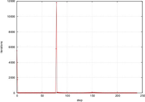
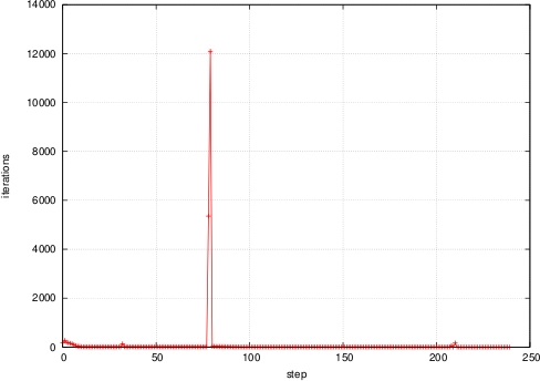
Fig. 6.6: Number of iterations. Left: the initial dual variable is not in the subdifferential of the initial data, which requires more than 50005000 initial iterations for convergence. Right: the initial dual variable is in the subdifferential, which entails fewer initial iterations for convergence (see §6.4).

The result of Theorem 5.1 guarantees convergence of the inner iteration at every step. However, there is no assessment of the speed of convergence. We numerically investigate the effect of the choice of initial condition for the inner loop. Set Ω=(−2,2)\Omega=(-2,2) and u0=χ[−1,1]\textup{{u}}_{0}=\chi_{[-1,1]}. We choose

𝐳01=0,𝐳02={x+2,x∈(−2,−1),−x,x∈(−1,1),x−2,x∈(1,2).{\bf z}_{0}^{1}=0,\quad{\bf z}_{0}^{2}=\begin{cases}x+2,&x\in(-2,-1),\\ -x,&x\in(-1,1),\\ x-2,&x\in(1,2).\end{cases}

It is possible to show that only 𝐳02∈∂Ψ⁡(u0){\bf z}_{0}^{2}\in\partial\Psi(\textup{{u}}_{0}). For h=2−6h=2^{-6}, Δ​t=τ=h/10{\Delta t}=\tau=h/10 and σ=1\sigma=1, Figure 6.6 plots the number of iterations as a function of the step for 𝐳01{\bf z}_{0}^{1} and 𝐳02{\bf z}_{0}^{2}. The number of initial iteration is much higher (more than 50005000) for 𝐳01{\bf z}_{0}^{1} than for 𝐳02{\bf z}_{0}^{2}. Moreover, notice the spike on both graphs at 79 steps. This is due to the fact that, at this step, extinction occurs. From this we conclude that the number of iterations heavily depends on the initial choice of 𝐳0{\bf z}_{0} or, more generally, on 𝝀h0{\boldsymbol{\lambda}}_{h}^{0}. Strategies for choosing it need further investigation.

6.5 Comparison with Regularized Flow

To conclude our discussion, it is imperative to make a comparison between our method and those that involve regularization and show that the advantages in our approach are numerous. Before embarking in such an endeavor, let us recall some properties of regularized flows. The analysis developed in [22] does not provide a clear understanding of the relation between the regularization ϵ\epsilon and the space discretization hh. By means of numerical experiments the authors conclude that ϵ=𝒪⁡(h2)\epsilon={\mathcal{O}}(h^{2}) is the optimal scaling law, see [22, Figures 4–5].

Let us, with the help of the theory developed in §4.2, try to bring some light into this matter. If we denote by uϵ\textup{{u}}_{\epsilon} the solution to (1.1) with regularization Ψϵ​(w)=∫Ωϵ2+|∇w|2\Psi_{\epsilon}(w)=\int_{\Omega}\sqrt{\epsilon^{2}+|\nabla w|^{2}} given by (1.2), [22, Theorem 2] shows that

‖u−uϵ‖L∞​(L2)≤c​ϵ1/2.\|\textup{{u}}-\textup{{u}}_{\epsilon}\|_{L^{\infty}(L^{2})}\leq c\epsilon^{1/2}. (6.1)

If uϵ,hΔ​t⊂𝕍hu_{\epsilon,h}^{\Delta t}\subset{\mathbb{V}}_{h} is the solution to a fully discrete approximation of the regularized flow with Ψϵ,h=Ψϵ\Psi_{\epsilon,h}=\Psi_{\epsilon}, under the assumption that uϵ∈L∞​(0,T,H2​(Ω))\textup{{u}}_{\epsilon}\in L^{\infty}(0,T;{{H}^{2}(\Omega)}) we have

∥uϵ−u^ϵ,hΔ​t∥L∞​(L2)≤c(Δt1/2+h1/2ϵ−α/2).\|\textup{{u}}_{\epsilon}-\widehat{u}_{\epsilon,h}^{\Delta t}\|_{L^{\infty}(L^{2})}\leq c\left({\Delta t}^{1/2}+h^{1/2}\epsilon^{-\alpha/2}\right). (6.2)

To see this it suffices to realize that (4.7) is trivially satisfied and, setting 𝒞h=Πh{\mathcal{C}}_{h}=\Pi_{h} we conclude that (4.8) amounts to

‖ℐh​w−w‖L2≤c​h2​‖w‖H2⟹ε1​(h)=c​h2​‖w‖H2,\|{\mathcal{I}}_{h}w-w\|_{L^{2}}\leq ch^{2}\|w\|_{H^{2}}\quad\Longrightarrow\quad{\varepsilon}_{1}(h)=ch^{2}\|w\|_{H^{2}},

and, since

∫Ω|ϵ2+|∇w1|2−ϵ2+|∇w2|2|≤∫Ω|∇(w1−w2)|,\int_{\Omega}\left|\sqrt{\epsilon^{2}+|\nabla w_{1}|^{2}}-\sqrt{\epsilon^{2}+|\nabla w_{2}|^{2}}\right|\leq\int_{\Omega}\left|\nabla(w_{1}-w_{2})\right|,

we have, for (4.9),

ε2​(h)≤c​h​‖w‖W12.{\varepsilon}_{2}(h)\leq ch\|w\|_{W^{2}_{1}}.

Finally, [21, Theorem 1.2] shows that ‖uϵ‖L2​(H2)≤ϵ−α\|\textup{{u}}_{\epsilon}\|_{L^{2}(H^{2})}\leq\epsilon^{-\alpha} for some α∈ℕ0\alpha\in{\mathbb{N}}_{0}. Combining (6.1) and (6.2) with Theorem 4.5 we conclude

∥u−u^ϵ,hΔ​t∥L∞​(L2)≤c(Δt1/2+ϵ1/2+hϵ−α/2+h1/2),\|\textup{{u}}-\widehat{u}_{\epsilon,h}^{\Delta t}\|_{L^{\infty}(L^{2})}\leq c\left({\Delta t}^{1/2}+\epsilon^{1/2}+h\epsilon^{-\alpha/2}+h^{1/2}\right), (6.3)

which yields the optimal scaling ϵ=𝒪⁡(h21+α)\epsilon={\mathcal{O}}(h^{\frac{2}{1+\alpha}}).

The last ingredient we need to make the comparison is to recall that (cf. [28, Remark 5.3]) in the one dimensional case, i.e., d=1d=1, if the initial data is monotone, it is itself a minimizer of the total variation energy, and so the flow fixes it. In other words, if u0\textup{{u}}_{0} is monotone, then u​(t)=u0\textup{{u}}(t)=\textup{{u}}_{0} for all t>0t>0.

Fig. 6.7: Solution, at T=5T=5, of the TV flow with monotone initial data. Our method (red with ++), regularized flow with ϵ=h\epsilon=h (blue with ×\times) and with ϵ=h2\epsilon=h^{2} (magenta with ∗*). h=2−5h=2^{-5}, Δ​t=2−10{\Delta t}=2^{-10}. The unregularized solution coincides with the exact solution, whereas the regularized flow misses it, although it belongs to the discrete space.

Consider, in Ω=(0,1)\Omega=(0,1), the initial data

u0​(x)={0,x≤12,x−12,12<x≤1.\textup{{u}}_{0}(x)=\begin{cases}0,&x\leq\tfrac{1}{2},\\ x-\tfrac{1}{2},&\tfrac{1}{2}<x\leq 1.\end{cases}

According to the discussion presented above, the solution to (3.2) is u​(t)=u0\textup{{u}}(t)=\textup{{u}}_{0}. Figure 6.7 shows the solution, at T=5T=5, obtained with our method and the regularized flow with ϵ=𝒪⁡(h2)\epsilon={\mathcal{O}}(h^{2}) and ϵ=𝒪⁡(h)\epsilon={\mathcal{O}}(h). The first choice is the one advocated in [22]; while the second is the optimal according to (6.3) provided α=1\alpha=1, which is consistent with Proposition 2.1. In such a case, (6.3) gives the following error estimate

‖u−u^ϵ,hΔ​t‖L∞​(L2)≤c​h1/2,\|\textup{{u}}-\widehat{u}_{\epsilon,h}^{\Delta t}\|_{L^{\infty}(L^{2})}\leq ch^{1/2},

provided ϵ≈h≈Δ​t\epsilon\approx h\approx{\Delta t}. The mesh size is h=2−5h=2^{-5} and the time-step Δ​t=2−10{\Delta t}=2^{-10}. Notice that the requirement Δ​t=𝒪⁡(h2){\Delta t}={\mathcal{O}}(h^{2}), which is needed for L2L^{2}-convergence in the regularized flow (cf. [22, Theorem 4] and [21, Theorem 1.7]), is satisfied.

The advantages of our method are now evident. We do not impose any restriction on the time-step, as opposed to the Δ​t=𝒪⁡(h2){\Delta t}={\mathcal{O}}(h^{2}) that is necessary in regularized methods to guarantee convergence in L2​(Ω){{L}^{2}(\Omega)}. Even if one is willing to settle for convergence in Lp​(Ω)L^{p}(\Omega), with p<d/(d−1)p<d/(d-1), the methods with regularization require that the solution of the regularized flow is in L∞​(0,T,W11​(Ω))∩L∞​(0,T,Hloc1​(Ω))L^{\infty}(0,T;W^{1}_{1}(\Omega))\cap L^{\infty}(0,T;H^{1}_{\text{loc}}(\Omega)). If an error estimate is desired, one must impose that u0∈𝒞2​(Ω¯)\textup{{u}}_{0}\in{\mathcal{C}}^{2}(\bar{\Omega}), and even in that case it is not clear what is the relation between hh, Δ​t{\Delta t} and ϵ\epsilon. In addition to these approximation issues, the regularized flow requires the solution, at each time step, of a nonlinear system and no convergence analysis is provided. In contrast, we have developed and analyzed an inexact iterative scheme for the solution of our problems at each time step, and we have showed its global convergence. To finalize, the result presented in Figure 6.7 shows that the regularized flow misses certain fundamental features of the problem, even in simple cases.

7 Total Variation Minimization

We conclude with yet another application of our result on approximation of functions of bounded variation (Proposition 2.1): we improve on the existing results about total variation minimization. Let g∈L∞​(Ω)g\in L^{\infty}(\Omega) and α>0\alpha>0. Consider Ξ⁡(w)=Ψ⁡(w)+α2​‖w−g‖L22\Xi(w)=\Psi(w)+\tfrac{\alpha}{2}\|w-g\|_{L^{2}}^{2}. Thanks to the fact that this functional is strictly convex there exists a unique ξ∈B​V​(Ω)∩L2​(Ω)\xi\in BV(\Omega)\cap{{L}^{2}(\Omega)} such that

Ξ⁡(ξ)=inf{Ξ⁡(w):w∈L2​(Ω)}<∞.\Xi(\xi)=\inf\left\{\Xi(w):w\in{{L}^{2}(\Omega)}\right\}<\infty. (7.1)

Here we are interested in the approximation of ξ\xi by elements of 𝕍h{\mathbb{V}}_{h}. Since 𝕍h{\mathbb{V}}_{h} is finite dimensional, there is a unique ξh∈𝕍h\xi_{h}\in{\mathbb{V}}_{h} such that

Ξ⁡(ξh)=inf{Ξ⁡(wh):w∈𝕍h}<∞.\Xi(\xi_{h})=\inf\left\{\Xi(w_{h}):w\in{\mathbb{V}}_{h}\right\}<\infty. (7.2)

The main approximation properties of ξh\xi_{h} are detailed in the following.

Theorem 7.1 (Convergence of discrete minimizers).

Assume that Ω\Omega is star shaped with respect to a point. Let ξ∈B​V​(Ω)∩L∞​(Ω)\xi\in BV(\Omega)\cap L^{\infty}(\Omega) and ξh∈𝕍h\xi_{h}\in{\mathbb{V}}_{h} be defined as in (7.1) and (7.2), respectively. Then

‖ξ−ξh‖L2≤c​h1/4.\|\xi-\xi_{h}\|_{L^{2}}\leq ch^{1/4}.
Proof.

We adapt the ideas presented in [7, Theorem 3.1]. Let ϵ>0\epsilon>0 and ξϵ∈𝒞∞​(Ω)\xi_{\epsilon}\in{\mathcal{C}}^{\infty}(\Omega) be an approximation of ξ\xi that satisfies all the properties stated in Proposition 2.1. Owing to the strict convexity of Ξ\Xi and the fact that ξh\xi_{h} is a discrete minimizer, we have

α2​‖ξ−ξh‖L22\displaystyle\frac{\alpha}{2}\|\xi-\xi_{h}\|_{L^{2}}^{2} ≤Ξ⁡(ξh)−Ξ⁡(ξ)≤Ξ⁡(Πh​ξϵ)−Ξ⁡(ξ)\displaystyle\leq\Xi(\xi_{h})-\Xi(\xi)\leq\Xi(\Pi_{h}\xi_{\epsilon})-\Xi(\xi)
=(∥∇Πhξϵ∥L1−|Dξ|(Ω))+α2(∥Πhξϵ−g∥L22−∥ξ−g∥L22)=𝒜1+𝒜2,\displaystyle=\left(\|\nabla\Pi_{h}\xi_{\epsilon}\|_{L^{1}}-|{\textup{D}}\xi|(\Omega)\right)+\frac{\alpha}{2}\left(\|\Pi_{h}\xi_{\epsilon}-g\|_{L^{2}}^{2}-\|\xi-g\|_{L^{2}}^{2}\right)={\mathcal{A}}_{1}+{\mathcal{A}}_{2},

where Πh\Pi_{h} is the Clément interpolation operator [15]. Let us look at each one of the terms in this last inequality:

  1. 𝒜1{\mathcal{A}}_{1}:

    We add and subtract the W11W^{1}_{1}-seminorm of ξϵ\xi_{\epsilon} and use its approximation properties with respect to total variation along with the approximation properties of Πh\Pi_{h} described in (2.8):

    𝒜1≤‖∇(Πh​ξϵ−ξϵ)‖L1+‖∇ξϵ‖L1−|D​ξ|(Ω)≤c⁡(hϵ+ϵ)​|D​ξ|​(Ω).{\mathcal{A}}_{1}\leq\|\nabla(\Pi_{h}\xi_{\epsilon}-\xi_{\epsilon})\|_{L^{1}}+\|\nabla\xi_{\epsilon}\|_{L^{1}}-|{\textup{D}}\xi|(\Omega)\leq c\left(\frac{h}{\epsilon}+\epsilon\right)|{\textup{D}}\xi|(\Omega).
  2. 𝒜2{\mathcal{A}}_{2}:

    We, again, use the approximation properties of ξϵ\xi_{\epsilon} and the fact that ξ\xi and gg are essentially bounded, say by a constant c>0c>0,

    𝒜2≤c​α2​(‖ℐh​ξϵ−ξϵ‖L1+‖ξϵ−ξ‖L1)≤c⁡(h2ϵ+ϵ)​|D​ξ|​(Ω).{\mathcal{A}}_{2}\leq\frac{c\alpha}{2}\left(\|{\mathcal{I}}_{h}\xi_{\epsilon}-\xi_{\epsilon}\|_{L^{1}}+\|\xi_{\epsilon}-\xi\|_{L^{1}}\right)\leq c\left(\frac{h^{2}}{\epsilon}+\epsilon\right)|{\textup{D}}\xi|(\Omega).

Setting ϵ=h12\epsilon=h^{\frac{1}{2}} we obtain the result. ∎

Remark 7.2 (Convergence of total variation minimization).

Theorem 7.1 is, in a sense, an improvement over the original result of [7], at least for star shaped domains, and under the boundedness assumptions on gg and ξ\xi. If ξ∈B∞s​(L2​(Ω))\xi\in B^{s}_{\infty}({{L}^{2}(\Omega)}) for some s∈(0,1]s\in(0,1], and relying on the results of [37], [7, Theorem 3.1] proves the estimate

‖ξ−ξh‖L2≤c​hs2​(1+s),\|\xi-\xi_{h}\|_{L^{2}}\leq ch^{\frac{s}{2(1+s)}},

so that the best possible rate of convergence is 𝒪⁡(h1/4){\mathcal{O}}(h^{1/4}), which is what we obtain, but with lower regularity. To understand this regularity assumption it suffices to recall that B​V​(Ω)∩L∞​(Ω)↪B∞s​(L2​(Ω))BV(\Omega)\cap L^{\infty}(\Omega)\hookrightarrow B^{s}_{\infty}(L^{2}(\Omega)) for s≤12s\leq\tfrac{1}{2} (see [36, Lemma 38.1] for a proof and, in some sense, the converse inclusion). The key step that allowed us to reduce the smoothness assumption is Proposition 2.1. In addition, the proof of Theorem 7.1 shows that if we had a TV-diminishing interpolant, we would obtain

‖ξ−ξh‖L2≤c​h1/2,\|\xi-\xi_{h}\|_{L^{2}}\leq ch^{1/2},

which is an optimal error estimate for ξ∈B∞s​(L2​(Ω))\xi\in B^{s}_{\infty}({{L}^{2}(\Omega)}). Such a construction is presented in [32].

References

  • [1] L. Ambrosio, N. Fusco, and D. Pallara, Functions of bounded variation and free discontinuity problems, Oxford Mathematical Monographs, The Clarendon Press Oxford University Press, New York, 2000.
  • [2] F. Andreu-Vaillo, V. Caselles, and J.M. Mazón, Parabolic quasilinear equations minimizing linear growth functionals, vol. 223 of Progress in Mathematics, Birkhäuser Verlag, Basel, 2004.
  • [3] G. Anzellotti, Pairings between measures and bounded functions and compensated compactness, Ann. Mat. Pura Appl. (4), 135 (1983), pp. 293–318 (1984).
  • [4] W. Bangerth, R. Hartmann, and G. Kanschat, deal.II Differential Equations Analysis Library, Technical Reference. http://www.dealii.org.
  • [5]  , deal.II — a general-purpose object-oriented finite element library, ACM Trans. Math. Softw., 33 (2007).
  • [6] V. Barbu, Nonlinear differential equations of monotone types in Banach spaces, Springer Monographs in Mathematics, Springer, New York, 2010.
  • [7] S. Bartels, Total variation minimization with finite elements: Convergence and iterative solution, SIAM Journal on Numerical Analysis, 50 (2012), pp. 1162–1180.
  • [8] G. Bellettini, V. Caselles, and M. Novaga, The total variation flow in ℝN\mathbb{R}^{N}, J. Differential Equations, 184 (2002), pp. 475–525.
  • [9] M. Breuß, T. Brox, A. Bürgel, T. Sonar, and J. Weickert, Numerical aspects of TV flow, Numer. Algorithms, 41 (2006), pp. 79–101.
  • [10] H. Brézis, Opérateurs maximaux monotones et semi-groupes de contractions dans les espaces de Hilbert, North-Holland Publishing Co., Amsterdam, 1973. North-Holland Mathematics Studies, No. 5. Notas de Matemática (50).
  • [11] M. Burger, K. Frick, S. Osher, and O. Scherzer, Inverse total variation flow, Multiscale Model. Simul., 6 (2007), pp. 365–395 (electronic).
  • [12] A. Chambolle and T. Pock, A first-order primal-dual algorithm for convex problems with applications to imaging, J. Math. Imaging Vision, 40 (2011), pp. 120–145.
  • [13] R.H. Chan, Y. Dong, and M. Hintermüller, An efficient two-phase L1{\rm L}^{1}-TV method for restoring blurred images with impulse noise, IEEE Trans. Image Process., 19 (2010), pp. 1731–1739.
  • [14] P.G. Ciarlet, The Finite Element Method for Elliptic Problems, North Holland, Amsterdam, 1978.
  • [15] Ph. Clément, Approximation by finite element functions using local regularization, Rev. Française Automat. Informat. Recherche Opérationnelle Sér. RAIRO Analyse Numérique, 9 (1975), pp. 77–84.
  • [16] D.C. Dobson and C.R. Vogel, Convergence of an iterative method for total variation denoising, SIAM J. Numer. Anal., 34 (1997), pp. 1779–1791.
  • [17] V. Duval, J.-F. Aujol, and Y. Gousseau, The TVL1 model: a geometric point of view, Multiscale Model. Simul., 8 (2009), pp. 154–189.
  • [18] I. Ekeland and R. Témam, Convex analysis and variational problems, vol. 28 of Classics in Applied Mathematics, Society for Industrial and Applied Mathematics (SIAM), Philadelphia, PA, english ed., 1999. Translated from the French.
  • [19] C.M. Elliott and S.A. Smitheman, Numerical analysis of the TV regularization and H−1H^{-1} fidelity model for decomposing an image into cartoon plus texture, IMA J. Numer. Anal., 29 (2009), pp. 651–689.
  • [20] A. Ern and J.-L. Guermond, Theory and practice of finite elements, vol. 159 of Applied Mathematical Sciences, Springer-Verlag, New York, 2004.
  • [21] X. Feng and A. Prohl, Analysis of total variation flow and its finite element approximations, M2AN Math. Model. Numer. Anal., 37 (2003), pp. 533–556.
  • [22] X. Feng, M. von Oehsen, and A. Prohl, Rate of convergence of regularization procedures and finite element approximations for the total variation flow, Numer. Math., 100 (2005), pp. 441–456.
  • [23] P.-W. Fok, R.R. Rosales, and D. Margetis, Facet evolution on supported nanostructures: Effect of finite height, Phys. Rev. B, 78 (2008), p. 235401.
  • [24] G.B. Folland, Real analysis, Pure and Applied Mathematics (New York), John Wiley & Sons Inc., New York, second ed., 1999. Modern techniques and their applications, A Wiley-Interscience Publication.
  • [25] E.S. Fu, D.-J. Liu, M.D. Johnson, J.D. Weeks, and E.D. Williams, The effective charge in surface electromigration, Surface Science, 385 (1997), pp. 259 – 269.
  • [26] M.-H. Giga and Y. Giga, Very singular diffusion equations: second and fourth order problems, Jpn. J. Ind. Appl. Math., 27 (2010), pp. 323–345.
  • [27] M.-H. Giga, Y. Giga, and R. Kobayashi, Very singular diffusion equations, in Taniguchi Conference on Mathematics Nara ’98, vol. 31 of Adv. Stud. Pure Math., Math. Soc. Japan, Tokyo, 2001, pp. 93–125.
  • [28] R. Hardt and X. Zhou, An evolution problem for linear growth functionals, Comm. Partial Differential Equations, 19 (1994), pp. 1879–1907.
  • [29] R. Kobayashi, J.A. Warren, and W.C. Carter, A continuum model of grain boundaries, Physica D: Nonlinear Phenomena, 140 (2000), pp. 141 – 150.
  • [30] R.V. Kohn and H.M. Versieux, Numerical analysis of a steepest-descent PDE model for surface relaxation below the roughening temperature, SIAM J. Numer. Anal., 48 (2010), pp. 1781–1800.
  • [31] W.G. Litvinov, T. Rahman, and X.-C. Tai, A modified TV-Stokes model for image processing, SIAM J. Sci. Comput., 33 (2011), pp. 1574–1597.
  • [32] R.H. Nochetto and A.J. Salgado, A TV diminishing interpolation operator and applications. Submitted, arXiv:1211.1069, 2012.
  • [33] R.H. Nochetto, G. Savaré, and C. Verdi, A posteriori error estimates for variable time-step discretizations of nonlinear evolution equations, Comm. Pure Appl. Math., 53 (2000), pp. 525–589.
  • [34] L.I. Rudin, S. Osher, and E. Fatemi, Nonlinear total variation based noise removal algorithms, Physica D: Nonlinear Phenomena, 60 (1992), pp. 259–268.
  • [35] J. Rulla, Error analysis for implicit approximations to solutions to Cauchy problems, SIAM J. Numer. Anal., 33 (1996), pp. 68–87.
  • [36] L. Tartar, An introduction to Sobolev spaces and interpolation spaces, vol. 3 of Lecture Notes of the Unione Matematica Italiana, Springer, Berlin, 2007.
  • [37] J. Wang and B.J. Lucier, Error bounds for finite-difference methods for Rudin-Osher-Fatemi image smoothing, SIAM J. Numer. Anal., 49 (2011), pp. 845–868.
  • [38] W.P. Ziemer, Weakly differentiable functions, vol. 120 of Graduate Texts in Mathematics, Springer-Verlag, New York, 1989. Sobolev spaces and functions of bounded variation.