Characterising Steady-State Topologies of
SIS Dynamics on Adaptive Networks

Gross et al. ([1]) incorporated disease awareness into conventional SIS dynamics by allowing susceptibles to evade infection through retracting links from infected neighbours and rewiring them to randomly selected susceptibles. Using the moment closure from [3] to obtain a pair approximation model (PA) of the process, the time evolution of the fraction of infected $i$ is coupled to that of the densities $l_{\mathrm{XY}}$ of links connecting nodes of type $X$ and $Y$ ($\{X,Y\}\in\{S\mathrm{=susceptible},I\mathrm{=infected}\}$). Apart from the conserved link density $l=l_{\mathrm{SS}}+l_{\mathrm{SI}}+l_{\mathrm{II}}$, the model can be parameterised by $\rho,\omega\in[0,1]$, with rewiring, infection and recovery rates given by $\omega,\left(1-\omega\right)\rho$ and $\left(1-\omega\right)\left(1-\rho\right)$, respectively.

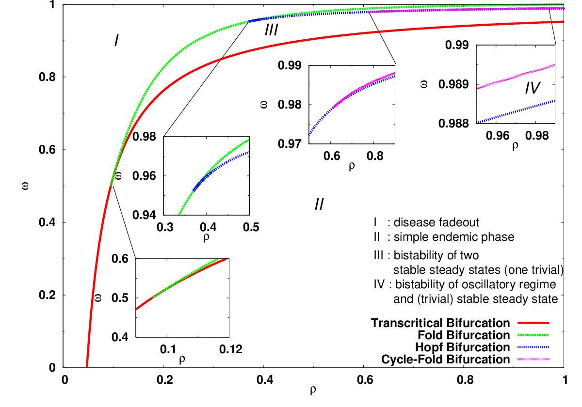
The full phase diagram is presented in Fig. 1; for any $l\geq 0.5$ the minimum rewiring rate for bistability to arise is $\omega\!=\!0.5$. The transcritical bifurcation, serving as the epidemic threshold and approximated in [1], occurs at exactly $\omega=1-1/\left(\rho\left[2l+1\right]\right)$.

We have checked the steady state values for densities and pairs predicted by the PA against simulations on networks with $N=10^{4}$ nodes, taking as initial conditions the predicted steady-state value of $i$, with infected and susceptibles initially randomly distributed on a Poisson network of average degree $\langle k\rangle=2l=20$. In the simple endemic phase, prevalence and link densities of numerical simulations and model predictions agree reasonably well. At $\omega=\rho/\left(1+\rho\right)$, i.e. when the infection rate is equal to the rewiring rate, the pair approximation model correctly predicts $i$ and the mean degrees of both susceptibles and infected.

The steady-state degree distributions (DD) of the subnetworks of infected and susceptibles - as well as that of the complete network - are shown in Figs. 2 and 3. Independently from topological starting conditions in the simple endemic phase, the final topology (as described by several standard measures) settles down to a characteristic state (Fig. 2).

Let $\langle k_{\mathrm{S}}\rangle=\sum_{k}ks_{k}/s$ and $\langle k_{\mathrm{I}}\rangle=\sum_{k}ki_{k}/i$ be the average degree of susceptible and infected, where $a_{k}$ is the fraction of the total number of nodes which are in state $a$ and have degree $k$, $a\in\{s,\kern 5.0pti\}$. Hence the average degree of the network is $\langle k\rangle=s\langle k_{\mathrm{S}}\rangle+i\langle k_{\mathrm{I}}\rangle$. We have also, by definition, $s\langle k_{\mathrm{S}}\rangle=2l_{\mathrm{SS}}+l_{\mathrm{SI}}$ and $i\langle k_{\mathrm{I}}\rangle=2l_{\mathrm{II}}+l_{\mathrm{SI}}$, so that the average degrees of the two subnetworks in the steady state are determined by the equilibrium values of the PA in the region where the moment closure from [3] holds.

Rewiring induces infection-status clustering ([1]); in the PA, the difference of the mean degrees of susceptible and infected nodes is independent of the link density and given by

Thus only for $\omega>\rho/\left(1+\rho\right)$ does rewiring yield a bigger mean degree in susceptibles than in infected (Fig. 3). Again $\omega$ and $\rho$ given by $\omega=\rho/\left(1+\rho\right)$ enjoy a special status, in that then the mean degrees of the $S$- and $I$-ensemble are the same, as are their degree distributions and every other topology-related statistics we measured.

Depending on a node’s status, it will either gain in degree (when susceptible) or lose links (when infected). Characterising such a typical node cycle gives important single-node characteristics describing its degree during and lifetime of each stage, as well as a means to determine the overall infection-class degree distributions.

The time evolution of the number of susceptible and infected neighbours $l_{\mathrm{S}}(t)$ and $l_{\mathrm{I}}(t)$ of a typical node is

in its susceptible stage (phase I) and

when it is infected (phase II). The constants $\lambda_{i}\in\mathbb{R}_{\geq 0}$ and $c_{j}\in\mathbb{R}$ are comprised of $\omega,\rho$, the steady-state values of $l_{\mathrm{SI}}$ and $s$ (computable through the PA), as well as the four initial conditions to be determined by a cyclic closure of (1) and (2).

A crucial ingredient is the mean-field approximation for the average lifetime $\tau_{\mathrm{S}}$ of a susceptible; $\tau_{\mathrm{S}}=s/\left(\left[1-\omega\right]\rho l_{\mathrm{SI}}\right)$ turns out to be a very good one throughout parameter space. This is due to the fact that over a susceptible’s lifetime, there is no noticable degree-, time- or any other correlation in the $S$-nodes rewired to it, particularly not in the number of their $I$-neighbours. Hence the node-cycle model also accurately describes regimes with very high $\omega$. There, the near-linear degree growth and the trough of $l_{\mathrm{I}}(t)$ around $\tau_{\mathrm{S}}$ in the first phase are well-captured by our equations. So is the rapid rewiring away of $l_{\mathrm{S}}$-links in the initial stage of the second phase, followed by slow degree loss through recovery and subsequent rewiring (Fig. 4a and 4b).

Let $l_{\mathrm{SI}_{k}}$ be the fraction of the $SI$-link density with $I$-nodes of degree $k$. Denote also by $l_{\mathrm{S}_{k}\mathrm{I}}$ the number of $SI$-links whose $S$-node is of degree $k$, divided by the number of nodes $N$. In order to describe the infection-class subnetworks, we must, instead of considering the pairwise equations in [1], deal with the dynamics of each degree class of infected and susceptibles. For the processes and rates we are considering, this is given by

Financial support from the Foundation of the University of Lisbon and the Portuguese Foundation for Science and Technology (FCT) under contract POCTI/ISFL/2/618 is gratefully acknowledged. The first and second authors (SW and TA) were also supported by FCT under grants SFRH/BD/45179/2008 and CFTC-618-BII-02/08.

References

- [1] Thilo Gross, Carlos Dommar D’Lima, and Bernd Blasius. Epidemic dynamics on an adaptive network. Physical Review Letters, 96:208701, 2006.
- [2] Leah B. Shaw and Ira B. Schwartz. Fluctuating epidemics on adaptive networks. Phys. Rev. E, 77:066101, 2008.
- [3] M. J. Keeling and K. T. D. Eames. Networks and epidemic models. Journal of the Royal Society Interface, 2:295–307, 2005.
- [4] Eusebius Doedel et al. AUTO-07p Bifurcation Software. Concordia University, Montreal, 2007.