Universality for random matrices and log-gases
Lecture Notes for Current Developments in
Mathematics, 2012
Abstract
Eugene Wigner’s revolutionary vision predicted that the energy levels of large complex quantum systems exhibit a universal behavior: the statistics of energy gaps depend only on the basic symmetry type of the model. These universal statistics show strong correlations in the form of level repulsion and they seem to represent a new paradigm of point processes that are characteristically different from the Poisson statistics of independent points.
Simplified models of Wigner’s thesis have recently become mathematically accessible. For mean field models represented by large random matrices with independent entries, the celebrated Wigner-Dyson-Gaudin-Mehta (WDGM) conjecture asserts that the local eigenvalue statistics are universal. For invariant matrix models, the eigenvalue distributions are given by a log-gas with potential and inverse temperature . corresponding to the orthogonal, unitary and symplectic ensembles. For , there is no natural random matrix ensemble behind this model, but the analogue of the WDGM conjecture asserts that the local statistics are independent of .
In these lecture notes we review the recent solution to these conjectures for both invariant and non-invariant ensembles. We will discuss two different notions of universality in the sense of (i) local correlation functions and (ii) gap distributions. We will demonstrate that the local ergodicity of the Dyson Brownian motion is the intrinsic mechanism behind the universality. In particular, we review the solution of Dyson’s conjecture on the local relaxation time of the Dyson Brownian motion. Additionally, the gap distribution requires a De Giorgi-Nash-Moser type Hölder regularity analysis for a discrete parabolic equation with random coefficients. Related questions such as the local version of Wigner’s semicircle law and delocalization of eigenvectors will also be discussed. We will also explain how these results can be extended beyond the mean field models, especially to random band matrices.
AMS Subject Classification (2010): 15B52, 82B44
Keywords: -ensemble, local semicircle law, Dyson Brownian motion. De Giorgi-Nash-Moser theory.
1 Introduction
1.1 The pioneering vision of Wigner
“Perhaps I am now too courageous when I try to guess the distribution of the distances between successive levels (of energies of heavy nuclei). Theoretically, the situation is quite simple if one attacks the problem in a simpleminded fashion. The question is simply what are the distances of the characteristic values of a symmetric matrix with random coefficients.”
Eugene Wigner on the Wigner surmise, 1956
Large complex systems often exhibit remarkably simple universal patterns as the number of degrees of freedom increases. The simplest example is the central limit theorem: the fluctuation of the sums of independent random scalars, irrespective of their distributions, follows the Gaussian distribution. The other cornerstone of probability theory identifies the Poisson point process as the universal limit of many independent point-like events in space or time. These mathematical descriptions assume that the original system has independent (or at least weakly dependent) constituents. What if independence is not a realistic approximation and strong correlations need to be modelled? Is there a universality for strongly correlated models?
At first sight this seems an impossible task. While independence is a unique concept, correlations come in many different forms; a-priori there is no reason to believe that they all behave similarly. Nevertheless they do, according to the pioneering vision of Wigner [86] at least if they originate from certain physical systems and if the “right” question is asked. The actual correlated system he studied was the energy levels of heavy nuclei. Looking at spectral measurement data, it is obvious that the eigenvalue density (or density of states, as it is called in physics) heavily depends on the system. But Wigner asked a different question: what about the distribution of the rescaled energy gaps? He discovered that the difference of consecutive energy levels, after rescaling with the local density, shows a surprisingly universal behavior. He even predicted a universal law, given by the simple formula (called the Wigner surmise),
| (1.1) |
where denote the rescaling of the actual energy levels by the density of states near the energy . This law is characteristically different from the gap distribution of the Poisson process which is the exponential distribution, . The prefactor in (1.1) indicates a level repulsion for the point process , i.e. the eigenvalues are strongly correlated.
Comparing measurement data from various experiments, Wigner’s pioneering vision was that the energy gap distribution (1.1) of complicated quantum systems is essentially universal; it depends only on the basic symmetries of model (such as time-reversal invariance). This thesis has never been rigorously proved for any realistic physical system but experimental data and extensive numerics leave no doubt on its correctness (see [64] for an overview).
Wigner not only predicted universality in complicated systems, but he also discovered a remarkably simple mathematical model for this new phenomenon: the eigenvalues of large random matrices. For practical purposes, Hamilton operators of quantum models are often approximated by large matrices that are obtained from some type of discretization of the original continuous model. These matrices have specific forms dictated by physical rules. Wigner’s bold step was to neglect all details and consider the simplest random matrix whose entries are independent and identically distributed. The only physical property he retained was the basic symmetry class of the system; time reversal physical models were modelled by real symmetric matrices, while systems without time reversal symmetry (e.g. with magnetic fields) were modelled by complex Hermitian matrices. As far as the gap statistics are concerned, this simple-minded model reproduced the behavior of the complex quantum systems! The universal behavior extends to the joint statistics of several consecutive gaps which are essentially equivalent to the local correlation functions of the point process . From mathematical point of view, a universal strongly correlated point process was found. The natural representatives of these universality classes are the random matrices with independent identically distributed Gaussian entries. These are called the Gaussian orthogonal ensemble (GOE) and the Gaussian unitary ensemble (GUE) in case of real symmetric and complex Hermitian matrices, respectively.
Since Wigner’s discovery random matrix statistics are found everywhere in physics and beyond, wherever nontrivial correlations prevail. Among many other applications, random matrix theory (RMT) is present in chaotic quantum systems in physics, in principal component analysis in statistics, in communication theory and even in number theory. In particular, the zeros of the Riemann zeta function on the critical line are expected to follow RMT statistics due to a spectacular result of Montgomery [68].
In retrospect, Wigner’s idea should have received even more attention. For centuries, the primary territory of probability theory was to model uncorrelated or weakly correlated systems. The surprising ubiquity of random matrix statistics is a strong evidence that it plays a similar fundamental role for correlated systems as Gaussian distribution and Poisson point process play for uncorrelated systems. RMT seems to provide essentially the only universal and generally computable pattern for complicated correlated systems.
In fact, a few years after Wigner’s seminal paper [86], Gaudin [52] has discovered another remarkable property of this new point process: the correlation functions have a determinantal structure, at least if the distributions of the matrix elements are Gaussian. The algebraic identities within the determinantal form opened up the route to calculations and to obtain explicit formulas for local correlation functions. In particular, the gap distribution for the complex Hermitian case is given by a Fredholm determinant involving Hermite polynomials. In fact, Hermite polynomials were first introduced in the context of random matrices by Mehta and Gaudin [66] earlier. Dyson and Mehta [65, 23, 25] have later extended this exact calculation to correlation functions and to other symmetry classes. When compared with the exact formula, the Wigner surmise (1.1), based upon a simple matrix model, turned out to be quite accurate. While the determinantal structure is present only in Gaussian Wigner matrices, the paradigm of local universality predicts that the formulas for the local eigenvalue statistics obtained in the Gaussian case hold for general distributions as well.
1.2 Physical models
The ultimate mathematical goal is to prove Wigner’s vision for a very large class of realistic quantum mechanical models. This is extremely hard, since the local statistics involve tracking individual eigenvalues in the bulk spectrum. Wigner’s original model, the energy levels of heavy nuclei, is a strongly interacting many-body quantum system. The rigorous analysis of such model with the required precision is beyond the reach of current mathematics.
A much simpler question is to neglect all interactions and to study the natural one-body quantum model, the Schrödinger operator with a potential on . The complexity comes from assuming that is generic in some sense, in particular to exclude models with additional symmetries that may lead to non-universal eigenvalue correlations. Two well-studied examples are (i) the random Schrödinger operators where is a random field with a short range correlation, and (ii) quantum chaos models, where is generic but fixed and the statistical ensemble is generated by sampling the spectrum in small spectral windows at high energies (an alternative formulation uses the semiclassical limit).
Unfortunately, there are essentially no rigorous results on local spectral universality even in these one-body models. Random Schrödinger operators are conjectured to exhibit a metal-insulator transition that was discovered by Anderson [4]. The high disorder regime is relatively well understood since the seminal work of Fröhlich and Spencer [50] (an alternative proof is given by Aizenman and Molchanov [1]). However, in this regime the eigenfunctions are localized and thus eigenfunctions belonging to neighboring eigenvalues are typically spatially separated, hence uncorrelated. Therefore, due to localization, the system does not have sufficient correlation to fall into the RMT universality class; in fact the local eigenvalue statistics follow the Poisson process [67]. In contrast, in the low disorder regime, starting from three spatial dimension and away from the spectral edges, the eigenfunctions are conjectured to be delocalized (extended states conjecture). Spatially overlapping eigenfunctions introduce correlations among eigenvalues and it is expected that the local statistics are given by RMT. In the theoretical physics literature, the existence of the delocalized regime and its RMT statistics are considered as facts, supported both by non-rigorous arguments and numerics. One of the most intriguing approach is via supersymmetric (SUSY) functional integrals that remarkably reproduce all formulas obtained by the determinantal calculations in much more general setup but in a non-rigorous way due to neglecting highly oscillatory terms. The rigorous mathematics seriously lags behind these developments; even the existence of the delocalized regime is not proven, let alone detailed spectral statistics.
Judged from the horizons of theoretical physics, rigorous mathematics does not fare much better in the quantum chaos models either. The grand vision is that the quantization of an integrable classical Hamiltonian system exhibits Poisson eigenvalue statistics and a chaotic classical system gives rise to RMT statistics [10, 8]. While Poisson statistics have been shown to emerge some specific integrable models [79, 76, 63], there is no rigorous result on the RMT statistics. Recently there has been a remarkable mathematical progress in quantum unique ergodicity (QUE) that predicts that all eigenfunctions of chaotic systems are uniformly distributed all over the space, at least in some macroscopic sense. For arithmetic domains QUE has been proved in [61]. For general manifolds much less is known, but a lower bound on the topological entropy of the support of the limiting densities of eigenfunctions excludes that eigenfunctions are supported only on a periodic orbit [2]. Very roughly, QUE can be considered as the analogue of the extended states for random Schrödinger operators. Theoretically, the overlap of eigenfunctions should again lead to correlations between neighboring eigenvalues, but their direct quantitative analysis would require a much more precise understanding of the eigenfunctions.
1.3 Random matrix ensembles
In these lectures we consider even simpler models to test Wigner’s universality hypothesis, namely the random matrix ensemble itself. The main goal is to show that their eigenvalues follow the local statistics of the Gaussian Wigner matrices which have earlier been computed explicitly by Dyson, Gaudin and Mehta. The statement that the local eigenvalue statistics is independent of the law of the matrix elements is generally referred to as the universality conjecture of random matrices and we will call it the Wigner-Dyson-Gaudin-Mehta conjecture. It was first formulated in Mehta’s treatise on random matrices [64] in 1967 and has remained a key question in the subject ever since. The goal of these lecture notes is to review the recent progress that has led to the proof of this conjecture and we sketch some important ideas. We will, however, not be able to present all aspects of random matrices and we refer the reader to recent comprehensive books [17, 19, 3].
1.3.1 Wigner ensembles
To make the problem simpler, we restrict ourselves to either real symmetric or complex Hermitian matrices so that the eigenvalues are real. The standard model consists of square matrices with matrix elements having mean zero and variance , i.e.,
| (1.2) |
The matrix elements , , are real or complex independent random variables subject to the symmetry constraint . These ensembles of random matrices are called (standard) Wigner matrices. We will always consider the limit as the matrix size goes to infinity, i.e., . Every quantity related to depends on , so we should have used the notation and , etc., but for simplicity we will omit in the notation.
In Section 2 we will also consider generalizations of these ensembles, where we allow the matrix elements to have different distributions (but retaining independence). The main motivation is to depart from the mean-field character of the standard Wigner matrices, where the quantum transition amplitudes between any two sites have the same statistics. The most prominent example is the random band matrix ensemble (see Example 2.1) that naturally interpolates between standard Wigner matrices and random Schrödinger operators with a short range hopping mechanism (see [80] for an overview).
The first rigorous result about the spectrum of a random matrix of this type is the famous Wigner semicircle law [86] which states that the empirical density of the eigenvalues, , under the normalization (1.2), is given by
| (1.3) |
in the weak limit as . The limit density is independent of the details of the distribution of .
The Wigner surmise (1.1) is a much finer problem since it concerns individual eigenvalues and not only their behavior on macroscopic scale. To understand it, we introduce correlation functions. If denotes the joint probability density of the (unordered) eigenvalues, then the -point correlation functions (marginals) are defined by
| (1.4) |
To keep this introduction simple, we state the corresponding results in terms of the eigenvalue correlation functions for Hermitian matrices. In the Gaussian case (GUE) the joint probability density of the eigenvalues can be expressed explicitly as
| (1.5) |
where the normalization constant can be computed explicitly. The Vandermonde determinant structure allows one to compute the -point correlation functions in the large limit via Hermite polynomials that are the orthogonal polynomials with respect to the Gaussian weight function.
The result of Dyson, Gaudin and Mehta asserts that for any fixed energy in the bulk of the spectrum, i.e., , the small scale behavior of is given explicitly by
| (1.6) |
where is the celebrated sine kernel
| (1.7) |
Note that the limit in (1.6) is independent of the energy as long as it lies in the bulk of the spectrum. The rescaling by a factor of the correlation functions in (1.6) corresponds to the typical distance between consecutive eigenvalues and we will refer to the law under such scaling as local statistics. Note that the correlation functions do not factorize, i.e. the eigenvalues are strongly correlated despite that the matrix elements are independent. Similar but more complicated formulas were obtained for symmetric matrices and also for the self-dual quaternion random matrices which is the third symmetry class of random matrix ensembles.
The convergence in (1.6) holds for each fixed and uniformly in in any compact subset of . Fix now compact subsets in . From (1.6) one can compute the distribution of the number of the rescaled eigenvalues in around a fixed energy . The limit of the joint probabilities
| (1.8) |
is given as derivatives of a Fredholm determinant involving the sine kernel. Clearly (1.8) gives a complete local description of the rescaled eigenvalues as a point process around a fixed energy . In particular it describes the distribution of the eigenvalue gap that contains a fixed energy . However, (1.8) does not determine the distribution of the gap with a fixed label, e.g. the gap . Only the cumulative statistics of many consecutive gaps can be deduced, see [17] for a precise formulation. The slight discrepancy between the statements at fixed energy and with fixed label leads to involved technical complications.
1.3.2 Invariant ensembles
The explicit formula (1.5) is special for Gaussian Wigner matrices; if are independent but non-Gaussian, then no analogous explicit formula is known for the joint probability density. Gaussian Wigner matrices have this special property because their distribution is invariant under base transformation. The derivation of (1.5) relies on the fact that in the diagonalization of , where is diagonal and is unitary, the distributions of and decouple. The Gaussian measure of with the normalization (1.2) can also be expressed as
| (1.9) |
where is the Lebesgue measure on hermitian matrices. The Vandermonde determinant in (1.5) originates from the integrating the Jacobian over the unitary group. Similar argument holds for real symmetric matrices with orthogonal conjugations, the only difference is the exponent 2 of the Vandermonde determinant becomes 1. The exponent is 4 for the third symmetry class of Wigner matrices, the self-dual quaternion matrices with symmetry group being the symplectic matrices (Gaussian symplectic ensemble, GSE).
Starting from (1.5), there are two natural generalizations of Gaussian Wigner matrices. One direction is the Wigner matrices with non-Gaussian but independent entries that we have already introduced in Section 1.3.1. Another direction is to consider a more general real function of instead of the quadratic in (1.9). Since invariance still holds, , the same argument gives (1.5), with instead of , for the correlation functions of . These are called invariant ensembles with potential . Their matrix elements are in general correlated except in the Gaussian case.
Invariant ensembles in all three symmetry classes can be given simultaneously by the probability measure
where is the size of the matrix , is a real valued potential and is the normalization constant. The positive parameter is determined by the symmetry class, its value is 1, 2 or 4, for real symmetric, complex hermitian and self-dual quaternion matrices, respectively. The Lebesgue measure is understood over the matrices in the same class. The probability distribution of the eigenvalues is given by the explicit formula (c.f. (1.5))
| (1.10) |
The key structural ingredient of this formula, the logarithmic interaction that gives rise to the the Vandermonde determinant, is the same as in the Gaussian case, (1.5). Thus all previous computations, developed for the Gaussian case, can be carried out for , provided that the Gaussian weight function for the orthogonal polynomials is replaced with the function . The analysis of the correlation functions depends critically on the the asymptotic properties of the corresponding orthogonal polynomials.
While the asymptotics of the Hermite polynomial for the Gaussian case are well-known, the extension of the necessary analysis to a general potential is a demanding task; important progress was made since the late 1990’s by Fokas-Its-Kitaev [49], Bleher-Its [9], Deift et. al. [17, 20, 21], Pastur-Shcherbina [71, 72] and more recently by Lubinsky [62]. These results concern the simpler case. For , the universality was established only quite recently for analytic with additional assumptions [18, 19, 59, 78] using earlier ideas of Widom [85]. The final outcome of these sophisticated analyses is that universality holds for the measure (1.10) in the sense that the short scale behavior of the correlation functions is independent of the potential (with appropriate assumptions) provided that is one of the classical values, i.e., , that corresponds to an underlying matrix ensemble.
Notwithstanding matrix ensembles or orthogonal polynomials, the measure (1.10) on points is perfectly well defined for any . It can be interpreted as the Gibbs measure for a system of particles with external potential and with a logarithmic interaction (log-gas) at inverse temperature . From this point of view is a continuous parameter and the classical values play apparently no distinguished role. It is therefore natural to extend the universality problem to all non-classical but the orthogonal polynomial methods are difficult to apply for this case. For any the local statistics for the Gaussian case is given by a point process, denoted by . It can be obtained from a rescaling of the process as . The Airy process itself is the low lying eigenvalues of the one dimensional Schrödinger operator on the positive half line, where is the white noise. The relation between Gaussian random matrices and random Schrödinger operators is derived from a tridiagonal matrix representation [22]. Another convenient representation of the process is given by the “Brownian carousel” [75, 84].
Beyond random matrices, the log-gas can also be viewed as the only interacting particle model with a scale-invariant interaction and with a single relevant parameter, the inverse temperature . It is believed to be the canonical model for strongly correlated systems and thus to play a similarly fundamental role in probability theory as the Poisson process or the Brownian motion. Nevertheless, we still have very little information about its properties. Unlike the universality problem that is inherently analytical, many properties of the log-gas are destined, at the first sight, to be revelead by smart algebraic identities. Despite many trials by physicists and mathematicians, the log-gas with a general seems to defy all algebraic attempts. We do not really understand why the algebraic approach is suitable for , and to a lesser extent for , but it fails for any other , while from an analytical point of view there is no difference between various values of . To understand this fascinating ensemble, a main goal is to develop general analytical methods that work for any .
1.4 Universality of the local statistics: the main results
All universality results reviewed in the previous sections rely on some version of the explicit formula (1.10) that is not available for Wigner matrices with non-Gaussian matrix elements. The only result prior 2009 towards universality for Wigner matrices was the proof of Johansson [56] (extended by Ben Arous-Péché [7]) for complex Hermitian Wigner matrices with a substantial Gaussian component. The hermiticity is necessary, since the proof still relies on an algebraic formula, a modification of the Harish-Chandra/Itzykson/Zuber integral observed first by Brézin and Hikami in this context [13].
To indicate the restrictions imposed by the usage of explicit formulas, we note that previous methods were not suitable to deal even with very small perturbations of the Gaussian Wigner case. For example, universality was already not known if only a few matrix elements of had a distribution different from Gaussian.
Given this background, the main challenge a few years ago was to develop a new approach to universality that does not rely on any algebraic identity. We believe that the genuine reason behind Wigner’s universality is of analytic nature. Algebraic computations may be used to obtain explicit formulas for the most convenient representative of a universality class (typically the Gaussian case), but only analytical methods have the power to deal with the general case. In light of the two main classes of random matrix ensembles, we set the following two main problems.
Problem 1: Prove the Wigner-Dyson-Gaudin-Mehta conjecture, i.e. the universality for Wigner matrices with a general distribution for the matrix elements.
Problem 2: Prove the universality of the local statistics for the log-gas (1.10) for all .
We were able to solve Problem 1 for a very general class of distributions. As for Problem 2, we solved it for the case of real analytic potentials assuming that the equilibrium measure is supported on a single interval, which, in particular, holds for any convex potential. We will give a historical overview of related results in Section 1.5.3.
The original universality conjectures, as formulated in Mehta’s book [64], do not specify the type of convergence in (1.6). We focus on two types of results for both problems. First we show that universality holds in the sense that local correlation functions around an energy converge weakly if is averaged on a small interval of size . Second, we prove the universality of the joint distribution of consecutive gaps with fixed labels.
We note that universality of the cumulative statistics of gaps directly follows from the weak convergence of the correlation functions but our result on a single gap requires a quite different approach. From the point of view of Wigner’s original vision on the ubiquity of the random matrix statistics in seemingly disparate ensembles and physical systems, the issue of cumulative gap statistics versus single gap statistics is minuscule. Our main reason of pursuing the single gap universality is less for the result itself; more importantly, we develop new methods to analyze the structure of the log-gases, which seem to represent the universal statistics of strongly correlated systems. In the next two sections we state the results precisely.
1.4.1 Generalized Wigner matrices
Our main results hold for a larger class of ensembles than the standard Wigner matrices, which we will call generalized Wigner matrices.
Definition 1.1.
([45]) The real symmetric or complex Hermitian matrix ensemble with centred and independent matrix elements , , is called generalized Wigner matrix if the following assumptions hold on the variances of the matrix elements :
- (A)
-
For any fixed
(1.11) - (B)
-
There exist two positive constants, and , independent of such that
(1.12)
The result on the correlation functions is the following theorem:
Theorem 1.2 (Wigner-Dyson-Gaudin-Mehta conjecture for averaged correlation functions).
[32, Theorem 7.2] Suppose that is a complex Hermitian (respectively, real symmetric) generalized Wigner matrix. Suppose that for some constants , ,
| (1.13) |
Let and be compactly supported and continuous. Let satisfy and let . Then for any sequence satisfying we have
| (1.14) |
Here is the semicircle law defined in (1.3), is the -point correlation function of the eigenvalue distribution of (1.4), and is the -point correlation function of an GUE (respectively, GOE) matrix.
The condition (1.12) can be relaxed, see Corollary 8.3 [30]. For example, the lower bound can be changed to . Alternatively, the upper bound can replaced with for some . For band matrices, the upper and lower bounds can be simultaneously relaxed.
We remark that for the complex Hermitian case the convergence of the correlation functions can be strengthened to a convergence at each fixed energy, i.e. for any fixed we have that
| (1.15) |
The main ideas leading to the results (1.14) and (1.15) have been developed in a series of papers. We will give a short overview of the key methods in Section 1.5.1 and of the related results in Section 1.5.3.
The second result on generalized Wigner matrices asserts that the local gap statistics in the bulk of the spectrum are universal for any general Wigner matrix, in particular they coincide with those of the Gaussian case. To formulate the statement, we need to introduce the notation for the -th quantile of the semicircle density, i.e. is defined by
| (1.16) |
We also introduce the notation for any integers .
Theorem 1.3 (Gap universality for Wigner matrices).
[44, Theorem 2.2] Let be a generalized real symmetric or complex Hermitian Wigner matrix with subexponentially decaying matrix elements, i.e. we assume that
| (1.17) |
holds for any with some positive constants. Fix a positive number , an integer and a smooth, compactly supported function . There exists an and , depending only on , and such that
| (1.18) |
for any and for any sufficiently large , where depends on all parameters of the model, as well as on and . Here and denotes the expectation with respect to the Wigner ensemble and the Gaussian equilibrium measure (see (1.5) for the Hermitian case), respectively.
More generally, for any we have
| (1.19) | ||||
where the local density is defined by .
As it was already mentioned, the gap universality with a certain local averaging, i.e. for the cumulative statistics of consecutive gaps, follows directly from the universality of the correlation functions, Theorem 1.2. The gap distribution for Gaussian random matrices, with a local averaging, can then be explicitly expressed via a Fredholm determinant, see [17, 18, 19]. The first result for a single gap, i.e. without local averaging, was only achieved recently in the special case of the Gaussian unitary ensemble (GUE) in [83], which statement then easily implies the same results for complex Hermitian Wigner matrices satisfying the four moment matching condition.
1.4.2 Log-gases
In the case of invariant ensembles, it is well-known that for satisfying certain mild conditions the sequence of one-point correlation functions, or densities, associated with from (1.10) has a limit as and the limiting equilibrium density can be obtained as the unique minimizer of the functional
We assume that is supported on a single compact interval, and . Moreover, we assume that is regular in the sense that is strictly positive on and vanishes as a square root at the endpoints, see (1.4) of [12]. It is known that these condition are satisfied if, for example, is strictly convex. In this case satisfies the equation
| (1.20) |
for any . For the Gaussian case, , the equilibrium density is given by the semicircle law, , see (1.3).
The following result was proven in Corollary 2.2 of [11] for convex potential and it was generalized in Theorem 1.2 of [12] for the non-convex case.
Theorem 1.4 (Bulk universality of -ensemble).
Assume is real analytic with . Let . Consider the -ensemble given in (1.10) and let denote the -point correlation functions of , defined analogously to (1.4). For the Gaussian case, , the correlation functions are denoted by . Let lie in the interior of the support of and similarly let be inside the support of . Let be a smooth, compactly supported function. Then for with any we have
| (1.21) | ||||
i.e. the appropriately normalized correlation functions of the measure at the level in the bulk of the limiting density asymptotically coincide with those of the Gaussian case. In particular, they are independent of the value of .
For the corresponding theorem on the single gap we need to define the classical location of the -th particle by
| (1.22) |
similarly to the quantiles of the semicircle law, see (1.16). We set
| (1.23) |
to be the limiting densities at the classical location of the -th particle. Our main theorem on the -ensembles is the following.
Theorem 1.5 (Gap universality for -ensembles).
[44, Theorem 2.3] Let and be a real analytic potential with , such that is supported on a single compact interval, , , and that is regular. Fix a positive number , an integer and a smooth, compactly supported function . Let be given by (1.10) and let denote the same measure for the Gaussian case, . Then there exist an , depending only on and the potential , and a constant depending on such that
| (1.24) | ||||
for any and for any sufficiently large , where depends on , , as well as on and . In particular, the distribution of the rescaled gaps w.r.t. does not depend on the index in the bulk.
1.5 Some remarks on the general strategy and on related results
1.5.1 Strategy for the universality of correlation functions
The proof of Theorem 1.2 consists of the following three steps, discussed in Sections 2, 3.1 and 3.2, respectively. This three-step strategy was first introduced in [34].
Step 1. Local semicircle law and delocalization of eigenvectors: It states that the density of eigenvalues is given by the semicircle law not only as a weak limit on macroscopic scales (1.3), but also in a strong sense and down to short scales containing only eigenvalues for all . This will imply the rigidity of eigenvalues, i.e., that the eigenvalues are near their classical location in the sense to be made clear in Section 3.1. We also obtain precise estimates on the matrix elements of the Green function which in particular imply complete delocalization of eigenvectors.
Step 2. Universality for Gaussian divisible ensembles: The Gaussian divisible ensembles are complex or real Hermitian matrices of the form
where is a Wigner matrix and is an independent GUE/GOE matrix. The parametrization of reflects that is most conveniently obtained by an Ornstein-Uhlenbeck process. There are two methods and both methods imply the bulk universality of for for the entire range of with different estimates.
- 2a.
- 2b.
-
Local ergodicity of the Dyson Brownian motion (DBM).
The approach in 2a yields a slightly stronger estimate (no local averaging in the energy) than the approach in 2b, but it works only in the complex Hermitian case. In these notes, we will focus on 2b. As time evolves, the eigenvalues of evolve according to a system of stochastic differential equations, the Dyson Brownian motion. The distribution of the eigenvalues of will be written as , where is the equilibrium measure (1.5). We will study the evolution equation , where is the generator to the Dirichlet form . As time goes to infinity, converges to constant, i.e. to equilibrium. The key technical question is the speed to local equilibrium.
Step 3. Approximation by Gaussian divisible ensembles: It is a simple density argument in the space of matrix ensembles which shows that for any probability distribution of the matrix elements there exists a Gaussian divisible distribution with a small Gaussian component, as in Step 2, such that the two associated Wigner ensembles have asymptotically identical local eigenvalue statistics. The first implementation of this approximation scheme was via a reverse heat flow argument [34]; it was later replaced by the Green function comparison theorem [45] that was motivated by the four moment matching condition of [81].
The proof of Theorem 1.4 consists of the following two steps that will be presented in Sections 4.1 and 4.2.
Step 1. Rigidity of eigenvalues. This establishes that the location of the eigenvalues are not too far from their classical locations determined by the equilibrium density , see (1.22). At this stage the analyticity of is necessary since we make use of the loop equation from Johansson [57] and Shcherbina [78].
Step 2. Uniqueness of local Gibbs measures with logarithmic interactions. With the precision of eigenvalue location estimates from the Step 1 as an input, the eigenvalue spacing distributions are shown to be given by the corresponding Gaussian ones. (We will take the uniqueness of the spacing distributions as our definition of the uniqueness of Gibbs state.)
There are several similarities and differences between the proofs of Theorem 1.2 and 1.4. Both start with rigidity estimates on eigenvalues and then establish that the local spacing distributions are the same as in the Gaussian cases. The Gaussian divisible ensembles, which play a key role in our theory for noninvariant ensembles, are completely absent for invariant ensembles. The key connection between the two methods, however, is the usage of DBM (or its analogue) in the Steps 2. In Section 3.1, we will first present this idea.
1.5.2 Strategy for gap universality
The proofs of Theorems 1.3 and 1.5 require several new ideas. The focus is to analyze the local conditional measures and instead of the equilibrium measure and the DBM evolved measure . They are obtained by fixing all but consecutive points, denoted by . The local measures are Gibbs measures on points, denoted by , that are confined to an interval determined by the boundary points of . The external potential, , of the local measure contains not only the external potential from , but also the interactions between and .
The first step is again to establish rigidity, but this time with respect to the conditional measures and , at least for most boundary conditions . Due to the logarithmic interactions, is not analytic any more and the loop equation is not available, but the rigidity information can still be extracted from the rigidity with respect to the global measure with some additional arguments.
In the second step, which is the key part of the argument, we establish the universality of the gap distribution w.r.t by interpolating between and with two different boundary conditions and . This amounts to estimating the correlation between a gap observable, say , and . The correlation between particles in log-gases decay only logarithmically, i.e. extremely slowly:
| (1.25) |
at least if are far from the boundaries. Here denotes the covariance with respect to . The key observation is that correlation between a gap and a particle decays much faster
| (1.26) |
because it is essentially the derivative in of (1.25). The decay of the gap-gap correlation is even faster.
While the formulas (1.25)–(1.26) are plausible, their rigorous proof is extremely difficult due to the very strong correlations in . We are able to prove a much weaker version of (1.26), practically a decay of order for some small , which is sufficient for our purposes. Even the proof of this weaker decay requires quite heavy tools.
We start with a classical observation by Helffer and Sjöstrand [55] that the covariance of any two observables with respect to a Gibbs measure can be expressed as
| (1.27) |
where is the generator to the Dirichlet form and is the Hessian of the Hamiltonian. The generator in the heat equation in (1.27) creates a time dependent random environment that makes the matrix entries of time dependent. The solution to the equation in (1.27) can be thus represented as a random walk in a time dependent random environment, where the jump rate from site to is given by at time . On large scales and for typical realizations of , this jump rate is close to a discretization of the operator. A discrete version of Di Giorgi-Nash-Moser partial regularity theory [14] then guarantees that the neighboring components of are close, which renders the covariance small, assuming that is a function of . In more general terms, the correlation decay (1.26) with is equivalent to the Hölder regularity a discrete parabolic PDE with random coefficients. This approach has a considerable potential to study log-gases since it connects the problem with one of the deepest phenomena in PDE.
Finally, in the third step, we pass the information on the universality of the gap w.r.t. local measures to the global ones. For the invariant ensemble this step is fairly straighforward, while for the Wigner ensemble we need to use an approximation step similar to Step 3 in Section 1.5.1.
1.5.3 Historical remarks
The method of the proof of Theorem 1.2 is extremely general and the result holds for a much larger class of matrix ensembles with independent entries. Adjacency matrices of the Erdős-Rényi graphs are also covered as long as the matrix is not too sparse, namely more than entries of each row are non-zero on average [31, 32]. Although Theorem 1.2 in its current form was proved in [32], the key ideas have been developed through several important steps in [34, 40, 45, 46, 47]. In particular, the Wigner-Dyson-Gaudin-Mehta (WDGM) conjecture for complex Hermitian matrices in the form of (1.15) was first proved in Theorem 1.1 of [34]. This result holds whenever the distributions of the matrix elements are smooth. The smoothness requirement for (1.15) was partially removed in [81] and completely removed in [35] but only in the averaged convergence sense (1.14). For a general distribution (1.15) was proved in Theorem 5 in [82]. Although the proof in [82] took a slightly different path, this generalization is an immediate corollary of previous results [43]. These arguments are restricted to the complex Hermitian case since they still use some explicit formula.
The WDGM conjecture for real symmetric matrices in the averaged form of (1.14) was resolved in [40] (a special case, under a restrictive third moment matching condition, was treated in [81]). In [40], a novel idea based on Dyson Brownian motion was introduced. The most difficult case, the real symmetric Bernoulli matrices, was solved in [46], where a “Fluctuation Averaging Lemma” (Theorem 2.16 of the current paper) exploiting cancellation of matrix elements of the Green function was first introduced. A more detailed historical review on Theorem 1.2 was given in Section 11 of [42].
For , Theorem 1.4 was proved for very general potentials, the best results for [18, 59, 78] are still restricted to analytic with additional conditions. Prior to Theorem 1.4 there was no result for general , except for the Gaussian case [84].
Given the historical importance of the Wigner surmise, it is somewhat surprising that single gap universality did not receive much attention until very recently. This is probably because our understanding of the Wigner-Dyson-Gaudin-Mehta universality became sufficiently sophisticated only in the last few years to realize the subtle difference between fixed energy and fixed label universality. In fact, even the GUE case was not known until the very recent paper by Tao [83]. In this work, the complex Hermitian Wigner case was also covered under the condition that the distribution matches that of the GUE to fourth order. Theorem 1.3 is considerable more general, as it applies to any symmetry classes and does not require moment matching. Finally, the single gap universality of the invariant ensembles has not been considered before Theorem 1.5.
1.5.4 What will not be discussed
In these lecture notes we focus on the four universality results, Theorem 1.2–1.5, and the necessary background material. There are many related questions on random matrix universality and several of them can be studied with the methods we present here. Here we just list them and give a few relevant references.
1.5.5 Structure of the lecture notes
A large part of presentation in these lecture notes is borrowed from other papers and reviews written on the subject [26, 42, 30] and sometimes whole paragraphs of the original articles are verbatim taken over. The overlap is especially large with the review paper [42]; Sections 3.1–4.2 on the Dyson Brownian motion, the Green function comparison theorem and on the analysis of the -ensemble are repeated without much changes. The local semicircle law (Section 2) is presented here more generally than in [42], following the recent paper [30]. For pedagogical reasons, we will give the proof in a simplified form in Section 2.4 and we only comment on the general proof in Section 2.5. Sections 2.3.3–2.3.4 cover new results on random band matrices based upon the recent work [33]. Section 5 presents an extensive outline of the proofs of Theorems 1.3 and 1.5 on the single gap universality following the very recent paper [44].
We will use the convention that and denote generic positive constants whose actual values are irrelevant and may change from line to line. For two -dependent quantities and we use the notation to express that .
Acknowledgement. The results in these lecture notes were obtained in collaboration with Horng-Tzer Yau, Benjamin Schlein, Jun Yin, Antti Knowles and Paul Bourgade and in some work, also with Jose Ramirez and Sandrine Péche. This article reports the joint progress with these authors.
2 Local semicircle law for general Wigner-type matrices
2.1 Setup and the main results
Let be a family of independent, complex-valued random variables satisfying and for all . For we define , and denote by the matrix with entries . By definition, is Hermitian: . (Note that this setup also includes the case of a real symmetric matrix .) Such ensembles will be called general Wigner-type matrices. Note that we allow for the matrix elements having different distributions. This class of matrices is a natural generalization of the standard real symmetric Wigner matrices for which are identical distributed, and the standard complex Hermitian Wigner matrices for which the off-diagonal elements are identically distributed and the diagonal elements have their own, but still identical distribution.
The fundamental data of the model is the matrix of variances , where
We introduce the parameter that expresses the maximal size of :
| (2.1) |
for all and . We regard as the fundamental parameter and as a function of .
| (2.2) |
for some fixed . We assume that is (doubly) stochastic:
| (2.3) |
for all . For standard Wigner matrices, are identically distributied, hence and . In this presentation, we allow for the matrix elements having different distributions but independence (up to the Hermitian symmetry) is always assumed.
Example 2.1.
Random band matrices are characterized by translation invariant variances of the form
| (2.4) |
where is a smooth, symmetric probability density on , is a large parameter, called the band width, and denotes the periodic distance on the discrete torus of length . The generalization in higher spatial dimensions is straighforward, in this case the rows and columns of are labelled by a discrete dimensional torus of length with .
For convenience we assume that the normalized entries
| (2.5) |
have a polynomial decay of arbitrary high degree, i.e. for all there is a constant such that
| (2.6) |
for all , , and . We make this assumption to streamline notation, but in fact, our results hold, with the same proof, provided (2.6) is valid for some large but fixed . If we strengthen it to uniform subexponential decay, (1.17), then certain estimates will become stronger. In this paper we work with (2.6) for simplicity, but we remark that most of our previous work used (1.17).
Throughout the following we use a spectral parameter satisfying . We shall use the notation
without further comment. The eigenvalues of in the limit are distributed by the celebrated Wigner semicircle law,
| (2.7) |
and its Stieltjes transform at spectral parameter is defined by
| (2.8) |
To avoid confusion, we remark that was denoted by and by in most of our previous papers. In this section we drop the subscript referring to “semicircle”. It is well known that the Stieltjes transform is the unique solution of
| (2.9) |
with for . Thus we have
| (2.10) |
We define the resolvent of through
and denote its entries by . The Stieltjes transform of the empirical spectral measure
for the eigenvalues of is
| (2.11) |
An important parameter of the model is
| (2.12) |
Note that , being a stochastic matrix, satisfies , and 1 is an eigenvalue with eigenvector , . We assume that is simple for convenience. Another important parameter is
| (2.13) |
i.e. the norm of restricted to the subspace orthogonal to the constants. Clearly .
For standard Wigner matrices we easily obtain that
| (2.14) |
where denotes the distance of to the spectral edges. For generalized Wigner matrices (Definition 1.1) essentially the same relations hold:
| (2.15) |
The following definition introduces a notion of a high-probability bound that is suited for our purposes.
Definition 2.2 (Stochastic domination).
Let
be two families of nonnegative random variables, where is a possibly -dependent parameter set. We say that is stochastically dominated by , uniformly in , if for all (small) and (large) we have
for large enough . Unless stated otherwise, throughout this paper the stochastic domination will always be uniform in all parameters apart from the parameter in (2.2) and the sequence of constants in (2.6); thus, also depends on and . If is stochastically dominated by , uniformly in , we use the notation . Moreover, if for some complex family we have we also write .
For example, using Chebyshev’s inequality and (2.6) one easily finds that
| (2.16) |
uniformly in and , so that we may also write . An easy exercise shows that the relation satisfies the familiar algebraic rules of order relations, e.g. such relations can be added and multiplied. The definition of with the polynomial factors and are taylored for the assumption (2.6). We remark that if (1.17) is assumed, a stronger form of stochastic domination can be introduced but we will not pursue this direction here.
Since
the convergence of the Stieltjes transform to as will show that the empirical local density of the eigenvalues around the energy in a window of size converges to the semicircle law . Therefore the key task is to control for small .
We now define the lower threshold for that depends on the energy
| (2.17) |
Here is a parameter that can be chosen arbitrarily small; for all practical purposes the reader can neglect it. For generalized Wigner matrices, , from (2.15) we have
i.e. we will get the local semicircle law on the smallest possible scale , modulo a polynomial correction with an arbitrary small exponent. We remark that if we assume subexponential decay (1.17) instead of the polynomial decay (2.6), then the small polynomial correction can be replaced with a logarithmic correction factor.
Finally we define our fundamental control parameter
| (2.18) |
We can now state the main result of this section, which in this form appeared in [30].
Theorem 2.3 (Local semicircle law).
Uniformly in the energy and we have the bounds
| (2.19) |
uniformly in , as well as
| (2.20) |
We point out two remarkable features of these bounds. The error term for the resolvent entries behaves essentially as , with an improvement near the edges where vanishes. The error bound for the Stieltjes transform, i.e. for the average of the diagonal resolvent entries, is one order better, , but without improvement near the edge.
Various local semicircle laws have a long history. For standard Wigner matrices (i.e. and ), the optimal threshold for the smallest possible has first been achieved in [38] in the bulk after an intermediate result on scale in [37]. The first effective result near the edge was given in [39]. The optimal power for in the bulk has first been obtained in [46] where the first version of the fluctuation averaging mechanism has appeared. The optimal behavior near the edge was first derived in [47]. The case of has first been studied in [45] where the threshold in the bulk spectrum, , has been achieved. The optimal power is proved in [30], where the technique of [45] was combined with the fluctuation averaging mechanism. The edge behavior, i.e. the deterioration of the threshold near the edge has also been extensively studied in [30] and it led to the power of in the definition of , but it is yet unclear whether this power is optimal.
In Section 2.3 we demonstrate that all proofs of the local semicircle law rely on some version of a self-consistent equation. At the beginning this was a scalar equation for . The self-consistent vector equation for (see Section 2.3.2) first appeared in [45]. This allowed us to deviate from the identical distributions for and opened up the route to estimates on individual resolvent matrix elements. Finally, the self-consistent matrix equation for first appeared in [33] and it yielded diffusion profile for the resolvent (Section 2.3.4).
We now list a few consequences of the local semicircle law. It is an elementary property of the Stieltjes transform that once is established for all spectral parameter with , then and coincide on scales larger than near the energy . This means that for test functions on scale i.e. . In particular, if uniformly on the half planes for any fixed , then converges to weakly. The bound (2.20) asserts much more: it identifies with on scales of order . In the standard Wigner case, , it is basically the optimal scale since below scale the empirical measure strongly fluctuates due to individual eigenvalues.
Once the local density is identified, we can deduce results on the location of individual eigenvalues and on the counting function. Here we formulate the corresponding statements only for the simpler case when is comparable with as they were stated in [47] (apart from the fact that in [47] a subexponential decay was assumed). The precise results in the general case are somewhat more complicated and they can be found in [30].
Let denote the location of the -th point under the semicircle law, i.e., is defined by
| (2.21) |
We will call the classical location of the -th point. Furthermore, for any real energy , let
be the empirical counting function of the eigenvalues and its classical counterpart.
Corollary 2.4 (Rigidity of eigenvalues and limit of the counting function).
We remark that under the stronger decay condition (1.17) instead of (2.6), the factors implicitly present in the notation can be improved to logarithmic factors, see [47].
Corollary 2.4 is a simple consequence of the Helffer-Sjöstrand formula which translates information on the Stieltjes transform of the empirical measure first to the counting function and then to the locations of eigenvalues. The formula yields the representation
| (2.24) |
for any real valued function on , where is any smooth cutoff function with bounded derivatives and supported in with for . In the applications, will be a smoothed version of the characteristic functions of spectral intervals so that counts eigenvalues in that interval. From (2.24) we have
and then can be approximated by . The details of the argument can be found in [36]. Once (2.23) is established, it is an elementary argument to translate it into the rigidity of the eigenvalues (2.22). The powers and in (2.22) stem from the fact that has a square root singularity near the spectral edges , therefore for near .
Although Wigner’s semicircle law and its local version only concerns , we remark that the resolvent matrix elements, and also carry important information. For example a good bound on implies delocalization of the eigenvectors. Indeed, by the spectral decomposition, we have
where is the (normalized) eigenvector belonging to the eigenvalue . Choosing the energy in the -vicinity of , we obtain . Therefore, if can be shown uniformly for any with for some -dependent threshold , then we conclude
In the Wigner case, the threshold is almost , thus we obtain the complete delocalization of the eigenvectors:
Corollary 2.5.
For the -normalized eigenvectors , , of the standard Wigner matrix, we have
| (2.25) |
This result was first proven in [38] without bounding . In contrast to the argument in [38], the proof via can also be easily extended to a general class of Wigner-type matrices. For example, an elementary argument shows that if there are two positive constants and such that for all , then uniformly in , thus and (2.25) holds.
2.2 Tools
In this subsection we collect some basic definitions and facts.
Definition 2.6 (Minors).
For we define by
Moreover, we define the resolvent of and its normalized trace through
We also set
Definition 2.7 (Partial expectation and independence).
Let be a random variable. For define the operations and through
We call partial expectation in the index . Moreover, we say that is independent of if for all .
We shall frequently make use of Schur’s well-known complement formula, which we write as
| (2.26) |
where .
The following resolvent identities form the backbone of all of our calculations. The idea behind them is that a resolvent matrix element depends strongly on the -th and -th columns of , but weakly on all other columns. The first identity determines how to make a resolvent matrix element independent of an additional index . The second identity expresses the dependence of a resolvent matrix element on the matrix elements in the -th or in the -th column of . We added a third identity that relates sums of off-diagonal resolvent entries with a diagonal one. The proofs are elementary.
Lemma 2.8 (Resolvent identities).
For any real or complex Hermitian matrix and the following identities hold. If and then
| (2.27) |
If satisfy then
| (2.28) |
Moreover, we have
| (2.29) |
which is sometimes called the Ward identity.
Finally, in order to estimate large sums of independent random variables as in (2.26) and (2.28), we will need a large deviation estimate for linear and quadratic functionals of independent random variables:
Theorem 2.9 (Large deviation bounds).
Let and be independent families of random variables and and be deterministic; here and . Suppose that all entries and are independent and satisfy
| (2.30) |
for all and some constants . Then we have the bounds
| (2.31) | ||||
| (2.32) | ||||
| (2.33) |
Sketch of the proof. The estimates (2.31), (2.32), and (2.33) follow from estimating high moments of the left hand sides combined with Chebyshev’s inequality. The high moments of (2.31) directly follow from the Marcinkiewicz-Zygmund martingale inequality. High moments of (2.32), and (2.33) are computed by reducing them to (2.31) with a decoupling argument. The details are found in Lemmas B.2, B.3, and B.4 of [29]. ∎
2.3 Self-consistent equations on three levels
By the Schur complement formula (2.26), we have
| (2.34) |
The partial expectation with respect to the index gives
where in the second step we used (2.27). Introducing the notation
and recalling (2.3), we get the following self-consistent equation for :
| (2.35) |
where
| (2.36) |
All these quantities depend on , which fact is suppressed in the notation. We will show that is a lower order error term. This is clear about by (2.16). The term will be small since off-diagonal resolvent entries are small. Finally, will be small by a large deviation estimate Theorem 2.9. Before we present more details, we heuristically show the power of the self-consistent equations.
2.3.1 A scalar self-consistent equation
Introduce the notation
| (2.37) |
for the average of a vector . Consider the standard Wigner case, . Then
Neglecting in (2.35) and taking the average of this relation for each , we get
| (2.38) |
Since
by the defining equation of , see (2.9), and this equation is stable under small perturbations, at least away from the spectral edges , we obtain from (2.38) that . This means that and hence , i.e. we obtained the Wigner’s original semicircle law.
Historically the semicircle law was first found via the moment method [86] by computing , in the limit, and identifying them with the moments of the semicircle measure . In this approach the semicircle law emerges as a result of a somewhat tedious, albeit elementary calculation. A more direct approach is to take the average in of the Schur’s formula (2.34) which immediately gives
after neglecting the error terms . This identifies the limit of immediately with , the (unique) solution to (2.9). Taking the inverse Stieltjes transform then yields the semicircle law in a very direct way.
2.3.2 A vector self-consistent equation
If the variances are not constant or we are interested in individual resolvent matrix elements instead of their average, , then the scalar equation (2.38) discussed in the previous section is not sufficient. We have to consider (2.35) as a system of equations for the components of the vector .
From the explicit formula for (2.10), we know that . Assuming temporarily that
| (2.39) |
we can expand the right-hand side of (2.35) around up to second order and using the identity (2.9) we obtain
| (2.40) |
This is the key equation to study . Considering all higher order terms and as errors we get a self-consistent equation
or, with matrix notation for the vector :
| (2.41) |
where represent the vector of error terms. Thus
and this relation shows how the quantity emerges. If the error term is indeed small and is bounded, then we obtain that is small.
2.3.3 A matrix self-consistent equation
The off-diagonal resolvent matrix elements, , are strongly oscillating quantities and they are not expected to have a deterministic limit. However the local averages of their squares,
are expected to behave regularly. Note that in the Wigner case, using the identity (2.29), the quantity
is independent of , but in the general case carries information on the localization length of the eigenfunctions. In particular, if decays only beyond a scale , i.e. remains comparable with for , then most eigenfunctions have a localization length at least .
The self-consistent equation for can be derived from (2.28):
Replacing with and taking the square, we have
Taking partial expectation yields
where in the second step we used (2.27) to remove the upper index and we used that the off-diagonal elements are of smaller order. This formula holds for , for the special case we have a diagonal element, i.e.
Thus we have
| (2.42) |
The term is lower order by a fluctation averaging mechanism, see the explanation after Theorem 2.16. Hence, neglecting this term we have
i.e. the matrix satisfies the self-consistent matrix equation
| (2.43) |
where is an error matrix. The solution is
| (2.44) |
where the first term, given explicitly in terms of the variance matrix , gives the leading order behavior for :
2.3.4 Application: diffusion profile for random band matrices
Depending on the structure of , in some cases can be computed. Consider, for example, case of the random band matrices, (2.4). Here and hence are translation invariant, , and the Fourier transform of is approximately given by
| (2.45) |
This means that the profile of is approximately given by a diffusion profile on scale with diffusion constant .
The analysis of the error term in (2.44) requires estimating the norm of . Note that unlike in the analysis of (2.41), here and not has to be inverted. Since for small and has eigenvalue 1, the inverse of is very unstable. Fortunately, one can subtract the constant mode in (2.43) before solving the equation, thus eventually only the norm of on the subspace orthogonal to the constants is relevant. Thus the spectral gap of plays an important role and we use that for band matrices the gap is of order . The details are found in [33], where, among other results, the following theorem was shown:
Theorem 2.10 (Diffusion profile).
This theorem identifies in two different senses of averaging; averages in one of the indices, while takes partial expectation. In both cases the result is essentially .
The behavior of can be analyzed by inverse Fourier transform from (2.45). If then is essentially a constant, i.e. the profile is flat. Conversely, if then we get an exponentially decaying profile on the scale . The shape of the profile is therefore nontrivial if and only if . The total mass of the profile
| (2.47) |
and the average height of the profile is of order . The peak of the exponential profile has height of order , which dominates over the average height if and only if . The regime corresponds to the regime where is sufficiently large that the complete delocalization has not taken place, and the profile is mostly concentrated in the region .
These scenarios are best understood in a dynamical picture in which is decreased down from . The ensuing dynamics of corresponds to the diffusion approximation, where the quantum problem is replaced with a random walk of step-size of order . On a configuration space consisting of sites, such a random walk will reach an equilibrium beyond time scales . Here plays essentially the role of time , so that in this dynamical picture equilibrium is reached for . Figure 2.1 illustrates this diffusive spreading of the profile for different values of .

One important consequence of Theorem 2.10 is that it proves delocalization for band matrices with band width (see Corollary 2.3 of [33] for the precise statement). This improves the earlier result from [27, 28] where delocalization for was proved with very different methods. We remark that from the other side it is known that narrow band matrices with are in the localized regime [77]. The conjectured threshold for the phase transition is , see [51].
2.4 Proof of the local semicircle law without using the spectral gap
In this section we sketch the proof of a weaker version of Theorem 2.3, namely we replace threshold with a larger threshold defined as
| (2.48) |
This definition is exactly the same as (2.17), but is replaced with the larger quantity , in other words we do not make use of the spectral gap in . This will pedagogically simplify the presentation and in Section 2.5 we will comment on the modifications for the stronger result.
We recall that here is no difference between and away from the edges (both are of order 1), so readers interested in the local semicircle law only in the bulk should be content with the simpler proof. Near the spectral edges, however, there is a substantial difference. Note that even in the Wigner case (see (2.14)), is much larger near the spectral edges than the optimal threshold .
Definition 2.11.
We call a deterministic nonnegative function an admissible control parameter if we have
for some constant and large enough . Moreover, we call any (possibly -dependent) subset
a spectral domain.
In this section we will mostly use the spectral domain
Define the random control parameters
| (2.49) |
In the typical regime we will work, all these quantities are small. The key quantity is and we will develop an iterative argument to control it. The first step is an apriori bound:
Proposition 2.12.
We have uniformly in .
The main estimate behind the proof of Theorem 2.3 for is the following iteration statement:
Proposition 2.13.
Let be a control parameter satisfying
| (2.50) |
and fix . Then on the domain we have the implication
| (2.51) |
where we defined
The proofs of these two propositions are postponed, we first complete the proof of the local semicircle law.
It is easy to check that, on the domain , if satisfies (2.50) then so does . We may therefore iterate (2.51). This yields a bound on that is essentially the fixed point of the map , which is given by , defined in (2.18), (up to the factor ). More precisely, the iteration is started with ; the initial hypothesis is provided by Proposition 2.12. For we set . Hence from (2.51) we conclude that for all . Choosing yields
Since was arbitrary, we have proved that
| (2.52) |
which is (2.19).
To prove (2.20), i.e. to estimate , we rewrite (2.35) as
| (2.53) |
and expand the right hand side. Since and , the expansion is possible on the event where , which occurs with very high probability by Proposition 2.12. On this event we get
| (2.54) |
Averaging in (2.54) yields
| (2.55) |
We will show in Lemma 2.15 in the next section that , but in fact the average is one order better. This is due to the fluctation averaging phenomenon, and we have
Proposition 2.14.
Suppose that for some deterministic control parameter satisfying . Then .
We will explain the proof in Section 2.4.4. Using this proposition and (2.52), we get
Therefore
Here in the third step we used the elementary explicit bound , and the bound which follows from the definition of by applying the matrix to the constant vector. The last step follows from the definition of . Since , this concludes the proof of (2.20), and hence of Theorem 2.3 in the regime , i.e. for . ∎
In the next sections we explain the proofs of the three propositions used in this argument. We first control the off-diagonal elements, i.e. , then we turn to the proof of Propositions 2.12, 2.13 and 2.14.
2.4.1 Basic estimates for and
Lemma 2.15.
The following statements hold for any spectral domain and admissible control parameter . If then
| (2.56) |
Moreover, for any fixed (-independent) we have
| (2.57) |
uniformly in .
We remark that we could have written (2.56) as
| (2.58) |
but this formulation, while it carries the essence, is literally incorrect since it holds only if has been apriori established.
Proof of Lemma 2.15. We first observe that and the positive lower bound implies that
| (2.59) |
A simple iteration of the expansion formulas (2.27) concludes that
| (2.60) |
for any subset of fixed cardinality.
We begin with the first statement in Lemma 2.15. First we estimate , which we split as
| (2.61) |
We estimate each term using Theorem 2.9 by conditioning on and using the fact that the family is independent of . By (2.31) the first term of (2.61) is stochastically dominated by
where (2.60), (2.1) and (2.3) were used. For the second term of (2.61) we apply Theorem 2.9 (ii) with and (see (2.5)). We find
| (2.62) |
where in the last step we used (2.27) and the estimate . Thus we get
| (2.63) |
where we absorbed the bound on the first term of (2.61) into the right-hand side of (2.63), using as follows from an explicit estimate.
Next, we estimate . We can iterate (2.28) once to get, for ,
| (2.64) |
The term is trivially . In order to estimate the other term, we invoke Theorem 2.9 (iii) with , , and . As in (2.62), we find
and thus
| (2.65) |
where we again absorbed the term into the right-hand side.
2.4.2 Sketch of the proof of Proposition 2.12
The core of the proof is a continuity argument. Its basic idea is to establish a gap in the range of by proving
Claim 1. On the event we actually have the stronger bound .
In other words, for all , with high probability either or . The second step is to show that holds for with a large imaginary part :
Claim 2. We have uniformly in .
Thus, for large the parameter is below the gap. Using the fact that is continuous in and hence cannot jump from one side of the gap to the other, we then conclude that is below the gap for all and this is Proposition 2.12. See Figure 2.2 for an illustration of this argument.
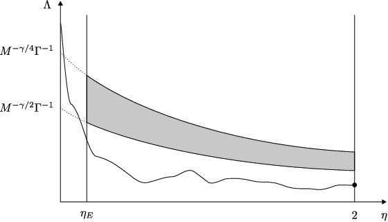
Now we explain Claim 1. We will work on the event , where we may invoke (2.56) to estimate and . In order to estimate , we expand the right-hand side of (2.53) in to get (2.54). Using (2.56) to estimate , we therefore have
| (2.66) |
We write the left-hand side as with the vector . Inverting the operator , we therefore conclude that
| (2.67) |
Together with (2.56) and , we therefore get
| (2.68) |
On the event we may estimate
Moreover, by definition of , we have . Using the definition of (2.18), we therefore get
Plugging this into (2.68) yields , which is Claim 1.
2.4.3 Sketch of the proof of Proposition 2.13
This argument is very similar to the proof of Claim 1 in Section 2.4.2. We can work on the event , then the bound (2.56) is available to estimate and . Next, we estimate . We expand the right-hand side of (2.53), we get
Using the fluctuation averaging estimate (2.75) explained in the next section, as well as (2.56), we find
| (2.70) |
which, combined with (2.56), yields
| (2.71) |
where in the last step we used the assumption and . ∎
2.4.4 Fluctuation averaging: proof of Proposition 2.14
The leading error in the self-consistent equation (2.54) for is . Among the three summands of , see (2.36), typically is the largest, thus we typically have
| (2.72) |
in the regime where is bounded. The large deviation bounds in Theorem 2.9 show that and a simple second moment calculation shows that this bound is essentially optimal. On the other hand, (2.29) shows that the typical size of the off-diagonal resolvent matrix elements is at least of order , thus the estimate
is essentially optimal in the standard Wigner case . Together with (2.72) this shows that the natural bound for is , which is also reflected in the bound (2.19).
However, the bound (2.20) for the average, , is of order , i.e. it is one order better than the bound for . For the purpose of , it is the average of the leading errors that matters, see (2.55). Since , the leading term in , is a fluctuating quantity with zero expectation, the improvement comes from the fact that fluctuations cancel out in the average. The basic example of this phenomenon is the central limit theorem. In our case, however, are not independent. In fact, their correlations do not decay, at least in the Wigner case where all indices play symmetric role. Thus standard results on central limit theorems for weakly correlated random variables do not apply.
Here we formulate a version of the fluctuation averaging mechanism, taken from [30], that is the most useful for this discussion and we comment on the history afterwards.
We shall perform the averaging with respect to a family of weights satisfying
| (2.73) |
Typical example weights are and . Note that in both of these cases commutes with .
Theorem 2.16 (Fluctuation averaging).
The first version of the fluctuation averaging mechanism appeared in [46] for the Wigner case, where was bounded by . Since is essentially , see (2.26), this corresponds to the first bound in (2.74). A different proof (with a better bound on the constants) was given in [47]. A conceptually streamlined version of the original proof was extended to sparse matrices [31] and to sample covariance matrices [73]. Finally, an extensive analysis in [29] treated the fluctuation averaging of general polynomials of resolvent entries and identified the order of cancellations depending on the algebraic structure of the polynomial. Moreover, in [29] an additional cancellation effect was found for the quantity . This improvement plays a key role in the proof of Theorem 2.10, see (2.42).
All proofs of the fluctuation averaging theorems rely on computing expectations of high moments of the averages and carefully estimating various terms of different combinatorial structure. In [29] we have developed a Feynman diagrammatic representation for bookkeeping the terms, but this is necessary only for the case of general polynomials. For the special cases stated in Theorem 2.16, the proof is relatively simple and it is presented in Appendix B of [30]. Here we will not repeat the proof, we only indicate the main mechanism by estimating the second moment of the first term in (2.74). The actual proof requires estimating all moments and then use Chebysev inequality to translate the moment estimates to probabilistic estimates standing behind the notation in (2.74).
Second moment calculation. First we claim that
| (2.76) |
Indeed, from Schur’s complement formula (2.26) we get . The first term is estimated by . The second term is estimated exactly as in (2.61) and (2.62), giving . In fact, the same bound (2.76) holds if is replaced with as long as is bounded.
Abbreviate and compute the variance
| (2.77) |
Using the bounds (2.73) on and (2.76), we find that the first term on the right-hand side of (2.77) is , where we used that is admissible. Let us therefore focus on the second term of (2.77). Using the fact that , we apply (2.27) to and to get
| (2.78) |
We multiply out the parentheses on the right-hand side. The crucial observation is that if the random variable is independent of (see Definition 2.7) then . Hence out of the four terms obtained from the right-hand side of (2.78), the only nonvanishing one is
where we used that the denominators are harmless, see (2.59). Together with (2.73), this concludes the proof of , which means that is bounded by in second moment sense. ∎
2.5 Remark on the proof of the local semicircle law with using the spectral gap
In Section 2.4 we proved the local semicircle law, Theorem 2.3, uniformly for instead of the larger regime . The difference between these two thresholds stems from the difference between and , see (2.17) and (2.48).
The bound on the norm of entered the proof when the self-consistent equation (2.66) was solved. The key idea is to solve the self-consistent equation (2.66) separately on the subspace of constants (the span of the vector ) and on its orthogonal complement . Roughly speaking, we obtain
| (2.79) |
instead of (2.67). In fact, we can improve this by using the fluctuation averaging. Subtracting the average over from the self-consistent equation (2.54) and estimating , we have
| (2.80) |
where in the last step we used the fluctuation averaging estimate (2.75) with , and from (2.56).
On the space of constant vectors, (2.53) becomes a scalar equation for the average , which can be expanded up to second order. More precisely, assuming , we can expand (2.53) up to second order:
| (2.81) |
In order to get a closed equation for , we take the average over :
| (2.82) |
The nonlinear term is estimated by
where (2.80) was used. The average can be estimated by as in Proposition 2.14. Moreover, is estimated by as in Lemma 2.15. We thus obtain a quadratic equation for the scalar quantity :
| (2.83) |
The main control parameter in this proof is , and the key iterative scheme is formulated in terms of . However, many intermediate estimates still involve . In particular, the self-consistent equation (2.53) is effective only in the regime where is already small and in the calculation above we tacitly used that . Hence we need a preparatory step to prove an apriori bound on , essentially showing that , in fact we will need (compare with Proposition 2.12). This proof itself is a continuity argument similar to the proof of Proposition 2.12; now, however, we have to follow and in tandem. The main reason why is already involved in this part is that we work in larger spectral domain , defined by using . Thus, already in this preparatory step, the self-consistent equation has to be solved separately on the subspace of constants and its orthogonal complement. We will omit here these details.
The second preparatory step is to control in terms of , which allows us to express the error terms in the self-consistent equation (2.83) in terms of . We first notice that (2.80) implies
i.e.
Using the apriori bound , we get
This equation is analogous to (2.51) and can be iterated as in the application of in Proposition 2.13 leading to (2.52) to obtain
| (2.84) |
Plugging this bound into (2.83), we have a self-consistent equation for the scalar quantity since . An elementary calculation, using the apriori bound , yields
| (2.85) |
Finally, in the main step we solve the quadratic inequality (2.85) for . If we neglect the error term in (2.85), then the equation reduces to
| (2.86) |
which has two solutions: either or . Away from the spectral edge we have with some positive constant , so the two solutions are separated and they both are stable under small perturbations. The second solution would mean that is strictly separated away from zero. But this can be excluded by a continuity argument: for large , say , it is easy to prove that is small. Since is a continuous function of , we find that as decreases continuously, cannot suddenly jump from a value near zero to a value near . Thus must remain in the vicinity of the zero solution to (2.86). This completes the sketch of the proof of Theorem 2.3 for the more general case . ∎
3 Universality of the correlation functions for Wigner matrices
In this section we explain the sketch of the proof of Theorem 1.2.
3.1 Dyson Brownian motion and the local relaxation flow
3.1.1 Concept and results
The Dyson Brownian motion (DBM) describes the evolution of the eigenvalues of a Wigner matrix as an interacting point process if each matrix element evolves according to independent (up to symmetry restriction) Brownian motions. We will slightly alter this definition by generating the dynamics of the matrix elements by an Ornstein-Uhlenbeck (OU) process which leaves the standard Gaussian distribution invariant. In the Hermitian case, the OU process for the rescaled matrix elements is given by the stochastic differential equation
| (3.1) |
where , , are independent complex Brownian motions with variance one and are real Brownian motions of the same variance. Denote the distribution of the eigenvalues of at time by where is given by (1.10) with the Gaussian potential .
Then satisfies [24]
| (3.2) |
where
| (3.3) |
The parameter is chosen as follows: for complex Hermitian matrices and for symmetric real matrices. Our formulation of the problem has already taken into account Dyson’s observation that the invariant measure for this dynamics is . A natural question regarding the DBM is how fast the dynamics reaches equilibrium. Dyson had already posed this question in 1962:
Dyson’s conjecture [24]: The global equilibrium of DBM is reached in time of order one and the local equilibrium (in the bulk) is reached in time of order . Dyson further remarked,
“The picture of the gas coming into equilibrium in two well-separated stages, with microscopic and macroscopic time scales, is suggested with the help of physical intuition. A rigorous proof that this picture is accurate would require a much deeper mathematical analysis.”
We will prove that Dyson’s conjecture is correct if the initial data of the flow is a Wigner ensemble, which was Dyson’s original interest. Our result in fact is valid for DBM with much more general initial data that we now survey. Briefly, it will turn out that the global equilibrium is indeed reached within a time of order one, but local equilibrium is achieved much faster if an a-priori estimate on the location of the eigenvalues (also called points) is satisfied. To formulate this estimate, let denote the location of the -th point under the semicircle law, i.e., is defined by (2.21).
A-priori Estimate: There exists an such that
| (3.4) |
with a constant uniformly in . This condition first appeared in [40].
The main result on the local ergodicity of Dyson Brownian motion states that if the a-priori estimate (3.4) is satisfied then the local correlation functions of the measure are the same as the corresponding ones for the Gaussian measure, , provided that is larger than . The -point correlation functions of the probability measure are defined, similarly to (1.4), by
| (3.5) |
Due to the convention that one can view the locations of eigenvalues as the coordinates of particles, we have used , instead of , in the last equation. From now on, we will use both conventions depending on which viewpoint we wish to emphasize. Notice that the probability distribution of the eigenvalues at the time , , is the same as that of the Gaussian divisible matrix:
| (3.6) |
where is the initial generalized Wigner matrix and is an independent standard GUE (or GOE) matrix. This establishes the universality of the Gaussian divisible ensembles. The precise statement is the following theorem:
Theorem 3.1.
We can choose depending on . In [41] explicit bounds on the speed of convergence and the optimal range of were also established. In particular, thanks to the optimal rigidity estimate (2.22) which implies that (3.4) holds with any , the range of the energy averaging in (3.7) can be reduced to , , but only for (Theorem 2.3 of [47]).
Theorem 3.1 is a consequence of the following theorem which identifies the averaged gap distribution of the eigenvalues.
Theorem 3.2 (Universality of the Dyson Brownian motion for short time).
[41, Theorem 4.1]
Suppose and
let be a smooth function with compact
support.
Then for
any sufficiently small , independent of , there exist
constants , depending only on and such that
for any
we have
| (3.8) |
In particular, if the a-priori estimate (3.4) holds with some and is of order , then for any the right hand side converges to zero as , i.e. the gap distributions for and coincide.
The test functions can be generalized to
| (3.9) |
for any fixed which is needed to identify higher order correlation functions. In applications, is chosen to be the indices of the eigenvalues in the interval and thus . This identifies the averaged gap distributions of eigenvalues and thus also identifies the correlation functions after energy averaging. We will not explain here in detail how to pass information from gap distribution to correlation functions (see Section 7 in [41]), but we note that this transfer is relatively easy if both statistics are averaged on a scale larger than the typical fluctuation of a single eigenvalue (which is smaller than in the bulk by (2.22)). This concludes Theorem 3.1. Note that the input of this theorem, the apriori estimate (3.4), identifies the location of the eigenvalues only on a scale which is much weaker than the precision for the eigenvalue differences in (3.8).
3.1.2 Main ideas behind the proof of Theorem 3.2
The key method is to analyze the relaxation to equilibrium of the dynamics (3.2). This approach was first introduced in Section 5.1 of [40]; the presentation here follows [41].
We start with a short review of the logarithmic Sobolev inequality for a general measure. Let the probability measure on be given by a general Hamiltonian :
| (3.10) |
In applications will be the Gaussian equilibrium measure, (1.10) with , so we use the same notation , but the statements in the beginning of this section hold for a general measure. Let be the generator, symmetric with respect to the measure , defined by the associated Dirichlet form
| (3.11) |
Recall the relative entropy of two probability measures:
If , then we will sometimes use the notation . The entropy can be used to control the total variation norm via the well known inequality
| (3.12) |
Let be the solution to the evolution equation
| (3.13) |
with a given initial condition . The evolution of the entropy satisfies
| (3.14) |
Following Bakry and Émery [6], the evolution of the Dirichlet form satisfies the inequality
| (3.15) |
If the Hamiltonian is convex, i.e.,
| (3.16) |
with some constant , then we have
| (3.17) |
Integrating (3.14) and (3.17) back from infinity to 0, we obtain the logarithmic Sobolev inequality (LSI)
| (3.18) |
and the exponential relaxation of the entropy and Dirichlet form on time scale
| (3.19) |
As a consequence of the logarithmic Sobolev inequality, we also have the concentration inequality for any and
| (3.20) |
We will not use this inequality in this section, but it will become important in Section 4.1.
Returning to the classical ensembles, we assume from now on that is given by (1.10) with and the equilibrium measure is the Gaussian one. We then have the convexity inequality
| (3.21) |
This guarantees that satisfies the LSI with and the relaxation time to equilibrium is of order one.
The key idea is that the relaxation time is in fact much shorter than order one for local observables that depend only on the eigenvalue differences. Equation (3.21) shows that the relaxation in the direction is much faster than order one provided that are close. However, this effect is hard to exploit directly due to that all modes of different wavelengths are coupled. Our idea is to add an auxiliary strongly convex potential to the Hamiltonian to “speed up” the convergence to local equilibrium. On the other hand, we will also show that the cost of this speeding up can be effectively controlled if the a-priori estimate (3.4) holds.
The auxiliary potential is defined by
| (3.22) |
i.e. it is a quadratic confinement on scale for each eigenvalue near its classical location, where the parameter will be chosen later. The total Hamiltonian is given by
| (3.23) |
where is the Gaussian Hamiltonian given by (1.10). The measure with Hamiltonian ,
| (3.24) |
will be called the local relaxation measure.
The local relaxation flow is defined to be the flow with the generator characterized by the natural Dirichlet form w.r.t. , explicitly, :
| (3.25) |
We will choose so that the additional term substantially increases the lower bound (3.16) on the Hessian, hence speeding up the dynamics so that the relaxation time is at most .
The idea of adding an artificial potential to speed up the convergence appears to be unnatural here. The current formulation is a streamlined version of a much more complicated approach that appeared in [40] and which took ideas from the earlier work [36]. Roughly speaking, in hydrodynamical limit, the short wavelength modes always have shorter relaxation times than the long wavelength modes. A direct implementation of this idea is extremely complicated due to the logarithmic interaction that couples short and long wavelength modes. Adding a strongly convex auxiliary potential shortens the relaxation time of the long wavelength modes, but it does not affect the short modes, i.e. the local statistics, which are our main interest. The analysis of the new system is much simpler since now the relaxation is faster, uniform for all modes. Finally, we need to compare the local statistics of the original system with those of the modified one. It turns out that the difference is governed by which can be directly controlled by the a-priori estimate (3.4).
Our method for enhancing the convexity of is reminiscent of a standard convexification idea concerning metastable states. To explain the similarity, consider a particle near one of the local minima of a double well potential separated by a local maximum, or energy barrier. Although the potential is not convex globally, one may still study a reference problem defined by convexifying the potential along with the well in which the particle initially resides. Before the particle reaches the energy barrier, there is no difference between these two problems. Thus questions concerning time scales shorter than the typical escape time can be conveniently answered by considering the convexified problem; in particular the escape time in the metastability problem itself can be estimated by using convex analysis. Our DBM problem is already convex, but not sufficiently convex. The modification by adding enhances convexity without altering the local statistics. This is similar to the convexification in the metastability problem which does not alter events before the escape time.
3.1.3 Some details on the proof of Theorem 3.2
The core of the proof is divided into three theorems. For the flow with generator , we have the following estimates on the entropy and Dirichlet form.
Theorem 3.3.
Consider the forward equation
| (3.26) |
with the reversible measure defined in (3.24). The initial condition satisfies . Then we have the following estimates
| (3.27) |
| (3.28) |
and the logarithmic Sobolev inequality
| (3.29) |
with a universal constant . Thus the relaxation time to equilibrium is of order :
| (3.30) |
Proof.
Notice that the estimate (3.28) is an additional information that we extracted from the Bakry-Émery argument by using the second term in the Hessian estimate (3.21). It plays a key role in the next theorem.
Theorem 3.4 (Dirichlet form inequality).
Let be a probability density and let be a smooth function with compact support. Then for any and any we have
| (3.33) |
Proof. For simplicity, we assume that . Let satisfy
with an initial condition . We write
| (3.34) | ||||
The second term in (3.34) can be estimated by (3.12), the decay of the entropy (3.30) and the boundedness of ; this gives the second term in (3.33).
To estimate the first term in (3.34), by the evolution equation and the definition of we have
From the Schwarz inequality and , the last term is bounded by
| (3.35) | ||||
where we have used (3.28) and that due to being smooth and compactly supported. ∎
Alternatively, we could have directly estimated the left hand side of (3.33) by using the total variation norm between and , which in turn could be estimated by the entropy (3.12) and the Dirichlet form using the logarithmic Sobolev inequality, i.e., by
| (3.36) |
However, compared with this simple bound, the estimate (3.33) gains an extra factor in the denominator, i.e. it is in terms of Dirichlet form per particle. The improvement is due to the fact that the observable in (3.33) depends only on the gap, i.e. difference of points. This allows us to exploit the additional term (3.28) gained in the Bakry-Émery argument. This is a manifestation of the general observation that gap-observables behave much better than point-observables.
The final ingredient in proving Theorem 3.2 is the following entropy and Dirichlet form estimates.
Theorem 3.5.
Suppose that (3.21) holds. Let be fixed and recall the definition of from (3.4). Fix a constant and consider the local relaxation measure with this . Set and let . Suppose there is a constant such that
| (3.37) |
Then for any the entropy and the Dirichlet form satisfy the estimates:
| (3.38) |
where the constants depend on and .
Proof. The evolution of the entropy can be computed explicitly by the formula [87]
Hence we have, by using (3.25),
Since is -invariant and time independent, the middle term on the right hand side vanishes, and from the Schwarz inequality
| (3.39) |
Notice that (3.39) is reminiscent to (3.14) for the derivative of the entropy of the measure with respect to . The difference is, however, that does not satisfy the evolution equation with the generator . The last term in (3.39) expresses the error.
Together with the logarithmic Sobolev inequality (3.29), we have
| (3.40) |
Integrating the last inequality from to and using the assumption (3.37) and , we have proved the first inequality of (3.38). Using this result and integrating (3.39), we have
By the convexity of the Hamiltonian, is decreasing in . Since , this proves the second inequality of (3.38). ∎
Finally, we complete the proof of Theorem 3.2. For any given we now choose and we construct the local relaxation measure with this . Set and let be the density in Theorem 3.4. Then Theorem 3.5, Theorem 3.4 and an easy bound on the entropy imply that
| (3.41) |
i.e., the local statistics of and are the same for any initial data for which (3.37) is satisfied. Applying the same argument to the Gaussian initial data, , we can also compare and . We have thus proved (3.8) and hence the universality. ∎
3.2 The Green function comparison theorems and four moment matching
We now state the Green function comparison theorem, Theorem 3.6. It will quickly lead to Theorem 3.7 stating that the correlation functions of eigenvalues of two matrix ensembles are identical on a scale smaller than provided that the first four moments of all matrix elements of these two ensembles are almost the same. We will state a limited version for real Wigner matrices for simplicity of presentation.
Theorem 3.6 (Green function comparison).
[45, Theorem 2.3] Suppose that we have two Wigner matrices, and , with matrix elements given by the random variables and , respectively, with and satisfying the uniform subexponential decay condition (1.17). We assume that the first four moments of and are close to each other in the sense that
| (3.42) |
holds for some . Then there are positive constants and , depending on and from (1.17) such that for any with and for any with , , we have
| (3.43) |
where and denotes the Green functions of and .
Here we formulated Theorem 3.6 for a product of two traces of the Green function, but the result holds for a large class of smooth functions depending on several individual matrix elements of the Green functions as well, see [45] for the precise statement. (The matching condition (3.42) is slightly weaker than in [45], but the proof in [45] without any change yields this slightly stronger version.) This general version of Theorem 3.6 implies the correlation functions of the two ensembles at the scale are identical:
Theorem 3.7 (Correlation function comparison).
Notice that these comparison theorems hold for any fixed energy , i.e. no averaging in energy is necessary.
The basic idea for proving Theorem 3.6 is similar to Lindeberg’s proof of the central limit theorem, where the random variables are replaced one by one with a Gaussian one. We will replace the matrix elements with one by one and estimate the effect of this change on the resolvent by a resolvent expansion. The idea of applying Lindeberg’s method in random matrices was recently used by Chatterjee [15] for comparing the traces of the Green functions; the idea was also used by Tao and Vu [81] in the context of comparing individual eigenvalue distributions.
The four moment matching condition (3.42) with first appeared in [81]. For comparison with Theorem 3.6, we state here the main result of [81]. Let and denote the eigenvalues of and , respectively. Then the joint distribution of any -tuple of eigenvalues on scale is very close to each other in the following sense:
Theorem 3.8 (Four moment theorem for eigenvalues).
[81, Theorem 15] Let and be two Wigner matrices. Assume that the first four moments of and exactly match and the subexponential decay (1.17) holds for the single entry distributions. Then for any sufficiently small positive and and for any function satisfying , , and for any selection of -tuple of indices away from the edge, we have
| (3.45) |
with some . The exact moment matching condition can be relaxed to (3.42), but will depend on .
Note that the arguments in (3.45) are magnified by a factor so the result is sufficiently precise to detect individual eigenvalue correlations. Therefore Theorem 3.6 or 3.8 can prove bulk universality for a Wigner matrix if another is found, with matching four moments, for which universality is already proved. This will be explained in Section 3.3.
Both Theorem 3.6 and Theorem 3.8 rely on some version of the local semicircle law on the shortest possible scale. There are, however, three main differences between them.
- (i)
- (ii)
Both theorems are of perturbative nature that require some apriori information. Theorem 3.6 uses a bound on the resolvent matrix entries, , that has already been obtained in the local semicircle law (see, e.g. (2.19)). Theorem 3.8 needs an apriori lower bound on the gaps to exclude possible eigenvalue resonances that may render the expansion unstable. This is achieved by a level repulsion estimate that is the most complicated technical part of [81]. Previously, even more precise level repulsion estimates were obtained in [39] but only for smooth distributions.
- (iii)
Theorem 3.6 also compares off-diagonal Green function elements, an information that cannot be obtained from Theorem 3.8. Hence it directly provides information on the eigenvectors as well, see [58] for the development. In fact, once Theorem 3.6 is proved for all energies, it also implies Theorem 3.8. The reason is that we can integrate correlation functions in energy with a precision smaller than the typical size of the gap, hence eigenvalues with a fixed label can be identified. This was first done near the edge in [32] and later in the bulk in [58].
Sketch of the proof of Theorem 3.6. We fix a bijective ordering map on the index set of the independent matrix elements,
and denote by the Wigner matrix whose matrix elements follow the -distribution if and they follow the -distribution otherwise; in particular and .
Consider the telescopic sum of differences of expectations (we present only one resolvent for simplicity of the presentation):
| (3.46) | ||||
Let denote the matrix whose matrix elements are zero everywhere except at the position, where it is 1, i.e., . Fix a and let be determined by . We will compare with . Note that these two matrices differ only in the and matrix elements and they can be written as
with a matrix that has zero matrix element at the and positions.
By the resolvent expansion,
and a similar expression holds for the resolvent of by . From the local semicircle law for individual matrix elements (2.19), the matrix elements of all Green functions , are bounded by . Although (2.19) is not directly applicable to , it is easy to show that
so choosing we can prove a bound for slightly below at the expense of a factor . The estimates of the related resolvents , are similar.
By assumption (3.42), the difference between the expectation of matrix elements of and is of order . Since the number of steps, is of order , the difference in (3.46) is of order , and this proves Theorem 3.6 for a single resolvent. It is very simple to turn this heuristic argument into a rigorous proof and to generalize it to the product of several resolvents. The real difficulty is the input that the resolvent entries can be bounded for a general class of Wigner matrices down to the almost optimal scale .
3.3 Universality for generalized Wigner matrices: putting it together
In this short section we put the previous information together to prove Theorem 1.2. We first focus on the case when is independent of . Recall that Theorem 3.1 states that the correlation functions of the Gaussian divisible ensemble,
| (3.47) |
where is the initial Wigner matrix and is an independent standard GUE (or GOE) matrix, are given by the corresponding GUE (or GOE) for provided that the a-priori estimate (3.4) holds for the solution of the forward equation (3.2) with some exponent . Since the rigidity of eigenvalues (2.22) holds uniformly for all generalized Wigner matrices, we have proved (3.4) for with any .
From the evolution of the OU process (3.1) for we have
| (3.48) |
for and with the choice of . Furthermore, are independent of for due to and . Hence (3.42) is satisfied for the matrix elements of and and we can thus use Theorem 3.7 to conclude that the correlation functions of and are identical at the scale . Since the correlation functions of are given by the corresponding Gaussian case, we have proved Theorem 1.2 under the condition that the probability distribution of the matrix elements decay subexponentially. Finally, we need a technical cutoff argument to relax the decay condition to (1.13) which we omit here (see Section 7 in [32]).
The argument for -dependent in the range , , is slightly different. For such a small , (3.7) could be established only for relatively large times, . We cannot therefore compare with directly, since the deviation of the third moments of and in (3.48) would not satisfy (3.42). Instead, we construct an auxiliary Wigner matrix such that up to the third moment its time evolution under the OU flow (3.47) matches exactly the original matrix and the fourth moments are close even for of order (see Lemma 3.4 of [46]). Theorem 3.1 will then be applied for , and Theorem 3.6 can be used to compare and . This completes the sketch of the proof of Theorem 1.2.
4 Universality of the correlation functions for -ensembles
In this section we outline the proof of Theorem 1.4. We will use the notation for the probability measure defining the general -ensemble with a potential on ordered real points , see (1.10). We let and denote the probability and the expectation with respect to . The equilibrium density is denoted by and its Stieltjes transform by
The classical location of the -th point will be denoted by , see (1.22). Note that in this section , , and refer to the quantities related to the general and not the Gaussian one as in the previous sections. This avoids carrying the subscripts all the time as in Section 2 we dropped the subscripts sc referring to the semicircle law.
4.1 Rigidity estimates
For simplicity of presentation we assume that the potential is convex, i.e.,
| (4.1) |
the equilibrium density is supported on a single interval and satisfies (1.20) (for the general case, see [12]). The Gaussian case corresponds to , in which case the equilibrium density is the semicircle law, , given by (1.3). Our main result concerning the universality is Theorem 1.4 and similar statement holds for the universality of the averaged gap distributions directly. In fact, the proof of Theorem 1.4 goes via the averaged gap distribution as we now explain.
The first step to prove Theorem 1.4 is the following theorem which provides a rigidity estimate on the location of each individual point. The precision in the bulk is almost down to the optimal scale , the estimate is weaker near the edges. In the following, we will denote .
Theorem 4.1.
We explain some ideas of the proof of (4.2), the arguments for (4.3) are similar and (4.4) follows from an easy large deviation bound, see [11]. The first ingredient to prove (4.2) is an analysis of the loop equation following Johansson [57] and Shcherbina [78]. The equilibrium density , for a convex potential , is given by
| (4.5) |
where is a real function that can be extended to an analytic function in and has no zero in . Denote by where the square root is defined such that its asymptotic value is as . Recall that the density is the one-point correlation function which is characterized by
| (4.6) |
Let and be the Stieltjes transforms of the density and the equilibrium density , respectively. Notice that in Section 2 we have used to denote the Stieltjes transform of the empirical measure (2.11); here denotes the ensemble average of the analogous quantity.
Define the analytic functions
and
Here for complex random variables we use the definition that .
The equation used by Johansson (which can be obtained by a change of variables in (4.6) [57] or by integration by parts [78]), is a variation of the loop equation (see, e.g., [48]) used in the physics literature and it takes the form
| (4.7) |
Equation (4.7) can be used to express the difference in terms of , and . In the regime where is small, we can neglect the quadratic term. The term is of the same order as and is difficult to treat. As observed in [5, 78], for analytic , this term vanishes when we perform a contour integration. So we have roughly the relation
| (4.8) |
where we dropped the less important error involving due to the extra factor. In the convex setting, the variance can be estimated by the logarithmic Sobolev inequality and we immediately obtain an estimate on . We then use the Helffer-Sjöstrand formula, see (2.24), to estimate the locations of the particles. This will provide us with an accuracy of order for . This argument gives only an estimate on the expectation of the locations of the particles since we only have information on the averaged quantity, . Although it is tempting to use this new accuracy information on the particles to estimate the variance again in (4.8), the information on the expectation on alone is very difficult to use in a bootstrap argument. To estimate the variance of a non-trivial function of we need high probability estimates on .
The key idea in this section is the observation that the accuracy information on the ’s can be used to improve the local convexity of the measure in the direction involving the differences of ’s. To explain this idea, we compute the Hessian of the Hamiltonian of :
The naive lower bound on is , but for a typical it is in fact much better in most directions. To see this effect, suppose we know with some for any , where . Then for with we have
| (4.9) |
This improves the convexity of the Hessian to on the hyperplane . Let
denote the block average of the locations of particles and rewrite
as a telescopic sum with an appropriate sequence of , with the property that . We can now use the improved concentration on the hyperplane to the variables to control the fluctuation of . Since the fluctuation of is very small for small , we finally arrive at the estimate
| (4.10) |
From (4.10) we thus have that with high probability. This improves the starting accuracy for to with some , provided that we can prove that . But the last inequality involves only expectations and it will follow from the analysis of the loop equation (4.7) we just mentioned above. Starting from , this procedure can be repeated by decreasing step by step until we get the optimal accuracy, . The implementation of this argument in [11] is somewhat different from this sketch due to various technical issues, but it follows the same basic idea.
4.2 The local equilibrium measure
Having completed the first step, the rigidity estimate, we now focus on the second step, i.e. on the uniqueness of the local Gibbs measure. Let . Choose and set (the integer part). Fix an integer with . We will study the local spacing statistics of consecutive particles
These particles are typically located near determined by the relation
Note that .
We will distinguish the inside and outside particles by renaming them as
| (4.11) |
but note that they keep their original indices. The notation refers to the simplex in . In short we will write
all in increasing order, i.e. and . We will refer to the ’s as external points and to the ’s as internal points.
We will fix the external points (also called as boundary conditions) and study conditional measures on the internal points. We define the local equilibrium measure on with fixed boundary condition by
| (4.12) |
Note that for any fixed , the measure is supported on configurations of points located in the interval .
The Hamiltonian of the measure is given by
| (4.13) |
We now define the set of good boundary configurations with a parameter
| (4.14) |
where is a small constant to cutoff points near the spectral edges. Some rather weak additional conditions for near the spectral edges will also be needed. They can be built in the definition of based upon the bounds (4.3) and (4.4) but we will neglect this issue here.
Let and be two measures of the form (1.10) with potentials and and densities and , respectively. For our purpose , i.e., is the Gaussian -ensemble and its density is the Wigner semicircle law. Let the sequence be the classical locations for and the sequence be the classical locations for . Similarly to the construction of the measure , for any positive integer we can construct the measure conditioned that the particles outside are given by the classical locations for . More precisely, we define a reference local Gaussian measure on the set via the Hamiltonian
| (4.15) |
where . Since will not play an active role, we will abuse the notation and set .
The measure lives on the interval while the measure lives on the interval and it is difficult to compare them. But after an appropriate translation and dilation, they will live on the same interval and from now on we assume that . The parameter has to be sufficiently small since and are not constant functions and we have to match these two densities quite precisely in the whole interval. There are some other subtle issues related to the rescaling, but we will neglect them here to concentrate on the main ideas. Our main result is the following theorem which is essentially a combination of Proposition 4.2 and Theorem 4.4 from [11].
Theorem 4.2.
Let . Fix , and . Then for we have
| (4.16) |
as for any smooth and compactly supported test function . A similar formula holds for more complicated observables of the form (3.9).
From the rigidity estimate, Theorem 4.1, it follows that has an overwhelming probability, so the expectation can be changed to and similarly for the reference measure. Once (4.16) is proven for all observables of the form (3.9), we get that the locally averaged gap statistics for coincide with those of the reference Gaussian case, hence they are universal. Since averaged gap statistics identifies locally averaged correlation functions, we obtain Theorem 1.4.
It remains to prove Theorem 4.2. The basic idea is to use the Dirichlet form inequality (3.33). Although (3.33) was stated for an infinite volume measure, it holds for any measure with repulsive logarithmic interactions in a finite volume and with the parameter being the lower bound on the Hessian of the Hamiltonian. In our setting, we denote by the lower bound for , and the Dirichlet form inequality becomes
| (4.17) |
where
| (4.18) |
Thus our task is to prove that
| (4.19) |
By definition,
where is defined as
| (4.20) |
Using the equilibrium relation (1.20) between the potentials , and the densities , , we have
Hence is the sum of the error terms,
| (4.21) | ||||
| (4.22) |
and there is a term similar to with replaced by and replaced by .
With our convention, the total numbers of particles in the interval are equal and thus
Since the densities and are functions away from the endpoints and and is small, is small in the interval and thus is small. For estimating , we can replace the integral
with negligible errors, at least for ’s away from the edges, . Thus
| (4.23) |
and can be estimated by the assumption from . The same argument works if is close to the edge, but is away from the edges, i.e. or . The edge terms, for , are difficult to estimate due to the singularity in the denominator and the event that many ’s with may pile up near . To resolve this difficulty, we show that the averaged local statistics of the measure are insensitive to the change of the boundary conditions for near the edges. This can be achieved by the simple inequality
| (4.24) |
for any two boundary conditions and . Although we still have to estimate the entropy that includes a logarithmic singularity, this can be done much more easily since entropy is less sensitive to singularities than Dirichlet form. Therefore, we can replace the boundary condition with for and then the most singular edge terms in (4.20) cancel out.
We note that we can perform this replacement only for a small number of index pairs , since estimating the gap distribution by the total entropy, as noted in (3.36) in Section 3.1, is not as efficient as the estimate using the Dirichlet form per particle. Thus we can afford to use this argument only for the edge terms, . For all other index pairs we still have to estimate by exploiting that is a good configuration, i.e. is small.
Unfortunately, even with the optimal accuracy in (4.14) as an input, the relation (4.19) still cannot be satisfied for any choice of . To understand this problem, we remark that while the edge terms become a smaller percentage of the total terms in (4.24) as gets bigger, the relaxation time to equilibrium for , determined by the convexity of , increases at the same time. At the end of our calculation, there is no good regime for the choice of . Fortunately, this can be resolved by using the idea of the local relaxation measure as in (3.22), i.e., we add a quadratic term to the Hamiltonian of the measure and for the measure . With these ideas, we can complete the proof of Theorem 4.2.
5 Single gap universality
In this section we outline the proofs of Theorem 1.3 and 1.5 following closely [44]. Both proofs rely on the single gap universality for the locally conditioned measure introduced already in (4.12). This will be stated in Theorem 5.1, whose proof takes up most of this section. At the end, in Section 5.4 we complete the proofs of Theorem 1.3 and 1.5.
5.1 Statements on local equilibrium measures
5.1.1 Definition
We work in the bulk spectrum and we consider the local equilibrium measure on points which is the conditional measure after fixing all other points. To define it precisely, we fix two small positive numbers, and choose two positive integer parameters such that
| (5.1) |
All results will hold for any sufficiently small and for any sufficiently large , where the threshold depends on and maybe on other parameters of the model.
Denote the set of consecutive indices in the bulk. As in Section 4.2, we will distinguish external and internal points by renaming them as
| (5.2) |
the only difference is that here the internal particles are labelled symmetrically to . This discrepancy is only notational, but we prefer to follow the notations of the original papers. In short we will write
As in (4.12) we again define the local equilibrium measure on with boundary condition by
| (5.3) |
where is the (global) equilibrium measure (1.10). For a fixed , this measure can also be written as a Gibbs measure,
| (5.4) |
with Hamiltonian
| (5.5) |
Here can be viewed as the external potential of a -log-gas of the points in the configuration interval
5.1.2 Universality of the local gap statistics for
Our main technical result, Theorem 5.1 below, asserts that the local gap statistics is essentially independent of and as long as the boundary conditions are regular. This property is expressed by defining the following set of “good” boundary conditions with some given positive parameters (thet set in (4.14) played exactly the same role)
| (5.6) | ||||
This definition is taylored to the rigidity bounds for the -ensemble, see Theorem 4.1. Note that has a key parameter, the exponent , which will be chosen as an arbitrary small positive number in the applications. We will not follow its dependence precisely and we will often neglect it from the notation, i.e. we will talk about “good” boundary conditions .
Good boundary conditions give rise to a regular potential . More precisely, if , then
| (5.7) | ||||
| (5.8) | ||||
| (5.9) |
Here
denotes the midpoint of the configuration interval, is the distance of to the boundary of the configuration interval and and are regularized versions of the distances of to the closest and to the farthest endpoints of , respectively. The key point is that the leading term of depends on the boundary conditions only through the density in the center, . We also introduce
| (5.10) |
to denote the equidistant points within the interval .
Theorem 5.1 (Gap universality for local measures).
Fix and satisfying (5.1) with an exponent . Consider two boundary conditions such that the configuration intervals coincide,
| (5.11) |
We consider the measures and defined as in (5.4), with possibly two different external potentials and . Let be a small constant. Assume that satisfies
| (5.12) |
Suppose that and that
| (5.13) |
holds. Let the integer number satisfy for some small . Then there exists , depending on , such that if then for any fixed and any bounded smooth observable with compact support we have
| (5.14) | ||||
for some depending on and for some depending on . This holds for any sufficiently large, where depends on the parameters , and in (5.13).
5.1.3 Rigidity and level repulsion of
In the following two theorems we establish rigidity and level repulsion estimates for the local log-gas with good boundary conditions . While both rigidity and level repulsion are basic questions for log gases and are interesting in themselves, our main motivation to prove these theorems is to use them in the proof of Theorem 5.1.
We remark that an almost optimal rigidity estimate in the bulk was given in Theorem 4.1 and some level repulsion bound was given in (4.11) of [11], these results hold with respect to the global measure . For the proof of Theorem 5.1 we need their local versions with respect to , at least for most . Naively, this looks as a simple conditioning argument, but there is a subtle point. From the estimates w.r.t. , one can conclude that has a good rigidity bound for a set of boundary conditions with high probability w.r.t. the global measure . This will be sufficient for the proof of Theorem 1.5, but not for Theorem 1.3. In the proof for the gap universality of Wigner matrices we will need a rigidity estimate for for a set of ’s with high probability with respect to by the time evolved measure which may be asymptotically singular to for large . The following result asserts that a rigidity estimate holds for provided that itself satisfies a rigidity bound and an extra condition, (5.15), holds. This condition will have to be verified with different methods in the Wigner case.
Theorem 5.2 (Rigidity estimate for local measures).
For consider the local equilibrium measure defined in (5.4) and assume that
| (5.15) |
is satisfied. Then there are positive constants , depending on , such that for any and ,
| (5.16) |
The proof of this result is similar to that of the concentration estimate (4.10) in Theorem 4.1. To estimate , we again use a multiscale argument of local averages for which stronger convexity bounds are available. The analogue of the accuracy estimate controlling in Theorem 4.1 is replaced by the assumption (5.15). Notice that, unlike for the global measure , a direct accuracy control via the loop equation is not available for since the potential is not analytic.
Now we state the level repulsion estimates.
Theorem 5.3 (Level repulsion estimate for local measures).
For we have the following estimates:
i) [Weak form of level repulsion] For any we have
| (5.17) |
ii) [Strong form of level repulsion] Suppose that there exist positive constants such that the following rigidity estimate holds for any :
| (5.18) |
Then there exists small a constant , depending on in (5.18), such that for any . we have
| (5.19) |
The level repulsion bounds will mostly be used in the following estimate which trivially follows from Theorem 5.3
Corollary 5.4.
Let , then for any we have
| (5.20) |
∎
5.1.4 Sketch of the proof of the level repulsion
The proof of part (ii) of Theorem 5.3 goes in three steps. For simplicity, we consider (5.19) only for the first gap, i.e. and we also assume that by a simple shift.
Step 1. In this step we prove
| (5.21) |
which is essentially (5.19) but with factor instead of and with the exponent replaced with one. The proof of (5.21) is dilation argument. For a nonnegative parameter , we define
| (5.22) |
where we set
Clearly is the normalization constant of the measure and we have
| (5.23) |
The multiple integral on the r.h.s of (5.22) is almost the same as , except that the argument of is rescaled by . This effect can be estimated from the explicit formula (5.5) for . The external potential in (5.5) is unproblematic since it is smooth. Due to , the points are regularly spaced on scales at least , thus the sum of the interaction terms for ’s away from the edges of , i.e. or , is a regular function of and the effect of dilation can be well approximated by Taylor expansion. For nearby ’s right below the lower edge, i.e. , we use the trivial bound . From these estimates it follows that
| (5.24) |
Step 2. Now we consider an auxiliary measure which are slightly modified version of the local equilibrium measures:
| (5.25) |
where are chosen for normalization. In other words, we drop the term from the measure . Setting for brevity, we have
| (5.26) |
The estimate (5.21) also holds for and thus
and with the choice in (5.21) we also have
with some positive constant . This implies that
Combining with (5.26), we have thus proved that
| (5.27) |
i.e. we obtained (5.21) but with an exponent in the r.h.s.
Step 3. We now improve the constant to in the r.h.s of (5.21). The factor originated from the number of particles in . We can further condition the measure on the points
and we let denote the conditional measure on the remaining variables . From the rigidity estimate (5.18) we have with a very high probability w.r.t. . We will now apply (5.27) to the measure to obtain
| (5.28) |
This holds for all with a high -probability. The subexponential lower bound on , assumed in part ii) of Theorem 5.3, allows us to include the probability of the complement of in the estimate, we thus have proved (5.19).
The proofs of the weaker bound (5.17) for any use similar arguments that have led to (5.21), but without assuming which yields that one factor of has to be replaced with in (5.24). The assumption that the boundary conditions are good needs to be dropped since in Step 3 of the above argument, (5.21) is also used after additional conditioning on , distributed according to , and without (5.18) there is no rigidity result available for .
5.2 Proof of Theorem 5.1
In this section, we start to compare gap distributions of two local log-gases on the same configuration interval but with different external potential and boundary conditions. For simplicity, we consider only an observable of a single gap; a few consecutive gaps can be handled similarly. From now on, we use microscopic coordinates, i.e. we replace with , and we also relabel the indices so that the coordinates of are . This will have the advantage that remains the only large parameter; disappears.
The local equilibrium measures and their Hamiltonians will be denoted by the same symbols, and , as before, but with a slight abuse of notations we redefine them now to the microscopic scaling, i.e.
| (5.29) |
The other Hamiltonian is defined in a similar way with in (5.29) replaced with another external potential . We also rewrite (5.13) in the microscopic coordinate as
| (5.30) |
where is the rescaled version of the definition given in (5.10), but we keep the same notation. The concept of “good” set is also rescaled accordingly.
Suppose that and define the interpolating measures
| (5.31) |
so that and ( is a normalization constant). This is again a local log-gas with Hamiltonian
| (5.32) |
For any fixed , the measure inherits all relevant properties of . In particular the rigidity bound in the form
| (5.33) |
the level repulsion bounds (5.17)–(5.19) and their consequence in (5.20) hold w.r.t. the measure as well (in the new microscopic coordinates there are no factors in the left hand sides of these inequalities). The proofs are basically parallel with the arguments for ; the only nontrivial step is to show that (5.30) implies the analogous bound
w.r.t. as well. Although appears to be some easy combination of and , this conclusion is nontrivial. It requires comparing and via the entropy inequality, which involves controlling the exponential moment of w.r.t. . At this point the Gaussian tail proven in (5.16) is necessary.
The right hand side of (5.14) with , in the rescaled coordinates and with , is estimated by
| (5.34) |
For any bounded smooth function with compact support
| (5.35) |
where
| (5.36) |
and denotes the covariance. Thus Theorem 5.1 follows immediately from the following estimate on the gap covariance function. ∎
Theorem 5.5.
Consider two smooth potentials and two good boundary conditions, , such that the configuration intervals coincide, . For any let be the interpolating measure defined in (5.31). Assume that (5.30) holds for both boundary conditions . Fix . Then there exist and , depending on , such that for any sufficiently small , for we have
| (5.37) |
for any smooth function with compact support provided that is large enough.
Theorem 5.5 is our key technical result. The main difficulty behind it is due to the fact that the covariance function of two points, , decays only logarithmically. In fact, for the GUE, Gustavsson proved that (Theorem 1.3 in [54])
| (5.38) |
and a similar formula is expected for . Although depends strongly only on points near the boundary and is away from the boundary, it is still very difficult to prove Theorem 5.5 based on this slow logarithmic decay. However, the covariance function of the type
| (5.39) |
decays much faster in . Since the second factor depends only on the difference of two neighboring points, it is expected that the decay is the (discrete) derivative in of the covariance (5.38), i.e. it is . The actual result (5.37) is much weaker, but it still provides a power-law decay in instead of a logarithmic decay. Covariances of the form are expected to decay even faster but we have not pursued this direction further.
5.3 Decay of correlation functions: Proof of Theorem 5.5
We will express the difference of gap distributions between two measures in terms of random walks in time dependent random environments. The decay of correlation functions will be translated into a partial regularity property of the corresponding parabolic equation. This partial regularity is a discrete version of the De Giorgi-Nash-Moser theory but with a long range elliptic part.
5.3.1 Random Walk Representation
In this section we derive a random walk representation for the gap correlation function on the left hand side of (5.37). We will apply it for the interpolating measure (5.31) and for the function given in (5.36), but the representation formula (Proposition 5.6 below) is valid for any and .
Let be the reversible generator given by the Dirichlet form
| (5.40) |
This process can also be characterized by the following SDE
| (5.41) |
where is a family of independent standard real Brownian motions. Let denote the expectation for this process with initial point . The expectation with respect to the process starting from equilibrium is . With a slight abuse of notations, when we talk about the process, we will use and also to denote the probability and expectation w.r.t. this dynamics with initial data distributed w.r.t. , i.e., in equilibrium.
Suppose is the solution of the equation with an initial condition . Introduce the notation
| (5.42) |
By integrating the time derivative of and using the equation satisfies, we have
| (5.43) |
For any fixed , the inner integral on the right hand side can be expressed by a random walk representation. Fix a path . Define the following operators on
| (5.44) |
| (5.45) |
Clearly is diffusion operator with random rates and is a potential representing a random environment. These operators depend on the whole path , but we omit this fact from the notation.
With these notations we have the following representation:
Proposition 5.6.
For any smooth function , for any , , we have
| (5.46) |
Here, for any and for any fixed path we let denote the solution of the evolution equation
| (5.47) |
with initial data .
This representation in a slightly different setting already appeared in Proposition 2.2 of [16] (see also Proposition 3.1 in [53]), which was a probabilistic formulation of the idea of Helffer and Sjöstrand [55] and Naddaf and Spencer [69]. The proof relies on taking the gradient of the equation . A direct computation of the commutator yields that
| (5.48) |
with initial condition . Here , where is the operator given by the matrix in (5.45) and is the diagonal multiplication operator by . Since generates the process , we can represent the solution to (5.48) by the Feynman-Kac formula which can be written in the form (5.46).
When applying this proposition to our case, we will choose the initial condition be given by (5.36). The initial condition for the random walk (5.47) is given by . Notice that the leading term in cancel; this is because the leading term in (5.8) depends only on the density which is matched for and by , see (5.7). We thus have
| (5.49) |
i.e. initially is small away from the boundary and for the small regime the inner integral in the r.h.s. of (5.46) is small. After very long time becomes constant, but then the right hand side of (5.46) is zero. The analysis of (5.46) requires to monitor what happens to for coordinates away from the boundary at intermediate times.
5.3.2 Preparation for the De Giorgi-Nash-Moser bound: Restriction to the good paths
The representation (5.46) expresses the covariance function in terms of the discrete spatial derivative of the solution to (5.47). To estimate in (5.46), we will now study the Hölder continuity of the solution to (5.47) at time and at the spatial point . We will do it for each fixed path , with the exception of a set of “bad” paths that will have a small probability.
Notice that if all points were approximately regularly spaced in the interval , then the operator had a kernel , i.e. it were essentially a discrete version of the operator (in one dimension). Hölder continuity will thus be the consequence of the De Giorgi-Nash-Moser bound for the parabolic equation (5.47). However, we need to control the coefficients in this equation, which depend on the random walk .
For the De Giorgi-Nash-Moser theory we need both upper and lower bounds on the time dependent kernel . The rigidity bound (5.33) guarantees a lower bound on , up to a factor . Since the subexponential probabilistic estimate in (5.33) is very strong, one can easily guarantee a very similar estimate uniformly in time, i.e.
| (5.50) |
(maybe after reducing from (5.33)). This follows from the fact that is invariant under the dynamics and has some stochastic continuity.
The level repulsion estimate implies certain upper bounds on , but these estimates not particularly strong. Even in the case, the bound (5.20) implies only that
is finite. In the borderline case even the expectation of is infinite. Such a weak control does not allow us to guarantee an effective simultaneous bound on for all and for all time. Instead of supremum bounds, we control these coefficients only in an average sense and we can show that for any fixed index , time and parameter , we have
| (5.51) |
Here will be chosen as large constant times . The summation over is harmless since for the rigidity estimate can be used to bound . By a dyadic choice of the parameters , it is easy to upgrade (5.51) to hold for any and . But it is essential that a reference point be fixed, one cannot guarantee that none of the gaps closes.
The expectation over the paths, , in (5.46) will be restricted to the sets given in (5.50) and (5.51). Due to the strong subexponential bound, the restriction to the set in (5.50) is unproblematic. However, the estimate (5.51) is quite weak; the probability of the ”bad” paths is bounded only by a small negative power of . This is not sufficient to compensate the time integration in (5.46) even after the upper cutoff . We will need to use that the heat kernel of the equation (5.47) has an decay of order after time . Thus the solution decays as which renders the integration in (5.46) harmless.
For completeness, we state the heat kernel decay estimate in a general form. Notice that we only assume a lower bound in to guarantee sufficient ellipticity; there is no upper bound required for these bounds.
Proposition 5.7.
Consider the evolution equation
| (5.52) |
and fix . Suppose that for some constant we have
| (5.53) |
and
| (5.54) |
Then for any we have the decay estimate
| (5.55) |
The proof relies on the usual Nash argument and uses the following critical Gagliardo-Nirenberg-type inequality for the discrete version of the operator :
Proposition 5.8.
There exists a positive constant such that
| (5.56) |
holds for any function .
The continuous version of this inequality, , was first proven in [70].
5.3.3 Preparation for the De Giorgi-Nash-Moser bound: Finite speed of propagation
The Hölder continuity of the parabolic equation (5.47) emerges only after a certain time, thus for the small regime in the integral (5.46) we need a different argument. Since we are interested in the Hölder continuity around the middle of the interval (note that in Theorem 5.5), and the initial condition is small in this region (see (5.49)), a finite speed of propagation estimate guarantees that is small if is not too large.
Since (5.47) is linear, for the finite speed of propagation it is sufficient to consider the fundamental solution. For fixed, let denote the solution
| (5.57) |
with a delta function as initial data. We will assume that the coefficients of satisfy, for some fixed and , the bound
| (5.58) |
Notice that (5.58) is satisfied on the set of good path given by (5.50) and (5.51). The following lemma provides a finite speed of propagation estimate for the equation (5.57) under the condition of (5.58). This estimate is not optimal, but it is sufficient for our purpose.
Lemma 5.9.
For the proof, we split the operator into a short range and a long range part, where the short range part is defined by
| (5.60) |
with some cutoff parameter . The norm of the long range part in any is bounded by and it is treated as a perturbation via Duhamel formula. For the short range part, we control the exponentially weighted norm of the solution of , i.e. we derive a Gronwall bound for
The result is
The exponent is estimated by (5.58) with . The optimization of the lengthscale together with the cutoff parameter yields (5.59). ∎
5.3.4 A discrete De Giorgi-Nash-Moser bound
We will now treat the main part of the integral (5.46) by parabolic regularity. The preparations in the previous sections ensure that is is sufficient to consider the integration regime and we can assume that the path is good in the sense of the estimates (5.50) and (5.51). In particular, the rigidity estimate implies not only lower bounds but also upper bounds for distant indices; more precisely we have
| (5.61) |
for any and ; and similarly
| (5.62) |
The following regularity theorem combined with (5.49) completes the estimate of (5.46) and completes the proof of Theorem 5.5. ∎
Theorem 5.10 (Parabolic partial regularity with singular coefficients).
Let be a solution to (5.57), where for any choice of . Suppose that the coefficients of satisfy the lower bounds (5.53) and (5.54) with , the upper bounds (5.61), (5.62) for distant indices and the upper bound in (5.58) in average sense for all indices. Let be fixed, where is an arbitrary positive constant. Then for any there exists so that for any
| (5.63) |
where for any choice of .
Notice that this result is deterministic, all probability estimates are comprised in verifying the conditions. We also remark that if we define the rescaled function , then (5.63) can be interpreted as a type of Hölder regularity of on scale at the point :
| (5.64) |
for and near . The Hölder exponent is thus at least .
Although the statement of Theorem 5.10 seems to be complicated, the underlying mechanism is that there is a positive exponent in (5.63), which to a great degree is an universal constant. This exponent provides an extra smallness factor in addition to the natural size of , which is from the decay. As (5.64) indicates, this gain comes from a Hölder regularity on the relevant scale.
Our equation (5.57) is of the type considered in [14], but it is discrete and in a finite interval. The key difference, however, is that the coefficient in the elliptic part of (5.57) can be singular if gaps close, even temporarily, while [14] assumed the uniform bound . The only control we have for the singular behavior of is the estimate (5.58) which is very weak. This estimate essentially says that the space-time maximum function of at a fixed space-time point is bounded by . Our main task is to show that this condition is sufficient for proving Hölder continuity at the same point. Our strategy follows the approach of Caffarelli-Chan-Vasseur [14]. The main new feature of our argument is the derivation of a local energy dissipation estimate for parabolic equation with singular coefficients satisfying (5.53), (5.54) as lower bounds and only (5.58) as an upper bound. The analogous result in [14], called the first De Giorgi lemma, is proved under uniform bounds on the coefficients. For our proof, roughly, we have to run the argument of the first De Giorgi lemma twice; first we get a bound only in then using this information we upgrade it to an bound. This concludes the sketch of the proof of Theorem 5.10. ∎
5.4 From local measures to Wigner matrices and -ensembles
Given Theorem 5.1, the proofs of Theorem 1.3 and 1.5 follow relatively standard ideas from previous results, some of them were reviewed in Sections 3 and 4. The key inputs are to verify the condition (5.13) and to ensure that the configuration intervals coincide (5.11).
For the -ensemble, (5.13) simply follows from conditioning the global rigidity estimate in Theorem 4.1. For matching the configuration intervals, first we match the local density by scaling and translation that guarantees that , see (5.12). Then, with a second scaling, we fine tune the slight discrepancy between the lengths of and . This finishes the proof of Theorem 1.5. ∎
In the Wigner case, we always work on the same configuration interval, so matching of is automatic. The proof of (5.13), however, requires a bit more effort than for the -ensemble, but it will relatively easily follow from other information we already collected along the three step strategy described in Section 1.5. As we explained in the proof of Theorem 1.2, the averaging over the energy was really needed only in the second step, where the closeness of the local statistics of and was shown for small , where is the evolution of the DBM. As a byproduct of this step, we obtain bounds on the global entropy and Dirichlet form, see (3.38). In particular, the local Dirichlet form w.r.t can be estimated by the global one, which then can be used to compare expectations w.r.t. the conditional measures and ;
| (5.65) |
We are especially interested in controlling the difference
| (5.66) |
Since is close to its classical location by rigidity (5.16) for Wigner matrices, after conditioning, we obtain that is also close to , at least for most w.r.t. . Combining this information with (5.66) yields (5.13). Therefore Theorem 5.1 applies and we will use it for a Gaussian case, but with two different boundary conditions . Since this holds for most w.r.t the measure , it also holds for itself, i.e. the gap statistics of and coincide. On the other hand, the estimate (5.65) applied to the observable implies directly that the single gap distribution w.r.t. and coincide for most of the w.r.t. . Finally, the gap statistics of and coincide for most w.r.t. by conditioning. Putting these relations together we obtain that the gap statistics of and coincide, i.e. the local measures, that played an important auxiliary role, are eliminated.
Finally, the small Gaussian component present in for small but non-zero can be removed by the Green function comparison theorem, Theorem 3.6. Although the direct application of the Green functions give information only on eigenvalues around a fixed energy and not on an eigenvalue with a fixed label, the estimates are strong enough to transfer fixed energy information to fixed label. The main reason for this flexibility is that Theorem 3.6 allows for very small , i.e. well below the typical spacing. Indeed, Theorem 1.10 from [58] implies that if the first four moments of two generalized Wigner ensembles, and , are the same, then we have
| (5.67) |
Roughly speaking, the proof of (5.67) in [58] was based on Theorem 3.6. In order to convert fixed energy to a fixed eigenvalue index, one needs to know that the total number of eigenvalues up to a fixed energy is the same for the two ensembles. The total number of eigenvalues up to a fixed energy can be expressed in terms of integration of imaginary part of the trace of Green functions, i.e.,
with an slightly smaller than . Thus the basic idea of the Green function comparison theorem can be employed and this leads to (5.67). This completes the proof of Theorem 1.3. ∎
References
- [1] Aizenman, M., and Molchanov, S.: Localization at large disorder and at extreme energies: an elementary derivation, Commun. Math. Phys. 157, 245–278 (1993)
- [2] Anantharaman, N., Nonnenmacher, S.: Half-delocalization of eigenfunctions for the Laplacian on an Anosov manifold. Annales de l’Institut Fourier 57, no. 7, 2465–2523 (2007)
- [3] Anderson, G., Guionnet, A., Zeitouni, O.: An Introduction to Random Matrices. Studies in advanced mathematics, 118, Cambridge University Press, 2009.
- [4] Anderson, P.: Absences of diffusion in certain random lattices, Phys. Rev. 109, 1492–1505 (1958)
- [5] Albeverio, S., Pastur, L., Shcherbina, M.: On the expansion for some unitary invariant ensembles of random matrices, Commun. Math. Phys. 224, 271–305 (2001).
- [6] Bakry, D., Émery, M.: Diffusions hypercontractives. In: Séminaire de probabilités, XIX, 1983/84, vol. 1123 of Lecture Notes in Math. Springer, Berlin, 1985, pp. 177–206.
- [7] Ben Arous, G., Péché, S.: Universality of local eigenvalue statistics for some sample covariance matrices. Comm. Pure Appl. Math. LVIII. (2005), 1–42.
- [8] Berry, M.V., Tabor, M.: Level clustering in the regular spectrum, Proc. Roy. Soc. A 356 (1977) 375-394
- [9] Bleher, P., Its, A.: Semiclassical asymptotics of orthogonal polynomials, Riemann-Hilbert problem, and universality in the matrix model. Ann. of Math. 150 (1999), 185–266.
- [10] Bohigas, O.; Giannoni, M.-J.; Schmit, C.: Characterization of chaotic quantum spectra and universality of level fluctuation laws. Phys. Rev. Lett. 52, no. 1, 1–4, (1984)
- [11] Bourgade, P., Erdős, Yau, H.-T.: Universality of General -Ensembles, arXiv:1104.2272
- [12] Bourgade, P., Erdős, Yau, H.-T.: Bulk Universality of General -Ensembles with Non-convex Potential, J. Math. Phys. 53, 095221 (2012)
- [13] Brézin, E., Hikami, S.: Correlations of nearby levels induced by a random potential. Nucl. Phys. B 479 (1996), 697–706, and Spectral form factor in a random matrix theory. Phys. Rev. E 55, 4067–4083 (1997)
- [14] Caffarelli, L., Chan, C.H., Vasseur, A.: Regularity theory for parabolic nonlinear integral operators, J. Amer. Math. Soc. 24, no. 3, 849–889 (2011)
- [15] Chatterjee, S.: A generalization of the Lindeberg principle. Ann. Probab. 34, no. 6, 2061–2076 (2006)
- [16] Deuschel, J.-D., Giacomin, G., Ioffe, D.: Large deviations and concentration properties for interface models. Probab. Theor. Relat. Fields. 117, 49–111 (2000)
- [17] Deift, P.: Orthogonal polynomials and random matrices: a Riemann-Hilbert approach. Courant Lecture Notes in Mathematics 3, American Mathematical Society, Providence, RI, 1999
- [18] Deift, P., Gioev, D.: Universality in random matrix theory for orthogonal and symplectic ensembles. Int. Math. Res. Pap. IMRP 2007, no. 2, Art. ID rpm004, 116 pp
- [19] Deift, P., Gioev, D.: Random Matrix Theory: Invariant Ensembles and Universality. Courant Lecture Notes in Mathematics 18, American Mathematical Society, Providence, RI, 2009
- [20] Deift, P., Kriecherbauer, T., McLaughlin, K.T-R, Venakides, S., Zhou, X.: Uniform asymptotics for polynomials orthogonal with respect to varying exponential weights and applications to universality questions in random matrix theory. Comm. Pure Appl. Math. 52, 1335–1425 (1999)
- [21] Deift, P., Kriecherbauer, T., McLaughlin, K.T-R, Venakides, S., Zhou, X.: Strong asymptotics of orthogonal polynomials with respect to exponential weights. Comm. Pure Appl. Math. 52, 1491–1552 (1999)
- [22] Dumitriu, I., Edelman, A.: Matrix Models for Beta Ensembles, Journal of Mathematical Physics 43 (11), 5830–5847 (2002)
- [23] Dyson, F.J.: Statistical theory of energy levels of complex systems, I, II, and III. J. Math. Phys. 3, 140-156, 157-165, 166-175 (1962)
- [24] Dyson, F.J.: A Brownian-motion model for the eigenvalues of a random matrix. J. Math. Phys. 3, 1191-1198 (1962)
- [25] Dyson, F.J.: Correlations between eigenvalues of a random matrix. Commun. Math. Phys. 19, 235-250 (1970)
- [26] Erdős, L.: Universality of Wigner Random Matrices: a Survey of Recent Results. Russian Math. Surveys 66 (3) 67–198.
- [27] Erdős, L., Knowles, A.: Quantum Diffusion and Eigenfunction Delocalization in a Random Band Matrix Model. Commun. Math. Phys. 303 no. 2, 509–554 (2011)
- [28] Erdős, L., A. Knowles, A.: Quantum Diffusion and Delocalization for Band Matrices with General Distribution. Annales Inst. H. Poincaré, 12 (7), 1227-1319 (2011)
- [29] Erdős, L., A. Knowles, A., Yau, H.-T.: Averaging Fluctuations in Resolvents of Random Band Matrices. Preprint. arXiv:1205.5664.
- [30] Erdős, L., A. Knowles, A., Yau, H.-T., J. Yin.: The local semicircle law for a general class of random matrices. Preprint. arXiv:1212.0164.
- [31] Erdős, L., Knowles, A., Yau, H.-T., Yin, J.: Spectral Statistics of Erdős-Rényi Graphs I: Local Semicircle Law. To appear in Annals Probab. Preprint: arXiv:1103.1919
- [32] Erdős, L., Knowles, A., Yau, H.-T., Yin, J.: Spectral Statistics of Erdős-Rényi Graphs II: Eigenvalue Spacing and the Extreme Eigenvalues. Comm. Math. Phys. 314 no. 3. 587–640 (2012)
- [33] Erdős, L., Knowles, A., Yau, H.-T., Yin, J.: Delocalization and Diffusion Profile for Random Band Matrices. Preprint: arXiv:1205.5669
- [34] Erdős, L., Péché, G., Ramírez, J., Schlein, B., and Yau, H.-T., Bulk universality for Wigner matrices. Commun. Pure Appl. Math. 63, No. 7, 895–925 (2010)
- [35] Erdős, L., Ramirez, J., Schlein, B., Tao, T., Vu, V., Yau, H.-T.: Bulk Universality for Wigner Hermitian matrices with subexponential decay. Math. Res. Lett. 17 (2010), no. 4, 667–674.
- [36] Erdős, L., Ramirez, J., Schlein, B., Yau, H.-T.: Universality of sine-kernel for Wigner matrices with a small Gaussian perturbation. Electron. J. Prob. 15, Paper 18, 526–604 (2010)
- [37] Erdős, L., Schlein, B., Yau, H.-T.: Semicircle law on short scales and delocalization of eigenvectors for Wigner random matrices. Ann. Probab. 37, No. 3, 815–852 (2009)
- [38] Erdős, L., Schlein, B., Yau, H.-T.: Local semicircle law and complete delocalization for Wigner random matrices. Commun. Math. Phys. 287, 641–655 (2009)
- [39] Erdős, L., Schlein, B., Yau, H.-T.: Wegner estimate and level repulsion for Wigner random matrices. Int. Math. Res. Notices. 2010, No. 3, 436-479 (2010)
- [40] Erdős, L., Schlein, B., Yau, H.-T.: Universality of random matrices and local relaxation flow. Invent. Math. 185 (2011), no.1, 75–119.
- [41] Erdős, L., Schlein, B., Yau, H.-T., Yin, J.: The local relaxation flow approach to universality of the local statistics for random matrices. Annales Inst. H. Poincaré (B), Probability and Statistics 48, no. 1, 1–46 (2012)
- [42] Erdős, L., Yau, H.-T.: Universality of local spectral statistics of random matrices. Bull. Amer. Math. Soc. 49, no.3 (2012), 377–414.
- [43] Erdős, L., Yau, H.-T.: A comment on the Wigner-Dyson-Mehta bulk universality conjecture for Wigner matrices. Electron. J. Probab. 17, no 28. 1–5 (2012)
- [44] Erdős, L., Yau, H.-T.: Gap universality of generalized Wigner and -ensembles. Preprint arXiv:1211.3786
- [45] Erdős, L., Yau, H.-T., Yin, J.: Bulk universality for generalized Wigner matrices. To appear in Prob. Theor. Rel. Fields. Preprint arXiv:1001.3453
- [46] Erdős, L., Yau, H.-T., Yin, J.: Universality for generalized Wigner matrices with Bernoulli distribution. J. of Combinatorics, 1, no. 2, 15–85 (2011)
- [47] Erdős, L., Yau, H.-T., Yin, J.: Rigidity of Eigenvalues of Generalized Wigner Matrices. Adv. Math. 229, no. 3, 1435–1515 (2012)
- [48] Eynard, B.: Master loop equations, free energy and correlations for the chain of matrices. J. High Energy Phys. 11, 018 (2003)
- [49] Fokas, A. S., Its, A. R., Kitaev, A. V.: The isomonodromy approach to matrix models in 2D quantum gravity. Comm. Math. Phys. 147, 395–-430 (1992)
- [50] Fröhlich, J., Spencer, T.: Absence of diffusion in the Anderson tight binding model for large disorder or low energy, Commun. Math. Phys. 88, 151–184 (1983)
- [51] Fyodorov, Y.V. and Mirlin, A.D.: Scaling properties of localization in random band matrices: a -model approach. Phys. Rev. Lett. 67, 2405–2409 (1991)
- [52] Gaudin, M.: Sur la loi limit de l’espacement des valeurs propres d’une matrice aléatoire. Nucl. Phys. 25, 447-458.
- [53] Giacomin, G., Olla, S., Spohn, H.: Equilibrium fluctuations for interface model. Ann. Probab. 29, no.3., 1138–1172 (2001)
- [54] Gustavsson, J. : Gaussian fluctuations of eigenvalues in the GUE. Ann. Inst. H. Poincaré Probab. Statist. 41, no. 2, 151–-178 (2005)
- [55] Helffer, B., Sjöstrand, J.: On the correlation for Kac-like models in the convex case. J. Statis. Phys. 74, no.1-2, 349–409 (1994)
- [56] Johansson, K.: Universality of the local spacing distribution in certain ensembles of Hermitian Wigner matrices. Comm. Math. Phys. 215, no.3. 683–705 (2001)
- [57] Johansson, K.: On the fluctuations of eigenvalues of random Hermitian matrices. Duke Math. J. 91, 151–204 (1998)
- [58] Knowles, A., Yin, J.: Eigenvector distribution of Wigner matrices. Preprint arXiv:1102.0057.
- [59] Kriecherbauer, T., Shcherbina, M.: Fluctuations of eigenvalues of matrix models and their applications. Preprint arXiv:1003.6121
- [60] Lee, J. O., Yin, J.: A Necessary and Sufficient Condition for Edge Universality of Wigner matrices. Preprint. arXiv:1206.2251
- [61] Lindenstrauss, E.: Invariant measures and arithmetic quantum ergodicity Ann. Math. 163, 165-–219 (2006)
- [62] Lubinsky, D.S.: A New Approach to Universality Limits Involving Orthogonal Polynomials, Ann. Math., 170, 915-939 (2009)
- [63] Marklof, J.: Energy level statistics, lattice point problems and almost modular functions, in Cartier, Julia, Moussa, Vanhove (Herausgeber): Frontiers in Number Theory, Physics and Geometry (Les Houches Lectures 2003), Band 1, Springer Verlag 2006, S. 163–181
- [64] Mehta, M.L.: Random Matrices. Third Edition, Academic Press, New York, 1991.
- [65] Mehta, M.L.: A note on correlations between eigenvalues of a random matrix. Commun. Math. Phys. 20 no.3. 245–250 (1971)
- [66] Mehta, M.L., Gaudin, M.: On the density of eigenvalues of a random matrix. Nuclear Phys. 18, 420-427 (1960).
- [67] Minami, N.: Local fluctuation of the spectrum of a multidimensional Anderson tight binding model. Commun. Math. Phys. 177, 709–725 (1996)
- [68] Montgomery, H.L.: The pair correlation of zeros of the zeta function. Analytic number theory, Proc. of Sympos. in Pure Math. 24), Amer. Math. Soc. Providence, R.I., 181–193 (1973).
- [69] Naddaf, A., Spencer, T.: On homogenization and scaling limit of some gradient perturbations of a massless free field, Commun. Math. Phys. 183, no.1., 55–84 (1997)
- [70] Ogawa, T.; Ozawa, T.: Trudinger type inequalities and uniqueness of weak solutions for the nonlinear Schrödinger mixed problem. J. Math. Anal. Appl. 155, no. 2, 531-–540 (1991)
- [71] Pastur, L., Shcherbina, M.: Universality of the local eigenvalue statistics for a class of unitary invariant random matrix ensembles. J. Stat. Phys. 86, 109-147 (1997)
- [72] Pastur, L., Shcherbina M.: Bulk universality and related properties of Hermitian matrix models. J. Stat. Phys. 130, no.2., 205-250 (2008)
- [73] Pillai, N.S. and Yin, J.: Universality of covariance matrices. Preprint arXiv:1110.2501
- [74] Pillai, N.S. and Yin, J.: Edge universality of covariance matrices. Preprint arXiv:1112.2381
- [75] Ramirez, J., Rider, B., Virág, B.: Beta ensembles, stochastic Airy spectrum, and a diffusion. J. Amer. Math. Soc. 24, 919-944 (2011)
- [76] Rudnick, Z. and Sarnak, P.: The pair correlation function of fractional parts of polynomials, Comm. Math. Phys. 194, 61–70 (1998)
- [77] Schenker, J.: Eigenvector localization for random band matrices with power law band width. Commun. Math. Phys. 290, 1065–1097 (2009)
- [78] Shcherbina, M.: Orthogonal and symplectic matrix models: universality and other properties. Comm. Math. Phys. 307, no.3., 761–790 (2011)
- [79] Sinai, Y.: Poisson distribution in a geometrical problem, Adv. Sov. Math. AMS Publ. 3, 199–215 (1991)
- [80] Spencer, T.: Random banded and sparse matrices (Chapter 23), to appear in “Oxford Handbook of Random Matrix Theory” edited by G. Akemann, J. Baik, and P. Di Francesco
- [81] Tao, T. and Vu, V.: Random matrices: Universality of the local eigenvalue statistics. Acta Math., 206, no. 1, 127–-204 (2011)
- [82] Tao, T. and Vu, V.: The Wigner-Dyson-Mehta bulk universality conjecture for Wigner matrices. Electron. J. Probab. 16, no 77, 2104–2121 (2011)
- [83] Tao, T.: The asymptotic distribution of a single eigenvalue gap of a Wigner matrix. Preprint. arxiv:1203.1605
- [84] Valkó, B.; Virág, B.: Continuum limits of random matrices and the Brownian carousel. Invent. Math. 177, no. 3, 463-508 (2009)
- [85] Widom H.: On the relation between orthogonal, symplectic and unitary matrix ensembles. J. Statist. Phys. 94, no. 3-4, 347–363 (1999)
- [86] Wigner, E.: Characteristic vectors of bordered matrices with infinite dimensions. Ann. of Math. 62, 548-564 (1955)
- [87] Yau, H. T.: Relative entropy and the hydrodynamics of Ginzburg-Landau models, Lett. Math. Phys. 22, 63–80 (1991)