Universality in nonequilibrium condensation of exciton-polaritons
Abstract
We investigate the process of condensation of exciton-polaritons in a one-dimensional nanowire, predicting spontaneous formation of domains of uncondensed excitons and condensed polaritons. We find that the system does not follow the standard Kibble-Żurek scenario of defect formation. Nevertheless, the universal scaling laws are still present, if the critical exponents are replaced by their “nonequilibrium” counterparts related to the imaginary part of the time-dependent Bogoliubov spectrum.
pacs
67.85.De, 71.36.+c, 03.75.KkI Introduction
Semiconductor microcavities, in which photons are confined and strongly coupled to excitons, allow for creation of exciton-polaritons. These bosonic quasi-particles can undergo Bose-Einstein condensation at standard cryogenic or even room temperature [1, 4, 2, 3, 5]. The achievement of exciton-polariton condensate opened a path for new technological developments, eg. in optoelectronics (ultra fast switches, quantum circuits) [6] or medicine (compact terahertz lasers) [7]. It is known that condensation can have a character of a nonequilibrium phase transition when it takes place on a finite timescale [8]. Such transitions have been attracting great attention in many fields of science [9]. One of the early studies concerned topological defect formation in cosmological models [10]. As the hot universe cooled down, the phase transitions broke symmetries of the vacuum fields, which leaded to the creation of topological defects. This mechanism has been also considered in a wide variety of other physical models, including superfluid Helium [11], superconductors, cold atomic gases, and other systems [12]. The outcome of the transition is the creation of defects such as domain walls, monopoles, strings, vortices or solitons [10, 11, 12, 8]. Bose-Einstein condensates of exciton polaritons, as highly controllable nonequilibrium quantum systems, are very suitable for studying these phenomena.
The Kibble-Żurek mechanism (KZM) theory is a powerful tool that allows to predict the density of defects without solving the full dynamical equations. It is assumed that the system adiabatically follows the equilibrium state up to the “freeze-out” time before the critical point. At this moment the relaxation time becomes too long for the system to adjust to the change of parameters. Consequently, the fluctuations approximately freeze, and the system enters the “impulse” phase. After crossing the critical point, the adiabaticity is restored when the relaxation time becomes short enough again. If the system in the final phase exhibits symmetry breaking, distant parts will choose to break the symmetry in different ways. The number of resulting defects will be determined by the “memorized” healing length at the time . Remarkably, the time and the number of defects can be determined solely from the critical exponents of the phase transition, according to the scaling laws
| (1) |
where is the rate at which the critical point is crossed, is the dimensionality, and are the critical exponents. All the details of complicated dynamics are hidden, but we are still able to derive Eqs. (1) thanks to the underlying universality. The Kibble-Żurek scaling laws have been confirmed numerically in many cases, including the condensation of ultracold atoms [8].
The condensation of exciton-polaritons, on the other hand, is an example of a qualitatively different case. This phase transition may be named “nonequilibrium” in yet another meaning of this word [3, 13]. In fact, there may not be a well defined equilibrium state that the system could follow, due to the lossy nature of the system itself [9].
A natural question arises, whether the Kibble-Żurek scenario does apply to the case of an intrinsically nonequilibrium system such as the polariton condensate? And do the critical scaling laws such as the one given by Eq. (1) hold? In this paper, we aim to answer these questions by investigating exciton-polariton condensation in a one-dimensional GaAs nanowire [4]. We note that recently it was suggested that the KZM describes the formation of vortices in a related two-dimensional system [5]. However, no evidence of the above adiabatic-impulse-adiabatic scenario or the critical scalings was given. We show that the dynamics cannot be adequately described by the standard KZM, but scalings similar to Eq. (1) are still present.
II The model
We model polariton condensation in a nonresonantly pumped nanowire within the truncated Wigner approximation adapted to the polariton case [14, 5]. The stochastic equations for the polariton order parameter and the densities of the exciton reservoir and free carriers are (in the one-dimensional version)
| (2) | ||||
where is the effective mass of lower polaritons, is the disorder potential due to imperfections of the sample, is the rate of stimulated scattering, , , and are the polariton, exciton, and free carrier loss rates, , , and are the respective interaction coefficients, is the exciton formation rate [15], is the free carrier creation rate, and is a complex stochastic variable with
| (3) | ||||
reflecting the quantum noise due to the particles entering and leaving the condensate. The coefficients , , , , and are rescaled in the one-dimensional case by assuming a Gaussian perpendicular profile of , and of width determined by the nanowire thickness, .
An ensemble of solutions of these stochastic equations follows the evolution of the Wigner function of the system in phase space. They allow to compute various correlation functions when averaging over the ensemble, and a single solution can be interpreted as a possible result of a single experiment (single pulse). Below, we take advantage of both of these interpretations. The above model describes the dynamics of the system at zero temperature. In reality, the distribution of excited modes may resemble a thermal state [16, 1, 14]. However, such distribution should not influence the phenomena presented here. We will see that the size of domains is equal to several tens of micrometers, one order of magnitude larger than the typical correlation (de Broglie) length in a thermal state at 10 K. Consequently, such state can be approximated by a flat distribution in momentum space, in accordance with Eqs. (3).
III Creation of exciton and polariton domains
We consider an excitation pulse with a Gaussian temporal profile and a flat spatial profile of extent
| (4) |
with being the Heaviside step function and ps. The general conclusions should hold for other spatial and temporal pulse shapes, as well as electrical pumping, provided that the pump is switched on rapidly enough. We checked that the same phenomena occur even in the case of an infinitely short -pulse.
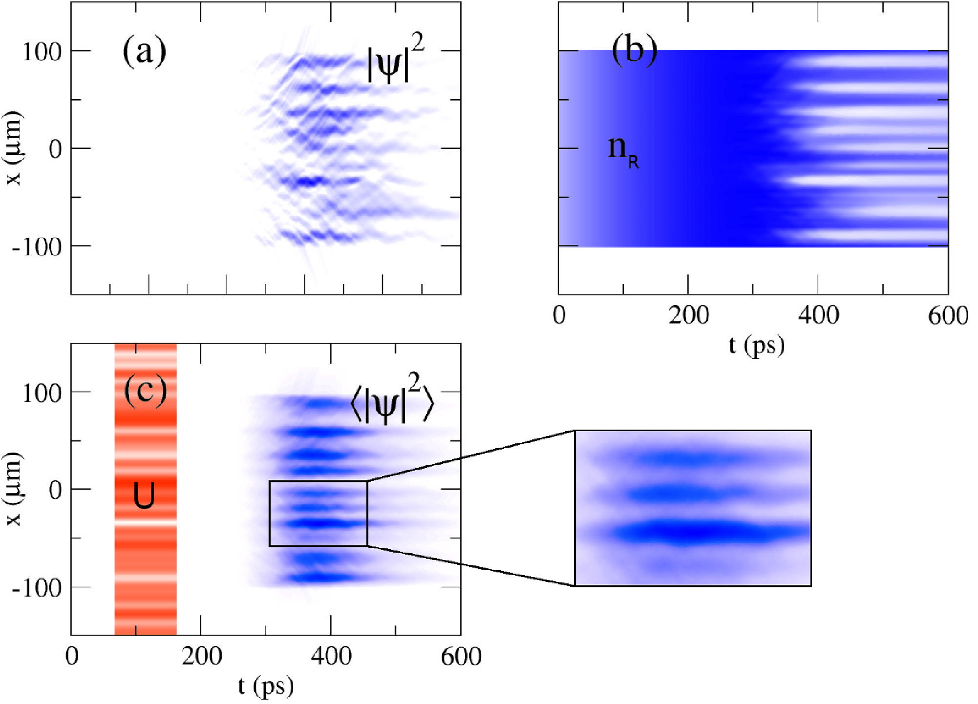
In Fig. 1 we present results of a typical simulation of the condensation process. The Figures 1(a) and (b) show the polariton and reservoir exciton density in a single simulation, which can be interpreted as a single experimental realization (pulse) [17]. The polariton condensate appears about ps after arrival of the pulse, in the form of areas of high density, complemented by areas of high reservoir exciton density. While the polariton domains appear to be vulnerable and erratic structures, exciton domains are much clearer due to the large exciton diffusion time. Here we included a realistic disorder potential with amplitude of a fraction of meV and correlation length of a few micrometers. We checked that the only visible effect of such disorder is to introduce preferential positions for the domains in the potential minima. The domain widths or other characteristics are not changed substantially if the disorder is removed from the model. Thus, the domain creation phenomenon is not directly caused by the potential, but related to symmetry breaking as in the Kibble-Żurek mechanism.
The polariton structures become much better defined when the density is averaged over many pulses, see Fig. 1(c). The disorder allows to pin the domains in certain regions of the sample, that would otherwise become smeared out over many pulses (see Appendix A). The apparent phase separation originates from the repulsion between polaritons and excitons. It is related to the existence of two stationary solutions to the homogeneous version of Eqs. (2). Substituting , and we get
| (5) | ||||||
where is the threshold value of the pumping intensity . Here we assumed that , which is a good approximation for the parameters used. The above (a) and (b) are the exciton and polariton phases, the latter existing only for .
The presence of the disorder adds another complication, as the polariton condensate has the tendency to be localized in its minima. We note that creation of domains through symmetry breaking and simple localization can, in principle, coexist in the same experiment – defect formation during the phase transition could be followed by localization in the potential minima at late stages of evolution. The question is whether the simple localization could mimic the defect formation, and how to distinguish between the two. We show that this can be easily achieved by investigating the dependence of the number of domains in function of the pumping intensity.
We consider a scenario (or a “control experiment”), where the pumping intensity is increased slowly. Such transition can be achieved eg. by using a continuous wave laser beam for pumping. This corresponds to a very slow phase transition, and a very large domain length scale in our model, larger than the system size L (we use switching time equal to 100ns which is long concerning the time scales of the system). In this case, polariton domains, or “condensates localized in the potential minima”, are still created, but their number is practically independent on the pumping intensity, see Fig. 2. The domains always appear in the potential minima, and there is no scaling law for the number of domains. This is in contrast with the case of excitation by a picosecond pulse, where the number of domains strongly depends on the peak intensity, see Fig. 3. We note that in this case the number of domains is never lower than the number of domains resulting from the localization in the potential minima.


IV Analysis of the domain formation process

Let us turn our attention to the early dynamics of the system. As shown on Fig. 4, after arrival of the pulse, first the free carrier density , and subsequently the reservoir exciton density increase gradually. The polariton field, on the other hand, is damped or amplified depending on the value of
| (6) |
The condition determines the critical point, and plays the role of the relative temperature [11]. We are not able to control directly, but through we can change the slope of at the critical point.
The crucial observation is that while remains small, the system is in a strongly nonequilibrium state, with the related timescale given by . There is practically no mixing of modes with different momenta, and the relaxation does not establish any relevant length scale. In other words, the weakness of interactions doesn’t allow for the effective thermalization that could lead to a quasi-equilibrium and the appearance of a condensed state. Contrary to the KZM picture, there is no well defined equilibrium before the phase transition, and the polariton mode occupation is shaped by the noise correlations (3). Moreover, as we show below, it is not these initial correlations that determine the final number of created defects.
The situation changes when the polariton-polariton interactions become sufficiently strong to compete with nonequilibrium processes, , with being a constant of the order of unity, and the average polariton density in the illuminated area. At this point , which can be identified as the condensation time [16], mode mixing starts to take place, which results in the appearance of an instantaneous quasi-equilibrium. The length scale associated with the emerging domains is established. The number of domains is determined by
| (7) |
In the following, we estimate the emerging length scale . We consider the dynamics of the system from the critical point crossed at up to the time when the condensate density reaches its maximum, , see Fig. 4. We are interested in the appearance of a length scale during the growth of the polariton field . At a very short time scale, much smaller than , , and , the total exciton density is a constant of motion of Eqs. (2). This allows to derive an effective equation, which in the case reads
| (8) |
where , , , and . We note that equation of the same form has been used by other authors to describe the polariton dynamics [18], with an important difference that the sign of the effective interaction is negative in the physically relevant case . Obviously, the above equation cannot model the long-time dynamics of repulsive particles, but is useful to describe dynamical instability on a short time scale.
Let us now assume that there exists a patch of approximately constant polariton field (a condensate seed), at . We can describe small fluctuations around by
| (9) |
where and are the chemical potential and the growth rate of the patch, and , represent the fluctuations. Substituting the above to (8) gives the Bogoliubov-de Gennes modes , and the mode frequencies
| (10) |
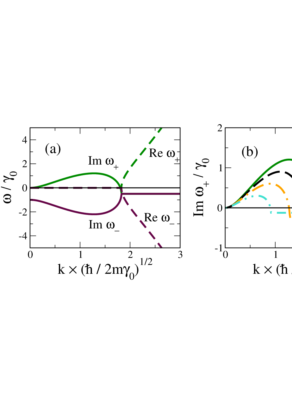
where , the saturation parameter , and for our parameters. As shown in Fig. 5, mode frequencies are complex in general, with unstable long-wave modes (Im ) below a certain value of . If the patch is larger than the length scale set by , dynamical instability will lead to the breakup or shrinkage of the patch. In the opposite case, the patch will expand due to damping of short-wavelength perturbations. This ”spectral filtering” is expected to produce structures with a well defined length scale . As shown in Fig. 5(b), this process is efficient for large values of the saturation parameter , when is comparable to . Such high polariton density is achieved when reaches its peak value, i.e. when , where is the maximum value of (see Fig. 4). This allows to estimate the length scale as .

In Figure 6 we plot the average number of created domains [19], according to numerical solutions of Eqs. (2) and (3). In the cases with the disorder , we average the result over 30 random disorder potentials of the same amplitude . For each of the disorder potentials, we run 50 simulations of the experiment with random Wigner noise and count the number of domains present on the average density profiles similar to Fig. 1(c). We also show the results of disorder-free cases, where the averaging is performed only over random Wigner noise realizations, and the number of domains is calculated using single-pulse pictures like Fig. 1(a),(b). We stress that in the latter case, domain counting could be preformed only in single-pulse measurements or through correlation measurements, since the average density profile contains no domains due to lack of pinning.
In the absence of disorder, the number of domains is clearly inversely proportional to over the pumping range of . The scaling prefactor appears to be exactly the same for two different values of and even for a qualitatively different temporal excitation. This provides a robust confirmation of our model. Figure 6(b) shows the predicted scaling of the approximate analytical model, see Appendix 10.

The presence of disorder has an important effect on the dynamics, as it is able “pin” the domains to certain positions in the sample, see Appendix A. This can be understood from the fact that the initial density fluctuations are suppressed in the areas of higher potential . Hence, it is more likely that condensate seeds will form in potential wells rather than hills. In the momentum space, this effect results in redistribution of mode occupation. In the lowest order approximation, this effect will be washed out in space by the consequent spectral filtering, leaving no fingerprint on the density of created domains. The fast exponential growth of selected modes would make any initial spectral mode occupation irrelevant. At the same time, domain positions in real space would essentially remain unaffected by the growth. Such approximation, however, doesn’t take into account the influence of the potential on the filtering process. In fact, in simulations with realistic disorder amplitude, we can see an increase of the number of domains with respect to the disorder-free case. This is especially visible for larger values of the disorder amplitude, as shown in Fig. 7. For the largest amplitude, meV, there is clearly a lower limit for the number of domains, which we identify with the the number of domains in the stationary state of the disorder potential, or the number of stationary condensates. This natural lower limit for may preclude the observation of scaling in samples with large amount of disorder. For the largest pumping intensity, the number of domains (light circles) may also deviate from the scaling law, which is associated with the instability of domains for strongest pumping and the associated difficulty in domain counting. This is also visible in large fluctuations of the domain number.
V Discussion
It is clear that some of the key elements of the KZM, such as the adiabatic-impulse-adiabatic scenario, or the “freezing” of correlation length before the phase transition, are not present in the condensation dynamics. Nevertheless, the scaling laws also result from the competition of timescales existing in the system. To obtain them, let us define “nonequilibrium” counterparts of critical exponents and with an analogue to the inverse correlation length, , and an analogue to the inverse relaxation time, . If we treat as an external control parameter that changes like , the local departure of the order parameter from the initial “vacuum” state is proportional to , and the quasi-equilibrium is achieved at , up to a logarithmic factor. The spectral cutoff at this point is , which gives the defect number . Remarkably, these formulas have identical forms as the standard KZM scalings (1). For example, in the present system we have and , which gives the correct prediction , see (16). Note that while the mechanism of spectral filtering is somewhat similar to phase ordering kinetics [20], contrary to the latter, it describes the stage of defect formation, and may be used to provide a starting point for the subsequent phase ordering.
VI Conclusions
In conclusion, we investigated the formation of coherence of exciton-polariton condensate in a one-dimensional nanowire. We demonstrated the spontaneous formation of exciton and polariton domains and found that the standard adiabatic-impulse-adiabatic scenario of the Kibble-Żurek theory cannot describe the system dynamics. Nevertheless, appropriately modified scaling laws are still present, which results from the competition between characteristic timescales in the system. Our study can have practical implications for applications proposed for polariton systems, as we point out the possible difficulty in creating a coherent condensate on a short timescale.
Acknowledgements.
We thank Jacek Dziarmaga for reading the manuscript and continuous stimulating discussions. This work was supported by the National Science Center grants DEC-2011/01/D/ST3/00482, DEC-2011/03/D/ST2/01938, and by the Foundation for Polish Science through the “Homing Plus” program.Appendix A Averaging over multiple pulses
While the disorder potential introduces some deviations from the scaling laws, its presence is useful for the observation of domains in a streak-camera experiment. In the absence of the disorder, the domains are created at random positions in the sample, and consequently the averaged luminescence intensity pattern becomes smeared out for a large number of pulses. Remarkably, the disorder potential with appropriate amplitude has the ability to “pin” the domains to certain preferred positions, which allows to obtain clear patterns even when averaging over very many pulses. The Figure 8 shows typical results of averaging. With the increase of the number of pulses the picture becomes clearer, while the intensity contrast is not diminished. The picture suggest that the picture will not change even after averaging over millions of pulses as in real experiments.

Appendix B Effect of the polariton energy relaxation
Several experiments [4, 21, 22] have shown that the polariton energy relaxation (or thermalization) may play an important role in their dynamics. To estimate the effect of relaxation due to the interactions with the exciton reservoir, which seems to be the dominant mechanism when the spatial overlap between the reservoir and the condensate is significant, we follow the phenomenological model of [4, 21, 22] by adding the additional term of the form to the right hand side of the polariton field equation. Here is the maximum density of exciton reservoir over the whole evolution, and the magnitude of the relaxation coefficient [21, 22] ranges from to . We find that for the effect of relaxation on the domain formation is negligible, and even for it does not affect the domain pattern structure, see Fig. 9. In the latter case, the domain pattern is smoothed out, which is due to the additional damping of short-wave fluctuations.

Appendix C Defect formation vs. the hole-burning effect
Our model predicts the creation of defects due to the special form of the Bogoliubov excitation spectrum during the buildup of the polariton phase. It was demonstrated [3] that the excitation spectrum of a steady-state polariton condensate can also develop a similar band of unstable modes at at small , which may give rise to a ’hole-burning’ effect, and formation of polariton and reservoir exciton domains. However, we found that this effect alone cannot explain our results. In particular, domains are formed also when the steady-state excitation spectrum does not exhibit any instability, as shown in Fig. 10. Consequently, the phenomenon we describe is a dynamical effect, and cannot be explained by the analysis of a steady-state solution.

Appendix D Analytical model of system dynamics
When introducing our model we suggest that the number of domains is controlled by the rate at which the critical point is crossed, in analogy to the theory of the Kibble-Żurek mechanism. As shown in Fig. 2 in the main text, the reservoir exciton density grows approximately linearly at the critical point , which allows to make analytical predictions about the resulting length scale . To this end, we neglect the loss terms to obtain, in the case of a Gaussian excitation pulse , an analytical solution for and in the illuminated area
| (11) | ||||
| (12) |
where . Initially, the polariton density grows roughly like
| (13) |
where is the initial polariton occupation determined by the Wigner noise and is the time when the critical point is crossed. Density saturates at , at the time approximately equal to
| (14) |
Note that up to a logarithmic factor. We can now estimate
| (15) |
Since as discussed in the text, we obtain the approximate scaling law
| (16) |
When looking at evolutions at different pumping intensities, we encounter universal behavior due to the scaling laws for the Bogoliubov frequencies. Since we may write , where gives the time scale of the growth, and up to a logarithmic factor, we have
| (17) |
References
- [1] J. Kasprzak et al., Nature (London) 443, 409 (2006).
- [2] S. Christopoulos et al., Phys. Rev. Lett. 98, 126405 (2007); A. Amo, J. Lefrère, S. Pigeon, C. Adrados, C. Ciuti, I. Carusotto, R. Houdré, E. Giacobino, and A. Bramati, Nat. Phys. 5, 805 (2009); G. Nardin, G. Grosso, Y. Léger, B. Piȩtka, F. Morier-Genoud, and B. Deveaud-Plédran, Nat. Phys. 7, 635 (2011); K. G. Lagoudakis, B. Pietka, M. Wouters, R. André, and B. Deveaud-Plédran, Phys. Rev. Lett. 105, 120403 (2010); P. Stȩpnicki, and M. Matuszewski, Phys. Rev. A 88, 033626 (2013); H. Deng, H. Haug, and Y. Yamamoto, Rev. Mod. Phys. 82, 1489 (2010). I. Carusotto and C. Ciuti, Rev. Mod. Phys. 85, 299 (2013).
- [3] M. Wouters and I. Carusotto, Phys. Rev. Lett. 99, 140402 (2007).
- [4] E. Wertz et al., Nat. Phys. 6, 860 (2010).
- [5] K. G. Lagoudakis, F. Manni, B. Pietka, M. Wouters, T. C. H. Liew, V. Savona, A. V. Kavokin, R. André, and B. Deveaud-Plédran, Phys. Rev. Lett. 106, 115301 (2011).
- [6] T. C. H. Liew, A. V. Kavokin, and I. A. Shelykh, Phys. Rev. Lett. 101, 016402 (2008); I. A. Shelykh, A. V. Kavokin, Y. G. Rubo, T. C. H. Liew, and G. Malpuech, Semicond. Sci. Technol. 25, 013001 (2010); C. Adrados, T. C. H. Liew, A. Amo, M. D. Martín, D. Sanvitto, C. Antón, E. Giacobino, A. Kavokin, A. Bramati, and L. Viña, Phys. Rev. Lett. 107, 146402 (2011); D. Ballarini et al., arXiv:1201.4071 (2012).
- [7] A. V. Kavokin, I. A. Shelykh, T. Taylor, and M. M. Glazov, Phys. Rev. Lett. 108, 197401 (2012).
- [8] B. Damski and W. H. Żurek, Phys. Rev. Lett. 104, 160404 (2010).
- [9] G. Nicolis and I. Prigogine, Self-organization in nonequilibrium systems: from dissipative structures to order through fluctuations (Wiley, 1977); H. Haken, Synergetics: An Introduction : Nonequilibrium Phase Transitions and Self-Organization in Physics, Chemistry and Biology (Springer, Berlin, 1978); G. Ódor, Rev. Mod. Phys. 76, 663 (2004); H. Hinrichsen, Physica A 369, 1 (2006).
- [10] T. W. B. Kibble, J. Phys. A 9, 1387 (1976); T. W. B. Kibble, Phys. Rep. 67, 183 (1980).
- [11] W. H. Żurek, Nature (London) 317, 505 (1985); W. H. Żurek, Phys. Rep. 276, 177 (1996); C. Bauerle et al., Nature (London) 382, 332 (1996); V.M.H. Ruutu et al., ibid. 382, 334 (1996).
- [12] I. Chuang et al., Science 251, 1336 (1991); A. Maniv, E. Polturak, and G. Koren, Phys. Rev. Lett. 91, 197001 (2003); L. E. Sadler, J. M. Higbie, S. R. Leslie, M. Vengalattore, and D. M. Stamper-Kurn, Nature (London) 443, 312 (2006); C. N. Weiler et al., Nature (London) 455, 948 (2008); E. Witkowska, P. Deuar, M. Gajda, and K. Rza̧żewski, Phys. Rev. Lett. 106, 135301 (2011); J. Dziarmaga, Phys. Rev. Lett. 95, 245701 (2005);
- [13] A. Janot, T. Hyart, P. R. Eastham, and B. Rosenow, Phys. Rev. Lett. 111, 230403 (2013); L. M. Sieberer, S. D. Huber, E. Altman, and S. Diehl, Phys. Rev. Lett. 110, 195301 (2013).
- [14] I. Carusotto and C. Ciuti, Phys. Rev. B 72, 125335 (2005); M. Wouters and V. Savona, Phys. Rev. B 79, 165302 (2009); D. Read, T. C. H. Liew, Y. G. Rubo, and A. V. Kavokin, Phys. Rev. B 80, 195309 (2009); A. Chiocchetta and I. Carusotto, Europhys. Lett. 102, 67007 (2013).
- [15] J. Szczytko, L. Kappei, J. Berney, F. Morier-Genoud, M. T. Portella-Oberli, and B. Deveaud, Phys. Rev. Lett. 93, 137401 (2004); F. Veit, M. Aßmann, M. Bayer, A. Löffler, S. Höfling, M. Kamp, and A. Forchel, Phys. Rev. B 86, 195313 (2012).
- [16] A. V. Kavokin, J. J. Baumberg, G. Malpuech, and F. P. Laussy, Microcavities (Oxford University Press, Oxford, 2007).
- [17] A. Sinatra, C. Lobo, and Y. Castin, J. Phys. B 35, 3599 (2002); A. Polkovnikov, Ann. Phys. 325, 1790 (2010).
- [18] J. Keeling and N. G. Berloff, Phys. Rev. Lett. 100, 250401 (2008); M. Wouters and I. Carusotto, Phys. Rev. Lett. 105, 020602 (2010); J. Cuevas, A. S. Rodrigues, R. Carretero-González, P. G. Kevrekidis, and D. J. Frantzeskakis, Phys. Rev. B 83, 245140 (2011).
- [19] To determine the number of domains we count the number of zero crossings of the function , where is the maximum of local polariton density over the entire experiment, at the time instant when the number of these crossings is the largest. We checked that this method gives reliable estimation of . In the disorder-free case, we count domains in single-pulse experiments using the exciton density profile instead of the polariton density .
- [20] A.J. Bray, Adv. Phys. 43, 357 (1994).
- [21] E. Wertz, A. Amo, D. D. Solnyshkov, L. Ferrier, T. C. H. Liew, D. Sanvitto, P. Senellart, I. Sagnes, A. Lemaître, A. V. Kavokin, G. Malpuech, and J. Bloch, Phys. Rev. Lett. 109, 216404 (2012).
- [22] D. Tanese, H. Flayac, D. Solnyshkov, A. Amo, A. Lemaître, E. Galopin, R. Braive, P. Senellart, I. Sagnes, G. Malpuech, and J. Bloch, Nature Commun. 4, 1749 (2013).