Correlations in non-equilibrium Luttinger liquid and singular Fredholm determinants
Abstract
We study interaction-induced correlations in Luttinger liquid with multiple Fermi edges. Many-particle correlation functions are expressed in terms of Fredholm determinants , where and have multiple discontinuities in energy and time spaces. Such determinants are a generalization of Toeplitz determinants with Fisher-Hartwig singularities. We propose a general asymptotic formula for this class of determinants and provide analytical and numerical support to this conjecture. This allows us to establish non-equilibrium power-law singularities of many-particle correlation functions. As an example, we calculate a two-particle distribution function characterizing correlations between left- and right-moving fermions that have left the interaction region.
pacs
73.23.-b, 73.50-TdNon-equilibrium phenomena in (effectively) one-dimensional correlated systems—including Kondo and related quantum impurity models [1, 2, 3, 4, 5, 6, 7], quantum Hall edge interferometry [8, 9, 10, 11, 12] and energy relaxation [13, 14], carbon nanotube tunneling spectroscopy [15], Fermi edge singularity [16], and correlated electrons in quantum wires [17, 18, 19, 20, 21, 22, 23]—are attracting lots of experimental and theoretical interest. In these problems applied voltages lead to formation of distribution functions with two or more Fermi edges, which generates non-equilibrium scaling, criticality and decoherence. A remarkable property of the Luttinger liquid (LL) model is a possibility of exact solution even for such non-equilibrium distributions. In this paper we show how many-particle fermionic correlation functions can be calculated and discuss the underlying physics. It turns out that are given by a certain type of singular Fredholm determinants. Our result for the asymptotics of such determinants is expected to be relevant also to other non-equilibrium many-body problems.
In previous works [19, 20, 21], we have shown that single-particle Green function (GF) in the case of LL (and in a number of related problems) can be expressed through Fredholm determinants of a “counting” operator
| (1) |
where operators and are diagonal in the time and energy representations, respectively, and . The one-particle distribution function characterizes the non-equilibrium state of incoming electrons, while the time-dependent phase encodes the information about the interaction. For a LL adiabaticaly connected to reservoirs the phase is [19]
| (2) |
where is the Heaviside step function. This allows one to reduce the operator in Eq. (1) to a Toeplitz matrix [21], with determining its symbol. (For a non-adiabatic coupling one gets a sequence of rectangular pulses in , yielding in the long-wire limit a product of Toeplitz determinants.) When has discontinuities (“Fermi edges”), the single particle GF acquires a non-trivial power-law behavior. This is in particular the case for multi-step distributions
| (3) |
The low-energy behavior of the single-particle correlation functions can be understood with the help of the generalized version [21, 23] of the Fisher-Hartwig conjecture [24] (see also [25, 26]). Under generic conditions, it yields a power-law energy dependence masked by dephasing [21, 23]. When the electronic system is in a pure state, i.e. for (3) with all equal or , the dephasing is absent and the effects of correlations are particularly strongly pronounced.
Higher-order GF of a non-equilibrium LL can be cast in the form Eq.(1) as well, which offers a remarkable opportunity of exploring many-particle correlations in a quantum many-body system out of equilibrium. However, there is a serious complication as compared to the single-particle GF case. Since each creation or annihilation of an electron induces a jump in , the latter has a form
| (4) |
As we see, the determinant is now generated by functions and that both have multiple jumps and therefore is not of Toeplitz type. Since time and energy enter Eq. (1) on equal footing, one may expect the and discontinuities to play a similar role in the asymptotic behaviour. This suggests that there should exist a generalization of the Fisher-Hartwig formula valid for this class of determinants. This generalization represents one of key results of the present paper.

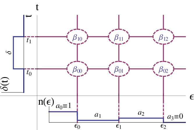
We first state our result for the long-time behavior of the determinant (1) and then present arguments in favor of it. To formulate the result, it is convenient to draw a grid in the time-energy plane defined by points where and exhibit jumps, as shown in Fig. 1 (for the case ). This divides the plane in rectangles (with the “external” ones extending to infinity). With each of them we associate a number
| (5) |
We impose the condition that a branch of the logarithm at infinity is fixed by and , while for finite pieces any branch can be chosen. We now define a matrix
| (6) |
where indices and correspond to the grid lines [27], and a set of exponents
| (7) |
The asymptotic behaviour of the normalized (to its zero-temperature form) determinant is given by
| (8) | |||||
Here the sum runs over all possible branches of the logarithms in (5), and are numerical coefficients [28]. Equation (8) represents the infrared asymptotics which holds provided that for all and . If for some set the opposite inequality holds, the corresponding factor should be dropped in (8). When all inequalities are fulfilled, one can calculate the total power of each of the factors and in (8) by using the sum rules and , which yields
| (9) | |||||
where , , and is the ultraviolet cutoff.
While we have no mathematical proof of Eq. (8), we have strong evidence in favor of its validity. Heuristically, Eq. (8) represents a natural extension of the generalized Fisher-Hartwig formula of Refs. [21, 23] (valid for Toeplitz determinants) onto the present case. Indeed, the Fisher-Hartwig formula suggests that power-law factors in the asymptotics of Toeplitz determinants are due to the presence of singular points and each pair of such points contributes independently to the result. Physically, the contribution of the pair of points and represents the effect of particle-hole pair scattering from the vicinity of the Fermi edge to Fermi edge within the time . Combined with the symmetry between and , these arguments naturally lead to Eq. (8). On a technical level, we have proven a generalization of strong Szegő limit theorem [29, 30] to the case of a multistep and smooth . Substituting in this formula a multi-step , we obtain logarithmic divergencies in the exponent, yielding power laws of Eq. (8). We refer the reader to Supplementary Material [32] for detail. Finally, we evaluated the determinant numerically for the simplest non-Toeplitz case, with having three jumps. The results [32] confirm Eq. (8).


We now apply Eq.(8) to the problem of correlations in a non-equilibrium LL. We consider a LL conductor of length (characterized by LL parameter ) driven out of equilibrium via the injection of electrons with distributions [ () for right- (left-) movers] from the non-interacting leads, see Fig. 1 of Ref.[31]. To be specific, we assume that the right-moving electrons have the triple-step distribution function with population inversion (Fig. 2) while the left movers are at zero temperature. This is the simplest non-equilibrium setup without dephasing. The width of is set to unity, thus determining the time and energy scale of the problem. We model the leads by 1D conductors with . The correlations effects discussed in this paper can be traced back to the scattering of LL plasmons at the boundaries of the wire. This scattering is strong when boudaries are sharp (compared to the plasmon wave length), , so that we focus on this regime. We stress that we assume the absence of the electron backscattering in the wire, i.e., is smooth on the scale of the Fermi wavelength.
At thermal equilibrium ( are Fermi-Dirac distributions with equal temperatures), the interaction causes no correlations for electrons outside the LL wire. In other words, electrons leave the wire in the same state as free fermions would do at given temeparture. The situation changes dramatically under non-equilibrium conditions [31]. The plasmon scattering at the boundaries of the wire (characterized by reflection coefficient and transmission coefficient ) not only leads to an electron energy redistribution but also induces correlations between outgoing electrons. As we found earlier [31], distribution functions in the non-interacting regions are given (up to a numerical factor) by the determinant (1) with phases and shown in Fig. 3. Both phases consist of an infinite sequence of rectangular pulses separated by a time interval . In the long-wire limit the corresponding determinant can be decomposed into the product of Toeplitz determinants controlled by individual pulses [33]. An asymptotic analysis of these determinants [23] leads to the conclusion that distribution functions of outgoing electrons have power-law singularities at the Fermi edges (Fig. 2). Note that for relatively weak interaction the interaction effects are most pronounced at the inverted edge of the signaling that the dominant physical process is the scattering of electron-hole pairs from this edge to the Fermi edge of .
To reveal the correlations induced by the plasmon scattering, we consider the irreducible two-particle distribution function of outgoing electrons in the two leads, with and . It is a non-trivial function of , with the correlations being most pronounced in a vicinity of the points [31]. We focus on the case where the correlations are maximal. At this point the function is given by the determinant (1) with the phase , see Fig. 3. Explicitly
| (10) | |||||
Investigation of the correlations of left- and right- movers is now reduced to calculation of the Fredholm determinant with phase that can be readily done by employing Eq. (8). For a long wire the determinant decomposes into a product of determinants corresponding to individual pulses forming (see Fig. 3). We write , where is a contribution of the first pulse and of the remaining pulses. For definiteness, we focus on the case of a weak interaction (small ) when the phase is small outside the first pulse. Accordingly, the asymptotic behavior of the determinants for all pulses but the first one is governed by a single term in the sum (8) corresponding to a choice of logarithm branches such that for all and . [The analysis for an arbitrary interaction proceeds in the same way; one just may need to take into account several further terms in Eq. (8).] This yields
| (11) |
To find , we note that is close to ; an inspection of Eq. (8) leads to the following three dominant contributions:
| (12) | |||||
Since we are not interested in the dependence on energies , we have absorbed it in the coefficients in Eqs. (11) and (12). Combining (11) and (12) with asymptotic expansion for the Toeplitz determinants and [32], we arrive at the asymptotic expansion of irreducible correlation function in time domain.
The two-particle correlation function is shown in Fig. 4 for . The left panel presents the results of direct numerical evaluation of the Fredholm determinants, while the middle panel displays the asymptotics given by Eqs. (11) and (12) with the coefficients used as fitting parameters. As expected, the asymptotics based on Eq. (8) reproduces correctly the behavior of outside the region of -plane where or , or .
Power-law long-time behavior translates into singularities in the energy reperentation of the correlation function plotted in right panel of Fig.4. Strong correlations are observed that form a “crest” going along the line (thick red line). The analysis shows that the main contribution to this structure in comes from the vicinity of the main diagonal of the -plane. In this region, the main contribution to Eq. (12) is given by the last term yielding with , whereas Eq. (11) reduces to with . This yields the behavior of near the crest
| (13) |
Physically, the crest originates from intensive scattering of electron-hole pairs from the vicinity of the left-mover Fermi surface to the inverted Fermi surface of right movers, and Eq. (13) can be viewed as a Fermi-edge singularity in a higher-order correlation function.
To summarize, we have studied correlation induced by interaction in a non-equilibrium LL. We have shown that electron scattering between multiple Fermi edges leads to power-law singularities in many-particle distribution functions. As a particular example, we calculated a two-particle distribution function characterizing correlations between left- and right-moving outgoing fermions. Technically, many-particle correlation functions are expressed in terms of Fredholm determinants , where and have multiple discontinuities in energy and time spaces, respectively. We have conjectured a general asymptotic formula for this class of determinants and provided an ample analytical and numerical support to this conjecture. The results are expected to be relevant to a broad class of non-equilibrium many-body problems including the Kondo problem; work in this direction is currently underway.
We acknowledge support by Alexander von Humboldt Foundation, ISF, and GIF.
Appendix A Analytical justification of the asymptotic formula for singular Fredholm determinants
In this section we present analytical arguments in favor of the Eqs. (8), (9) of the main text for the asymptotic behavior of the determinants with and having multiple discontinuities in energy and time spaces, respectively. We begin [Sec. A.1] by reminding the reader about Szegő formula for Toeplitz matrices with smooth symbols and a generalized version of the Fisher-Hartwig formula for Toeplitz matrices with singular symbols. We emphasize there a connection between these two formulas. We proceed then by formulating and presenting a proof of a generalization of Szegő formula for the case of a multi-step function and smooth , Sec. A.2. Finally, in Sec. A.3 we use this result to obtain the scaling behavior of Fredholm determinants in the case when both functions and have multiple singularitites.
A.1 Toepliz determinants: Strong Szegő limit theorem and generalized Fisher-Hartwig conjecture
Let us consider the determinant of Toeplitz matrix , generated by function defined on the unit circle and having sufficiently smooth logarithm . We use the notation
| (14) |
Smoothness of on the unit circle implies the existence of the Wiener-Hopf decomposition for
| (15) |
with functions being analytic inside and outside the unit circle respectively. In terms of Fourier components of
| (16) |
The strong Szegő limit theorem [29] states that under the assumptions made above the asymptotic behavior of the Toeplitz determinant at is given by
| (17) |
When interpreted in physical terms Eq.(17) yields the long-time asymptotic of the single-particle correlation functions of interacting fermions in a non-equilibrium state characterized by smooth distribution function [21]. The exponential term in (17) encodes herewith the information about the oscillations of the Green functions and its exponential decay due to non-equilibrium dephasing, while the precise value of the pre-exponential factor is of little importance.
The situation changes significantly if one considers single-particle Green functions in a state characterized by distribution function of electrons having discontinuities (Fermi edges). To be specific we limit our discussion to the case of multi-step distribution function
| (18) |
Supplementing the theory with the ultraviolet cutoff , one ends up with a Toeplitz matrix with symbol having jumps. In the context of Toeplitz matrices such discontinuitites are known as Fisher-Hartwig singularities. More specifically, the symbol of interest is
| (19) | |||
| (20) |
with and
| (21) |
Here the numbers controlling the jumps of at points are given by
| (22) |
We are interested in the large- asymptotic behavior of the determinant . In physical language the size of the Toeplitz matrix corresponds to the time in the correlation function .
Strictly speaking, the strong Szegő theorem does not apply to the Toeplitz matrix with a singular symbol (19); the corresponding extension of the large- limit theorem is known as Fisher-Hartwig conjecture [34]. This conjecture states that at large
| (23) |
with being a (known) numerical coefficient. Casting this result in terms of physical variables and assuming that all energies are small compared to , one obtains
| (24) |
While a rigorous mathematical proof of Eq.(24) is highly non-trivial and for the general settings was achieved only very recently, a strong argument in favor of Eq.(24) can be given on the basis of the Szegő formula (17). Indeed, the jumps of at points dictate the following asymptotic behavior of the Fourier coefficients at
| (25) |
The naive application of the Szegő formula leads now to
| (26) |
where we have introduced here .
Equation (26) can be given a pictorial representation shown in Fig.5. We attribute the quantities to the points in -plane where jumps of the functions and cross. Each pair of such points with different time arguments [i.e., and for )] provides the following contribution to the last factor in Eq. (26):
| (27) |
To give meaning to this expression, we have to cut off the logarithmically diverging integral. The lower integration limit is set naturally by the ultraviolet cutoff . For one expect the upper integration limit to be given by the time . On the other hand, for the upper limit of integration is expected to be (recall that the asymptotics we are discussing is valid under condition ). Using these simple cutoff rules together with the expression (20) for the coefficient , we see that the Szegő theorem justifies in a natural way the Fisher-Hartwig conjecture (24).
There is, however, the following subtlety here. Recalling the definition (19) of the symbol with Fisher-Hartwig singularities, one sees that the numbers are defined modulo a set of integer numbers such that
| (28) |
In other words two sets of coefficients and describe the same symbol and should produce the same asymptotics. The recently proven rigorous formulation of the Fisher-Hartwig conjecture [24] indeed respects this requirement. Specifically, it states that one should choose the set of in Eq. (24) in such a way that the sum determining the power of takes the smallest possible value.
More recently, it was shown in [21, 23] that other choices of integer shifts (i.e. of logarithm branches) in the expressions for are also important and determine the sub-leading terms in the asymptotic behavior of a Toeplitz determinant with a singular symbol. A generalized Fisher-Hartwig conjecture formulated in this work reads
| (29) |
The summation here goes over all choices of , i.e., over all sets of integer shifts satisfying Eq. (28). Each such set yields in Eq. (29) a term with a distinct oscillatory exponent . Equation (29) presents explicitly the leading asymptotic behavior for the factor multiplying each of these exponents. Apart from this dominant term, there will be in general also subleading (in powers of ) terms corresponding to the same exponent; these are abbreviated by in the last bracket.
While a rigorous proof of the generalized Fisher-Hartwig conjecture Eq. (29) remains to be constructed, there is little doubt that it is correct.
A.2 Multiple singularities in : Generalization of Szegő formula
We assume now that the electronic distribution is a smooth function of energy, whereas the scattering phases has a multi-step structure:
| (30) |
We will assume for definiteness that ; generalization to a larger number of steps in is completely straightforward. Among known derivations of Szegő formula, the operator-theory approach due to Widom [30] permits a particularly transparent generalization to our problem. We thus follow this approach here.
Upon introduction of an ultraviolet cutoff the functional determinant of interest
| (31) |
is reduced to the determinant of a finite matrix of the size with the structure
| (32) |
Here stands for a rectangular Toeplitz matrix of the size with a symbol
| (33) |
which is smooth on the unit circle . The numbers and are determined by via
| (34) |
Let us introduce a semi-infinite Hankel matrix with symbol according to
| (35) |
and the semi-infinite matrices and with matrix elements ()
With this notations matrix can be presented in the form
| (41) |
Here the symbol is obtained from a symbol according to
| (42) |
The block representation (41) of the matrix allows us to write its determinant in the form
| (43) |
We have used here that . It is important that the last determinant in Eq. 43 has a finite limit as and go to infinity,
| (44) |
Here stands for semi-infinite Toeplitz matrix with symbol . We can now use simple properties of semi-infinite Toeplitz and Hankel matrices [30]
| (45) | |||
| (46) |
to bring the expression for constant to the form
| (47) |
On the other hand, one can recast the Szegő result (17) into the form[30]
| (48) |
Combining now Eqs. (47) and (48) we get for the determinant of interest
| (49) |
where is the zero Fourier component of . The derivation above can be immediately generalized to the case of having arbitrary number of steps, Eq.(30). The resulting determinant reads
| (50) |
with
| (51) | |||
| (52) |
Note that by definition
| (53) |
Equation (50) allows to reduce the problem of asymptotic behavior of to the evaluation of a determinant of a product of semi-infinite Toeplitz matrices. This is a crucial step forward because it enables us to apply the Winer-Hopf method to the problem. Specifically, let us introduce the Wiener-Hopf decomposition of the functions ,
| (54) |
Here are analytic inside (outside) the unit circle. The analytic properties of allow us to write
| (55) |
Thus
| (56) |
Note that due to the relation (53)
| (57) |
and one could naively conclude that the determinant in (56) is equal to unity. This is not true, however, due to the infinite size of the matrices involved. Instead, one should make use of the formula [35]
| (58) |
valid for arbitrary set of operators satisfying . Here stands for the commutator. Applying (58) to (56), we obtain
| (59) |
Finally, evaluating the traces one finds
| (60) |
Equation (60) is the generalization of the Szegő limit theorem to the case of determinants with a multi-step [and smooth ] and constitutes the main result of this subsection. In the next subsection we will analyze its implications for the case when is not smooth but rather has multiple steps.
A.3 Multiple singularities in and in : Further generalization of Fisher-Hartwig conjecture
We consider now the case when not only the phase but also the distribution function has multiple step-like singularities, Eq. (18). We will apply the generalized Szegő formula Eq. (60) derived above to this situation and then cut off the resulting logarithmic divergencies. While this is not a mathematically rigorous procedure, we should get in this way correct results for power-law exponents (apart from the summation over branches of the logarithms), cf. Sec. A.1.
The relevant functions are now given by
| (61) |
with
| (62) |
and
| (63) |
Here we have intriduced the notation
| (64) |
The coefficients can be assigned to the singular points in plane, as illustrated in Fig. 6.
Just as in Sec. A.1 coefficients control the asymptotic behavior of at ,
| (65) |
Applying now Eq. (60) with the cutoff procedure discussed in Sec.A.1 and representing the result in terms of physical variables, we find an asymptotic behavior of the determinant of interest
| (66) |
where we have used the condition
| (67) |
In full analogy with the case of Toeplitz determinants with Fisher-Hartwig singularities, see Sec. A.1, Equation (66) suffers from the ambiguity in the choice of . Pursuing this analogy, we conclude that the correct generalization of (66) involves a summation over all possible choices of ,
| (68) |
The summation over here can be understood as summation over all possible branches of logarithms in the definition of , Eq. (64), with the additional constraints imposed [cf. Eq.(28)]
| (69) |
A particular case of (68) is the zero temperature determinant
| (70) |
with . This result can also be checked by a direct calculation using the fact that at equilibrium the determinant is a gaussian functional of .
Equation (68) can be represented in a more symmetric way. Employng the condition
| (71) |
(valid for arbitrary multi-step distribution) and combining it with (68) and (70) we arrive at the (cutoff independent) asymptotic of the normalized determinant ,
| (72) |
where we have introduced the exponents
| (73) |
Let us now discuss the applicability of the long time asymptotic expansion. Throughout the derivations of Eq. (72), it was assumed that the area of all the rectangles in the time-energy plane is large, i.e., for any , , and
| (74) |
A straightforward extension of the cutoff procedure shows that asymptotics (72) remains valid even if for some sets the condition (74) is not satisfied, provided one drops the corresponding factors from the product (72).
Appendix B Factorization of the determinant for consisting of several remote pulses
In this section we discuss the determinant for the phase consisting of several rectangular pulses separated by large time intervals. We show that in this limit the determinant is given by a product of Toeplitz determinants corresponding to individual rectangular pulse. This question is relevant for the calculation of correlation functions in Luttinger liquid within generic boundaries (and in particular for “sharp boundary” model). In our current analysis we rely on Eq.(68).
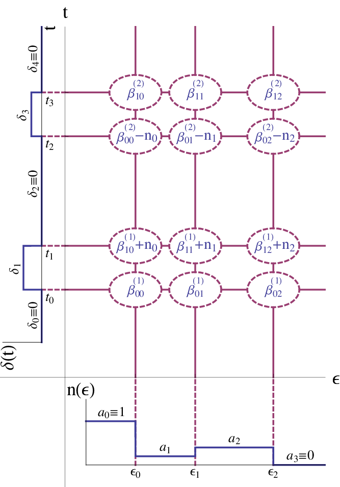
Let us consider counting field given by (see Fig. 7)
| (75) |
Our aim is to show that as goes to infinity, decouples into the product , with and being the two rectangular pulses constituting .
Let us introduce coefficients with corresponding to the phases and . Figure 7 demonstrates the connection between the coefficients corresponding to and . Here we have introduced a set of integers satisfying . Let us consider a particular term in the sum (68) corresponding to the given set of coefficients and set of integers . The dependence of this term on at is easily found to be
| (76) |
We see that only terms of the sum (68) characterized by , for survive the limit . Thus we find that in the long-time limit the determinant in question factorizes into a product of Toeplitz determinants
| (77) |
This factorization was proposed in Ref.[20, 19] on the basis of physical arguments and employed to calculate single-particle Green functions. In the main text of the present paper we also use an analogous factorization for the case of two-particle correlation functions.
Appendix C Numerical check for the asymptotics (72) of determinants with multiple and discontinuities


In this section we present a numerical verification of the asymptotic formula (72) for determinants with multiple discontinuities both in and in . We calculate numerically the normalized Fredholm determinant with a triple-step counting field (see inset of Fig.8)
| (78) |
as a function of and and compare results to the predictions of Eq.(72). The energy distribution is taken to be
| (79) |
with , and . The numerical procedure used here is based on the time discretization and is analogous to the one employed in Ref. [23] in course of studies of Toeplitz determinants.
Taking into account that and in (78) are close to , one infers the following three dominant contributions to the sum (72):
| (80) |
Here we have absorbed the dependence of the determinant on energies into the coefficients .
The exponents in (80) are given by
| (81) | |||
| (82) | |||
| (83) | |||
| (84) | |||
| (85) | |||
| (86) |
A characteristic feature of the exponents (81)—(86) is their smallness at .
The upper panel of Fig.8 shows the real part of the determinant . The solid blue lines on both graphs represent the results of numerical evaluation of Fredholm determinant. Each curve corresponds to the fixed time ( for curves mark by letters from “a” to “e”, respectively) while changes from to . Dashed lines show the fit of numerical result by expression (80) with coefficients , and considered as fitting parameters. The same set of is used for all curves. We see that the fit reproduces correctly the overall behavior of the determinant but the oscillations with time are not captured in this approximation. An analysis of (72) shows that for chosen parameters the dominant correction to (80) is given by
| (87) |
with
| (88) | |||
| (89) | |||
| (90) |
Taking the correction (87) into account, we obtain a fit to numerical data (bottom panel of Fig. 8) which correctly captures the oscillation in time. The resulting agreement is essentially perfect. We thus conclude that our conjecture, Eq. (72), is fully supported by the numerical simulations.
References
- [1] D. Goldhaber-Gordon, H. Shtrikman, D. Mahalu, D. Abusch-Magder, U. Meirav, and M. A. Kastner, Nature 391, 156 (1998); R. M. Potok, I. G. Rau, H. Shtrikman, Y. Oreg, and D. G. Goldhaber-Gordon, ibid. 446, 167 (2007).
- [2] A. Rosch, J. Kroha, and P. Wölfle, Phys. Rev. Lett. 87, 156802 (2001); A. Rosch, J. Paaske, J. Kroha, and P. Wölfle, ibid. 90, 076804 (2003); J. Paaske, A. Rosch, and P. Wölfle, Phys. Rev. B 69, 155330 (2004); J. Paaske, A. Rosch, J. Kroha, and P. Wölfle, ibid. 70, 155301 (2004); S. Kehrein, Phys. Rev. Lett. 95, 056602 (2005); L. Borda, K. Vladar, and A. Zawadowski, Phys. Rev. B 75, 125107 (2007); R. Gezzi, Th. Pruschke, and V. Meden, ibid. 75, 045324 (2007); C.-H. Chung, K.V.P. Latha, K. Le Hur, M. Vojta, P. Woelfle; ibid. 82, 115325 (2010); A. Mitra and A. Rosch, Phys. Rev. Lett. 106, 106402 (2011).
- [3] S. De Franceschi, R. Hanson, W. G. van der Wiel, J. M. Elzerman, J. J. Wijpkema, T. Fujisawa, S. Tarucha, and L. P. Kouwenhoven, Phys. Rev. Lett. 89, 156801 (2002).
- [4] R. Leturcq, L. Schmid, K. Ensslin, Y. Meir, D.C. Driscoll, and A.C. Gossard, Phys. Rev. Lett. 95, 126603 (2005).
- [5] J. Paaske, A. Rosch, P. Wölfle, N. Mason, C. M. Marcus, and J. Nygard, Nat. Phys. 2, 460 (2006).
- [6] A. Mitra and A.J. Millis, Phys. Rev. B 76, 085342 (2007).
- [7] S. T. Carr, D. A. Bagrets, and P. Schmitteckert, Phys. Rev. Lett. 107, 206801 (2011).
- [8] Y. Ji, Y.C. Chung, D. Sprinzak, M. Heiblum, D. Mahalu, and H. Shtrikman, Nature 422, 415 (2003); I. Neder, M. Heiblum, Y. Levinson, D. Mahalu, and V. Umansky, Phys. Rev. Lett. 96, 016804 (2006); I. Neder, M. Heiblum, D. Mahalu, and V. Umansky, ibid. 98, 036803 (2007); I. Neder, F. Marquardt, M. Heiblum, D. Mahalu, and V. Umansky, Nature Phys. 3, 534 (2007).
- [9] P. Roulleau, F. Portier, D.C. Glattli, P. Roche, A. Cavanna, G. Faini, U. Gennser, and D. Mailly, Phys. Rev. B 76, 161309 (R) (2007); P. Roulleau, F. Portier, P. Roche, A. Cavanna, G. Faini, U. Gennnser, and D. Mailly, Phys. Rev. Lett. 100, 126802 (2008); ibid. 101, 186803 (2008); ibid 102, 236802 (2009); P-A. Huynh, F. Portier, H. le Sueur, G. Faini, U. Gennser, D. Mailly, F. Pierre, W. Wegscheider, P. Roche, ibid. 108, 256802 (2012).
- [10] L.V. Litvin, H. P. Tranitz, W. Wegscheider, and C. Strunk, Phys. Rev. B 75, 03315 (2007); L.V. Litvin, A. Helzel, H. P. Tranitz, W. Wegscheider, and C. Strunk, ibid. 78, 075303 (2008); ibid 81, 205425 (2010).
- [11] E. Bieri, M. Weiss, O. Göktas, M. Hauser, C. Schon̈enberger, and S. Oberholzer, Phys. Rev. B 79 245324 (2009).
- [12] J.T. Chalker, Y. Gefen, and M.Y. Veillette, Phys. Rev. B 76, 085320 (2007); E.V. Sukhorukov and V.V. Cheianov, Phys. Rev. Lett. 99, 156801 (2007); I. Neder and E. Ginossar, ibid. 100, 196806 (2008); I.P. Levkivskyi and E.V. Sukhorukov, Phys. Rev. B 78, 045322 (2008); Phys. Rev. Lett. 103, 036801 (2009); S.-C. Youn, H.-W. Lee, and H.-S. Sim, ibid. 100, 196807 (2008); D.L. Kovrizhin and J.T. Chalker, Phys. Rev. B 80, 161306 (2009); ibid, 81, 155318 (2010); M. Schneider, D. A. Bagrets, A. D. Mirlin, ibid. 84, 075401 (2011); M. J. Rufino, D. L. Kovrizhin, J. T. Chalker, arXiv.org:1209.1127.
- [13] C. Altimiras, H. le Sueur, U. Gennser, A. Cavanna, D. Mailly, and F. Pierre, Nature Phys. 6, 34 (2010); Phys. Rev. Lett. 105 226804 (2010); H. le Sueur, C. Altimiras, U. Gennser, A. Cavanna, D. Mailly, and F. Pierre, ibid. 105 056803 (2010).
- [14] D. L. Kovrizhin and J. T. Chalker, Phys. Rev. B 84, 085105 (2011); Phys. Rev. Lett. 109, 106403 (2012).
- [15] Y.-F. Chen, T. Dirks, G. Al-Zoubi, N. Birge, and N. Mason, Phys. Rev. Lett. 102, 036804 (2009).
- [16] D.A. Abanin and L.S. Levitov, Phys. Rev. Lett. 93, 126802 (2004); ibid 94, 186803 (2005).
- [17] S.G. Jakobs, V. Meden, and H. Schoeller, Phys. Rev. Lett. 99, 150603 (2007).
- [18] D. B. Gutman, Y. Gefen, and A. D. Mirlin, Phys. Rev. Lett. 101, 126802 (2008).
- [19] D.B. Gutman, Y. Gefen, and A.D. Mirlin, Europhys. Letters 90, 37003 (2010); Phys. Rev. B 81, 085436 (2010).
- [20] D.B. Gutman, Y. Gefen, and A.D. Mirlin, Phys. Rev. Lett. 105, 256802 (2010).
- [21] D.B. Gutman, Y. Gefen, and A.D. Mirlin, J. Phys. A: Math. Theor. 44, 165003 (2011).
- [22] S. Ngo Dinh, D.A. Bagrets, and A.D. Mirlin, Phys. Rev. B 81, 081306(R) (2010); Ann. Phys. 327, 2794 (2012).
- [23] I.V. Protopopov, D.B. Gutman, and A.D. Mirlin, Lith. J. Phys. 52, 165 (2012).
- [24] P. Deift, A. Its, and I. Krasovsky, Ann. Math. 174-2, 1243 (2011).
- [25] A. G. Abanov, D. A. Ivanov, Y. Qian, J. Phys. A: Math. Theor. 44, 485001 (2011); D. A. Ivanov, A. G. Abanov, V. V. Cheianov, arXiv:1112.2530.
- [26] K. K. Kozlowski, arXiv:0805.3902v2 (2008).
- [27] If the functions and/or are not constant between the singularities, one has to take the values of ’s near the corresponding corner.
- [28] Analytic expressions for the coefficients in terms of Barnes G-functions are known in the Toeplitz case, see Ref. [23] and reference therein. For more general situations considered in this paper they remain to be found.
- [29] G. Szegő, Comm. Sém. Math. Univ. Lund, 228 (1952).
- [30] H. Widom, Adv. in Math. 21, 1 (1976).
- [31] I.V. Protopopov, D.B. Gutman, and A.D. Mirlin, J. Stat. Mech. (2011) P11001.
- [32] Online Supporting Material.
- [33] Decoupling of the determinant for consisting of remote pulses into a product of determinants for individual pulses is consistent with our general formula (8), see [32].
- [34] M.E. Fisher and R.E. Hartwig, Toeplitz determinants: some applications, theorems, and conjectures, in Advances in Chemical Physics: Stohastic processes in chemical physics, Volume 15, ed. by K.E. Schuler (John Wiley & Sons, 1969), p.333.
- [35] T. Ehrhardt, Arch. Math. 80, 302 (2003).