Topological Lattice Actions for the 2d XY Model
Abstract
We consider the 2d XY Model with topological lattice actions, which are invariant against small deformations of the field configuration. These actions constrain the angle between neighbouring spins by an upper bound, or they explicitly suppress vortices (and anti-vortices). Although topological actions do not have a classical limit, they still lead to the universal behaviour of the Berezinskii-Kosterlitz-Thouless (BKT) phase transition — at least up to moderate vortex suppression. Thus our study underscores the robustness of universality, which persists even when basic principles of classical physics are violated. In the massive phase, the analytically known Step Scaling Function (SSF) is reproduced in numerical simulations. In the massless phase, the BKT value of the critical exponent is confirmed. Hence, even though for some topological actions vortices cost zero energy, they still drive the standard BKT transition. In addition we identify a vortex-free transition point, which deviates from the BKT behaviour.
1 Introduction
Universality is of central importance in quantum field theory and statistical mechanics, because it makes the long-distance physics insensitive to the short-distance details at the cut-off scale. The corresponding universality classes are determined by the space-time dimension and by the symmetries of the relevant order parameter fields. In lattice field theory, one often demands, in addition, the lattice action to have the correct classical continuum limit. Recently, we have introduced the concept of topological lattice actions, which do not have a classical limit [2]. Topological lattice actions are invariant against small deformations of the lattice fields. In Models, the simplest topological action constrains the relative angle between nearest-neighbour spins to a maximal angle . All allowed configurations (that do not violate this constraint) are then assigned the action value zero. Since the action does not vary at all, it does not give rise to a meaningful classical equation of motion. Consequently, it does not have the correct classical continuum limit, and perturbation theory does not apply either. As we have demonstrated analytically for the 1d and Model, despite this classical deficiency, the topological lattice action still leads to the correct quantum continuum limit. However, for these 1d topological actions the lattice artifacts go to zero only as in the limit of vanishing lattice spacing , while they are of for the standard lattice action.
The correct quantum continuum limit has also been verified
in the 2d Model [2]. Based on numerical simulations
with the Wolff cluster algorithm [3], we have reproduced the
analytic results for the Step Scaling Function (SSF) [4]
that was introduced in Ref. [5]. Remarkably, in the well
accessible range of correlation lengths, the cut-off effects of the
topological action are smaller than those of the standard action
and of the tree-level improved Symanzik action, which had been
investigated previously [6].
By combining the standard and the topological action, we have
constructed a highly optimised constraint action for the 2d
Model that has only per mille level cut-off effects of the SSF
for ratios [7]. Although the topological
susceptibility receives contributions from zero-action dislocations,
it was found to diverge only logarithmically [2], rather than with a
power law, as a semi-classical argument would suggest [8]. While it
has been suspected that is an irrelevant parameter which gets
renormalised non-perturbatively, we have identified distinct physical theories
for each value [9]
(see also Refs. [10, 11]). At we also
investigated a topological lattice action which explicitly suppresses
topological charges. Although this action does not have the correct
classical continuum limit either, it was found to have the correct
quantum continuum limit as well [2].
This paper addresses the 2d XY (or ) Model, which has been applied, for instance, to describe thin films of superfluid helium [12], fluctuating surfaces and their roughening transition, as well as Josephson junction arrays [13]. Here we investigate topological lattice actions for that model. In contrast to the 2d Model, which is asymptotically free, the continuum limit of the standard 2d XY lattice model is reached at finite values of the coupling. It corresponds to the well-known Berezinskii-Kosterlitz-Thouless (BKT) phase transition, an essential transition of infinite order [14, 15]. The BKT transition separates a massive phase, in which vortices are condensed, from a massless phase, with bound vortex–anti-vortex pairs.
Although it is not asymptotically free in the usual sense, the 2d XY Model has a non-trivial massive continuum limit at the BKT phase transition. There is numerical evidence that this continuum limit corresponds to the sine-Gordon Model at coupling [16], which in turn is equivalent to the chiral Gross-Neveu Model. In this sense, the continuum theory is asymptotically free after all. The SSF [5] has been worked out analytically, and tested against numerical simulations [17]. Remarkably, in this case even the cut-off effects, which vanish only logarithmically as one approaches the continuum limit, have universal features [18].
It is interesting to investigate whether topological lattice actions lead to the usual quantum continuum limit also in this case. One question is how far universality really reaches, in view of the critical behaviour, and of the cut-off effects. As a further motivation, we refer to an estimate of the critical temperature for the standard lattice action, based on the energy cost for isolated vortices (or anti-vortices), which tend to disorder the system. If this is a relevant argument behind the BKT phase transition, then the behaviour for topological lattice actions is in fact tricky.
Some time ago, the BKT phase transition has been investigated in the so-called Step Model [19, 20, 21, 22]. The Step Model has a topological action, which vanishes if the angle between nearest-neighbour spins is less than ; otherwise it is a positive constant .11 1 Also the version with a finite step at a variable angle has been addressed with analytical approaches [20, 21]. While in the Step Model the BKT transition is attained by varying , it is attained with the constraint action by varying . As is sent to infinity, the Step Model approaches the constraint action with . On a square lattice, vortices are completely eliminated in that case. In agreement with the BKT picture, this point in the phase diagram turns out to be in the massless phase. For smaller values of , vortices have a finite action. After some controversy, it has been confirmed that the Step Model is indeed in the BKT universality class [23, 24, 25].
Using efficient cluster algorithms, we will show in this paper that the constraint angle action also falls into the BKT universality class. This follows by comparison with analytic results for the SSF [26, 27], and for the critical exponent [28, 29]. On the other hand, the cut-off effects of this topological action do not share the predicted universal features.
We further investigate a topological action that combines the constraint angle with explicit vortex suppression, by assigning an action value to each vortex or anti-vortex. Also that action turns out to have the universal features of the BKT transition, at least up to . A different behaviour is observed, however, at the endpoint of this transition line, which seems to be located at (no angle constraint) and (no vortices).
In Section 2 we describe topological actions with two parameters, for an angle constraint and an explicit vortex suppression. Section 3 investigates these actions — with the angle constraint included — by approaching the phase transition both in the massive and in the massless phase. In Section 4 we address a topological vortex suppression action without an angle constraint, and the extrapolation . Section 5 contains our conclusion. Finally the cluster algorithm used to simulate the topological actions is explained in Appendix A, and Appendix B discusses surprising aspects of the correlations in ferromagnetic systems.
2 Topological Lattice Actions
Let us consider the 2d XY Model on a periodic square lattice. A 2-component unit vector is attached to each lattice site . The standard lattice action reads
| (2.1) |
where denotes a pair of nearest-neighbour sites, and the parameter corresponds to an inverse coupling. A vortex number is associated with each elementary plaquette , with the corners , , , in counter-clockwise order. Introducing the relative angles
| (2.2) |
the vortex number of a plaquette is given by
| (2.3) |
Higher vortex numbers cannot occur. The vortices are known to be the relevant
degrees of freedom that drive the BKT phase transition [15]. According
to Stokes’ Theorem, the sum of all vortex numbers on a periodic lattice always
vanishes, .
Let us now introduce a topological action as a sum over elementary plaquettes,
| (2.4) |
This action counts the number of vortices (with ) plus anti-vortices (with ), and multiplies this sum with the single-vortex action . In particular, the limit removes all vortices. When one continuously varies the spin field, without changing the (discrete) vortex number , the action does not change either. Consequently, it is invariant against small deformations of the lattice field, so it represents a topological action.
Let us mention that the analogous -term has also been introduced in the 3d XY Model [30] and Model [31]. In both cases it was combined with the standard term to investigate the phase diagram with the axes and . This also involved studies of the topological action at , where phase transitions at finite were observed.
We may further modify the pure vortex suppression action by imposing the angle constraint , which restricts the relative angle between nearest-neighbour spins and to a maximal value . Allowed configurations (which obey this angle constraint) still have the action value of eq. (2.4), while all other configurations (which violate the constraint on at least one nearest-neighbour pair of sites) are assigned an infinite action, so they are eliminated. The actions characterised by the parameter and the angle constraint remain invariant under small field deformations, and are thus still topological.
3 Universal Behaviour of Angle Constraint Topological Actions
In this section, we investigate the 2d XY Model with topological lattice actions that impose an angle constraint for nearest-neighbour spins, . In addition, the actions may or may not explicitly suppress vortices, . The universal behaviour is studied both in the massive and in the massless phase.
3.1 Phase Diagram
To determine the critical angle of the constraint topological action, we measure the correlation length in the massive phase close to the phase transition that occurs in the infinite volume limit. This is done by increasing the lattice volume until the correlation length converges to its infinite volume limit. For angles , not too close to the phase transition, the convergence is observable on tractable lattice sizes (up to ). To determine the critical point we fit the correlation length to a function, which is characteristic for the BKT transition,
| (3.1) |
where and are fitting parameters. This form represents an essential (i.e. infinite order) phase transition (for conventional lattice actions, the coupling takes the rôle of ). The critical angles obtained from these fits (which have a good ratio d.o.f.) are listed in Table 1 for the topological action without vortex suppression, , and with explicit vortex suppression, and .
| 1. | 77521(57) | |
| 1. | 86648(81) | |
| 1. | 9361(83) | |
This suggests a phase diagram as sketched in Figure 1. We expect the endpoint of the transition line to be located at , see Section 4.

3.2 Continuum Limit in the Massive Phase
In order to investigate the continuum limit in the massive phase, we consider the step-2 SSF [5]
| (3.2) |
Here , and is the size-dependent mass gap. Based on the exact S-matrix of the sine-Gordon Model, the SSF has been worked out analytically in the continuum limit [26, 27]. Using the standard action, this analytic result has been confirmed in numerical simulations [17]. We mentioned before that here even the cut-off effects were predicted to have universal features. This refers to a lattice SSF of the form
| (3.3) |
where is the correlation length in infinite volume.
Figure 2 illustrates the cut-off effects of the SSF at for the standard action, and for the constraint topological action with the vortex suppression parameter , 2 or 4. The curves are fits to eq. (3.3), where we have inserted the analytically predicted continuum SSF of Ref. [17].

As in the case of the 2d Model, the standard action approaches the continuum limit from above, whereas the topological actions approach it from below. The continuum limit of the step-2 SSF at amounts to , and the cut-off parameter [17] was supposed to be universal. In Table 2 we list our results, obtained by fitting the parameters and to the lattice data. The data for the standard action are taken from Ref. [17], where only and were fitted, since is known from perturbation theory. These results indicate that all different actions converge to this continuum limit. For the topological actions, however, the fits yield negative and -dependent values for . This suggests that both parameters, and , depend on the lattice action and are therefore not universal.
| d.o.f | ||||||||
|---|---|---|---|---|---|---|---|---|
| standard action | 4. | 40(2) | 2. | 4(6) | 1. | 3 | 0. | 84 |
| 4. | 421(28) | 0(3.6) | 4. | 1(2.2) | 0. | 15 | ||
| 4. | 427(23) | 26(45) | . | 31(8) | 2. | 51 | ||
| 4. | 71(25) | (9) | . | 87(60) | 0. | 23 | ||
To illustrate the compatibility of our data with the analytic prediction, we follow Ref. [17] and plot in Figure 3 the same data as a function of , where is still the infinite volume correlation length, and is a fitting parameter that differs for each action. In this plot we have again constrained the continuum limit of the SSF to its analytic prediction.

3.3 Critical Behaviour in the Massless Phase
In contrast to second order phase transitions, only two critical exponents — commonly denoted as and — are defined in the conventional way also for the essential phase transition, which occurs in this model, cf. eq. (3.1). Based on Renormalisation Group techniques, their values have been predicted to coincide with the corresponding exponents in the 2d Ising Model [28]. Here we focus on the exponent , and its property to characterise the divergence of the magnetic susceptibility .
The corresponding relation and the predicted critical value of are
| (3.4) |
in a square volume . We now focus on the massless phase and insert the measured values of into the formula
| (3.5) |
where is the proportionality constant of eq. (3.4). At least within the massless phase, i.e. for , it should be possible to find a constant , which makes the results for in different volumes coincide to a good approximation [32].
Figure 4 shows our results for , , , and , with the optimal choice for the constant at each . We see that the qualitative prediction of a coincidence of the values in different volumes, up to some limiting angle , is well confirmed. One is now tempted to interpret as an estimate for [32]. Table 3 shows that these values match the expected magnitude, but they are significantly higher than the precise results for , given in Table 1. Hence the coincidence of persists even in some (narrow) region of the massive phase (although eq. (3.5) does not apply anymore).
| based on eq. (3.5) |
|---|
If we naïvely extract the -values at , we obtain results for , which are again in the predicted magnitude, but without a satisfactory precision, see Table 3. The values determined by this simple method tend to be too large, in particular for sizable values.


Similar problems are notorious in numerical studies of the standard action, the Villain action, the Step Model etc.22 2 A direct consideration of the correlation function is plagued with even worse practical problems. The situation improves as one includes a logarithmic correction to the finite size behaviour of , which has also been elaborated analytically in Ref. [28],33 3 On the other hand, this logarithmic correction term hardly affects the plots in Figure 4.
| (3.6) |
Much of the literature that dealt with conventional lattice actions focused on attempts to evaluate the critical exponent [23, 33, 34, 35, 36, 37, 38, 39]. Its numerical measurement is extremely difficult, as expected for a small exponent of a logarithmic term. An overview of the results on this long-standing issue is given in Ref. [40]. Only in 2005 Hasenbusch reported a value which seems to confirm the prediction decently, [41]. However, in his study of the standard action on lattices up to size , Hasenbusch had to fix as an input, and to introduce yet another free parameter by extending the logarithmic factor to .
We first try to estimate the exponents and by fitting our data on lattice sizes measured at angles slightly above and below . The fits have a good quality, and the results are given in Table 4. The theoretical value is reproduced well at and approximately at . However, at we obtain an value which is clearly too large. Nevertheless this is compatible with the scenario that the topological actions considered here are in the BKT universality class, and that the finite size effects are amplified for increasing — in qualitative agreement with the observations of Subsection 3.2. Since a sizable value suppresses the vortex density, it takes a very large volume to provide a sufficient number of vortices to drive an (approximate) BKT transition — in line with the picture of Ref. [15].
Regarding the logarithmic term in eq. (3.6), we do obtain
small exponents of or below, but within
this magnitude we cannot reproduce of the exact prediction.
| /d.o.f | ||||
|---|---|---|---|---|
Motivated by the strong finite size effects in this model, Refs. [23, 35] worked out even a sub-leading logarithmic correction, which extends ansatz (3.6) to
| (3.7) |
where and are constants. We add fitting results to this extended formula, based on our data measured at with fixed exponents , , such that only are free parameters. Table 5 and Figure 5 show that these data match this form accurately for , and , if we consider some range with .44 4 Table 5 also shows that the ratio increases rapidly with . Hence the supposedly sub-leading term in eq. (3.7) dominates more and more, which is consistent with the previous observation that finite size effects are very strong at . This observation provides satisfactory evidence that the behaviour in these points is compatible with the BKT characteristics, so that the topological actions do belong to the standard universality class, in agreement with Subsection 3.2. We assume this behaviour to persist for all points on the transition line with . The limit will be addressed in the next section.
| /d.o.f. | ||||
|---|---|---|---|---|
| 0.393(11) | 1.056(33) | 9.422 | ||
| 0.4175(45) | 0.981(13) | 0.801 | ||
| 0.4338(28) | 0.9301(89) | 0.084 | ||
| 0.4465(45) | 0.888(15) | 0.028 | ||
| 0.4753(69) | 0.789(24) | 0.004 | ||
| 0.117(14) | 1.621(41) | 13.83 | ||
| 0.1550(83) | 1.503(25) | 2.02 | ||
| 0.1829(16) | 1.416(5) | 0.022 | ||
| 0.1766(26) | 1.437(8) | 0.009 | ||
| 0.1618(46) | 1.488(16) | 0.002 | ||
| 1.999(52) | 25.45 | |||
| 1.847(20) | 1.548 | |||
| 1.774(12) | 0.131 | |||
| 0.0128(53) | 1.730(18) | 0.050 | ||
| 0.0406(98) | 1.634(33) | 0.014 |


4 Continuum Limit of the pure Vortex Suppression Action
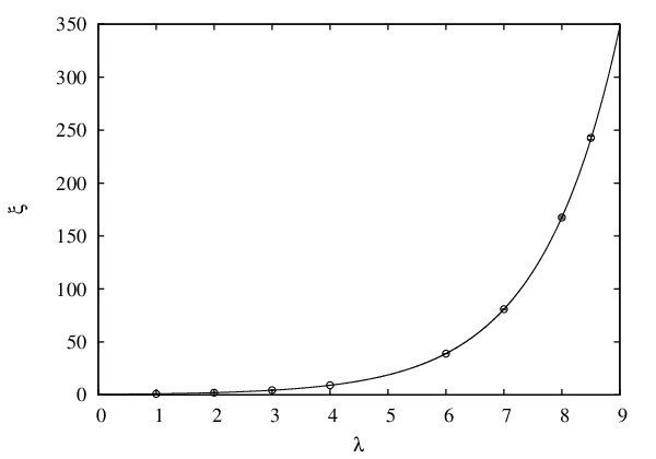
We now investigate the vortex suppression action without an angle constraint (which corresponds to ). Thus we consider the upper axis in the phase diagram of Figure 1. We have determined the infinite volume correlation length as a function of the vortex suppression parameter on lattice sizes up to . The results can be fitted well to the function
| (4.1) |
where and are fitting parameters, see Figure 6. This suggests that the critical value is at , as we anticipated in Figure 1. This limit can be viewed as a plaquette constraint action.
Studying the transition by measuring the step-2 SSF
| (4.2) |
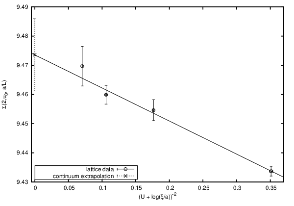
(cf. Subsection 3.2) confronts us with an additional limitation. The numerical results show that for this action the finite size effects constrain the finite volume correlation length to . This restricts the range of the variable to a regime .
A restriction of this kind is natural in models with discrete energy eigenvalues in a UV conformal limit [42].55 5 This is the ordinary case; asymptotically free theories (in the usual sense) are the exception, where any is possible. Also for the standard action in the 2d XY Model there is an upper bound
| (4.3) |
in the massive phase, see e.g. Ref. [41] and references therein. Qualitatively, such an upper bound can be understood using inequalities for ferromagnetic systems. This is briefly discussed in Appendix B.
We can still measure the step-2 SSF for sufficiently large, for instance , and try to fit the cut-off behaviour with the function from eq. (3.3), which describes the continuum limit at a BKT point. This fit, shown in Figure 7, works quite well. However, its continuum extrapolation , given in Table 6, is rather far from the analytic BKT value of [42] (which is close to ). This suggests that the endpoint of the transition line does not represent a BKT phase transition. Indeed, this point is specific in the sense that one cannot cross it (on the axis ). Moreover, this observation is fully consistent with the established pictures of vortices driving the BKT transition [15], so it cannot occur in the absence of vortices.
| d.o.f. | ||||
|---|---|---|---|---|
| 0.72 | 0.44(68) | 9.474(12) | 11.5314 |
In the 3d XY Model, the analogous point (, with no other restriction) has been studied in Ref. [43]. Also in that case the observation of the transverse susceptibility did not clarify the properties of this vortex-free case.
5 Concluding Discussion
In this paper, we have investigated topological lattice actions for the 2d XY Model. At the classical level, these actions do not define a proper field theory, and perturbation theory is not applicable.
In order to efficiently simulate topological actions, we have employed variants of the Wolff cluster algorithm. Its application to the constraint action is straightforward, and for the vortex suppression action a generalisation to 4-spin interactions has been developed and applied successfully, see Appendix A.
Despite its classical deficiencies, just as in the 2d Model, we found that — up to moderate vortex suppression — topological actions yield the correct quantum continuum limit, which is here associated with the BKT phase transition. This includes in particular topological actions where vortices do not cost any energy. This observation is remarkable in light of attempts to derive the critical line from the energy requirement for isolated vortices.
Specifically, in the massive phase, just as for the standard lattice action, the continuum limit is related to the sine-Gordon Model. In the massless phase we have verified the usual BKT behaviour of the critical exponent — and of its logarithmic correction term — with the topological actions. Our study demonstrates again the immense robustness of universality in quantum field theory, which does not rely on classical concepts.
An exception is the endpoint of this critical line, which seems to
be located at .
The extrapolation to this point — which represents a plaquette
constraint action — does not coincide with the BKT behaviour.
This agrees with the established picture that vortices (which are
completely eliminated at this point) are required to arrange for a
BKT transition [15].
For comparison, we mention the case of the so-called Extended XY Model, with the lattice action [44]
| (5.1) |
in the notation of eq. (2.1), and with . For it is equivalent to the standard action, but increasing leads to a more and more narrow potential well for , with width . The motivation was also an explicit vortex suppression; in the quadratic approximation to the potential they cost energy .
Due to the gradual suppression of the vortices for increasing exponents (even without fully excluding them), Ref. [44] predicted the phase transition to turn into first order above some value of , so it would match the behaviour which is observed experimentally for melting films of noble gases adsorbed on graphite.
This Extended XY Model has been investigated in numerous papers. The essential BKT phase transition is observed at low values of , and for some time the conjectured first order transition at large was controversial. However, it is now well confirmed numerically at [45, 46]. Moreover, an analytical proof for this conjecture was given in Ref. [47]. Ref. [48] added a vortex eliminating term with also in this case. No phase transition was observed at finite , hence the authors concluded that not only the BKT transition, but also the first order transition at large is driven by vortices.
In contrast, for the Step Model no non-BKT phase transition has ever been found, and for the topological lattice actions we do not observe any finite order transition in the - phase diagram either. However, a change to first order along the transition line — at some large value of — is conceivable in our case as well (that would not contradict universality). If this occurs as in the Extended XY Model, then it should change again at the endpoint, according to Ref. [48].
In any case, the characteristics of the transition at the vortex-free
endpoint is an open question, to be explored in the future.
Acknowledgements : We thank for very useful communications with J. Balog, E. Seiler, P. Weisz and U. Wolff. This work was supported in parts by the Schweizerischer Nationalfonds (SNF), and by the Consejo Nacional de Ciencia y Tecnología (CONACyT), project 155905/10 “Física de Partículas por medio de Simulaciones Numéricas”. The “Albert Einstein Center for Fundamental Physics” at Bern University is supported by the “Innovations- und Kooperationsprojekt C-13” of the Schweizerische Universitätskonferenz (SUK/CRUS).
Appendix A Cluster Algorithm for the Vortex Suppression Action
The algorithm for the vortex suppression angle constraint action is based on the Wolff cluster algorithm [3]. In the single cluster variant, each cluster update begins with the selection of an initial spin as a seed for cluster growth, and with the choice of a reflection line (a reflection hyper-plane in general Models), which is perpendicular to the randomly selected unit vector . Starting with this seed, some spins are combined to a cluster, which are then collectively reflected — or flipped — to the new spin orientations . Spins may be put in the same cluster due to the nearest-neighbour angle constraint, or due to the vortex suppression plaquette interaction. Two nearest-neighbour spins and are always put in the same cluster if the flip of to (without flipping ) would lead to a relative angle between and beyond the constraint angle .
The cluster rules implied by the vortex suppression four-spin plaquette action are more complicated. Let us consider the spins at the four corners , , and of a plaquette , as well as their reflection partners . Depending on whether a spin is flipped or not, there are 16 possible spin configurations on the given plaquette. Each one has a Boltzmann weight , depending on the vortex number of the corresponding spin configuration. Since the reflection of all four spins on a plaquette just changes the sign of the vortex charge , each of the 16 spin configurations has a total reflection partner with the same Boltzmann weight. We can thus limit the discussion to 8 pairs of configurations. We distinguish two qualitatively different cases:
- 1.
In this simple case the vortex number is always zero, irrespective of whether any spin is flipped or not. Hence all 16 spin configurations have the same Boltzmann weight 1. Based on the vortex suppression action, there is no need to put any of these four spins in a common cluster.
- 2.
The second case can be characterised as follows: when all spins are flipped to the same side of the reflection line, the vortex number is necessarily zero. We denote this spin configuration as the “reference configuration”. When each of the spins is individually flipped (without flipping any other spins), there are two spins whose flip generates a vortex (or an anti-vortex). We denote these two as the “active spins”. It turns out that the simultaneous flip of two spins (starting out of the reference configuration) generates a vortex only if exactly one of the two spins is active. If both or none of the two flipped spins are active, no vortex is generated. If three or four spins are flipped simultaneously, one just generates the total reflection partners of the previously discussed cases.
This gives rise to the following cluster formation rule. If the two active spins are on the same side of the reflection line, they are put into the same cluster with probability , otherwise they remain independent. The other spins are not affected by the vortex suppression action on this plaquette and remain independent. Still, preliminarily independent spins may finally become members of the cluster due to the angle constraint, or due to the vortex suppression action on a neighbouring plaquette.66 6 It should be noted that two active spins that are tied together in the same cluster may actually end up not to belong to the single cluster that is currently being built. In any case, one must keep track of the plaquettes on which a decision based on has already been taken, and one must stick to that decision when this plaquette is visited again, in the process of identifying the cluster members. For the efficiency of the algorithm it is essential that spins are put in the same cluster only if they are on the same side of the reflection line. This prevents the clusters from becoming unphysically large (their linear size should be of ).
This algorithm obeys detailed balance. In particular, when a plaquette carries a vortex (and thus has the Boltzmann weight ), the two active spins are not put in the same cluster (with probability ), because they are then necessarily on two different sides of the reflection line. On the other hand, if the two active spins are on the same side of the reflection line, and the Boltzmann weight is . In that case, the two active spins are put in the same cluster with probability , while they remain independent with probability . Only in the latter case, the two active spins may not belong to the same cluster, and are thus flipped independently, which again results in the creation of a vortex. Hence the detailed balance relation connecting the two configurations reads
(A.1)
As we have explicitly verified in an extensive computer search, other
cases do not exist. Once spins have been put together in the same cluster
(due to the nearest-neighbour angle constraint action, and/or due to the
vortex suppression plaquette interaction), all spins in the
cluster are simultaneously flipped to . Then a new random
site is selected as a seed for cluster growth, along with a new unit
vector , and the entire procedure is repeated.
As an alternative to this single-cluster algorithm, we also employed a multi-cluster algorithm, which constructs all clusters in a spin configuration and flips each of them with a probability of . Then the subtleties explained in footnote 6 do not occur.
An additional virtue of cluster algorithms is the applicability of improved estimators. For the variant that updates the vortex suppression angle constraint action, the improved estimators — for example for the correlation function and the susceptibility — work exactly as in the original Wolff algorithm [3].
Appendix B On Inequalities for Ferromagnetic Systems
Consider the standard action (2.1) on a long strip with sites on a time-slice. (We take below for simplicity.) Making the ferromagnetic coupling anisotropic, , we increase while keeping constant. This way the 2d system turns into a 1d chain with . By increasing a -parameter in a ferromagnetic system one might expect that the correlation length could only grow. This implies a lower bound for the correlation length in the original model (with isotropic coupling)
| (B.1) |
where is the correlation length for the 1d chain.
According to Ginibre’s Theorem [49] this intuitive argument indeed holds for the standard action, and for a large class
of further actions specified in Ref. [49].
Surprisingly, for slightly more complicated actions this inequality does not hold. Consider the nearest neighbour action with the action density
| (B.2) |
where the last term describes the constraint . One can make the system “more ferromagnetic” by increasing or , or by decreasing . Taking again the 1d limit (say, by ) one would naïvely expect
| (B.3) |
This, however, cannot be true, since one has for and for , while the left-hand-side increases in the massless phase. (Of course, the action (B.2) does not satisfy the conditions of Ginibre’s Theorem.)
In Table 7 we illustrate this behaviour for the mixed action (without the constraint, ), where the inequality is violated, and for the standard action (, ) where it holds.
References
- [2] W. Bietenholz, U. Gerber, M. Pepe and U.-J. Wiese, JHEP 1012 (2010) 020.
- [3] U. Wolff, Phys. Rev. Lett. 62 (1989) 361; Nucl. Phys. B 334 (1990) 581.
- [4] J. Balog and A. Hegedus, J. Phys. A: Math. Gen. 37 (2004) 1881.
- [5] M. Lüscher, P. Weisz and U. Wolff, Nucl. Phys. B 359 (1991) 221.
- [6] J. Balog, F. Niedermayer and P. Weisz, Phys. Lett. B 676 (2009) 188; Nucl. Phys. B 824 (2010) 563.
- [7] J. Balog, F. Niedermayer, M. Pepe, P. Weisz and U.-J. Wiese, arXiv:1208.6232 [hep-lat].
- [8] M. Lüscher, Commun. Math. Phys. 85 (1982) 29.
- [9] M. Bögli, F. Niedermayer, M. Pepe and U.-J. Wiese, JHEP 1204 (2012) 117.
- [10] D. Nogradi, JHEP 1205 (2012) 089.
- [11] P. de Forcrand, M. Pepe and U.-J. Wiese, Phys. Rev. D 86 (2012) 075006.
- [12] P. Minnhagen, Rev. Mod. Phys. 59 (1987) 1001.
- [13] S.L. Sondhi, S.M. Girvin, J.P. Carini and D. Shahar, Rev. Mod. Phys. 69 (1997) 315.
- [14] V.L. Berezinskii, Sov. Phys. JETP 32 (1970) 493.
- [15] J.M. Kosterlitz and D.J. Thouless, J. Phys. C6 (1973) 1181.
- [16] J. Balog, M. Niedermaier, F. Niedermayer, A. Patrascioiu, E. Seiler and P. Weisz, Nucl. Phys. B 618 (2001) 315.
- [17] J. Balog, F. Knechtli, T. Korzec and U. Wolff, Nucl. Phys. B 675 (2003) 555.
- [18] J. Balog, J. Phys. A 34 (2001) 5237.
- [19] A.J. Guttmann and G.S. Joice, J. Phys. C 6 (1973) 2691.
- [20] M.N. Barber, J. Phys. A 16 (1983) 4053.
- [21] A. Nymeyer, J. Phys. A 19 (1986) 2183.
- [22] E. Sánchez-Velasco and P. Wills, Phys. Rev. B 37 (1988) 406.
- [23] R. Kenna and A.C. Irving, Phys. Lett. B 351 (1995) 273; Nucl. Phys. B 485 (1997) 583. A.C. Irving and R. Kenna, Phys. Rev. B 53 (1996) 11568.
- [24] P. Olsson and P. Holme, Phys. Rev. B 63 (2001) 052407.
- [25] P. Minnhagen and B.J. Kim, Phys. Rev. B 67 (2003) 172509.
- [26] C. Destri and H.J. de Vega, Phys. Rev. Lett. 69 (1992) 2313; Nucl. Phys. B 504 (1997) 621.
- [27] G. Feverati, F. Ravanini and G. Takács, Phys. Lett. B 444 (1998) 442.
- [28] J.M. Kosterlitz, J. Phys. C 7 (1974) 1046.
- [29] J.V. José, L.P. Kadanoff, S. Kirkpatrick and D.R. Nelson, Phys. Rev. B 16 (1977) 1217.
- [30] G. Kohrig, R.E. Shrock and P. Wills, Phys. Rev. Lett. 57 (1986) 1358.
- [31] M.-h. Lau and C. Dasgupta, Phys. Rev. B 39 (1989) 7212.
- [32] J.F. Fernández, M.F. Ferreira and J. Stankiewicz, Phys. Rev. 34 (1986) 292.
- [33] A. Patrascioiu and E. Seiler, Phys. Rev. B 54 (1996) 7177.
- [34] M. Campostrini, A. Pelissetto, P. Rossi and E. Vicari, Phys. Rev. B 54 (1996) 7301.
- [35] W. Janke, Phys. Rev. B 55 (1997) 3580.
- [36] M. Hasenbusch and K. Pinn, J. Phys. A 30 (1997) 63.
- [37] A. Jaster and H. Hahn, Physica A 252 (1998) 199.
- [38] I. Dukovski, J. Machta and L. Chayes, Phys. Rev. E 65 (2002) 026702.
- [39] S. Chandrasekharan and C.G. Strouthas, Phys. Rev. D 68 (2003) 091502.
- [40] R. Kenna, arXiv:cond-mat/0512356 [cond-mat.stat-mech].
- [41] M. Hasenbusch, J. Phys. A 38 (2005) 5869.
- [42] J. Balog, private communication.
- [43] R. Fisch, Phys. Rev. B 52 (1995) 12512.
- [44] E. Domany, M. Schick and R.H. Swendsen, Phys. Rev. Lett. 52 (1984) 1535.
- [45] S. Ota and S.B. Ota, Phys. Lett. A 356 (2006) 393.
- [46] S. Sinha and S.K. Roy, Phys. Rev. E 81 (2010) 022102.
- [47] A.C.D. van Enter and S.B. Shlosman, Phys. Rev. Lett. 89 (2002) 285702.
- [48] S. Sinha and S.K. Roy, Phys. Rev. E 81 (2010) 041120.
- [49] J. Ginibre, Commun. Math. Phys. 16 (1970) 310.