跳到论文正文
W Papers独立论文阅读器 arXiv:1212.0499 论文正文 计算阅读时间 · 0%
引用这篇论文根据当前论文元数据生成,正式投稿前建议核对。


License: arXiv.org perpetual non-exclusive license
arXiv:1212.0499v4 [math.AP] 07 Dec 2012

A Note on Semi-linear Wave Equations

Shuang Miao
Abstract

Inspired by the work of Wang and Yu [21] on wave maps, we show that for all positive numbers T0>0T_{0}>0 and E0>0E_{0}>0, a large kind of semi-linear wave equation on ℝ×ℝ3\mathbb{R}\times\mathbb{R}^{3} has a solution whose life-span is [0,T0][0,T_{0}], and the energy of the initial Cauchy data is at least E0E_{0}.

1 Introduction

We consider in ℝ×ℝ3\mathbb{R}\times\mathbb{R}^{3} the equation:

□​ϕ=±|ϕ|k−1​ϕ\displaystyle\Box\phi=\pm|\phi|^{k-1}\phi (1)

where

□=−∂t​t2+Δx,\displaystyle\Box=-\partial_{tt}^{2}+\Delta_{x},

and kk is a odd number satisfying k≥3k\geq 311 1 In this case, small data generates global solution, see [7]. And we shall see that to establish the main estimates, we only need the nonlinearity to be a smooth function of ϕ\phi which vanishes at the origin and whose growth is at least |ϕ|2|\phi|^{2} when |ϕ||\phi| is large.. The equation (1) has a conserved energy

E⁡(ϕ⁡(t))=12​∫ℝ3|∂tϕ⁡(t,x)|2+|∇xϕ​(t,x)|2±2k+1​|ϕ⁡(t,x)|k+1​𝑑x\displaystyle E(\phi(t))=\frac{1}{2}\int_{\mathbb{R}^{3}}|\partial_{t}\phi(t,x)|^{2}+|\nabla_{x}\phi(t,x)|^{2}\pm\frac{2}{k+1}|\phi(t,x)|^{k+1}dx (2)

The equation (1) is called defocusing, if there is a plus sign in front of the nonlinearity, otherwise it is called focusing. In view of the Sobolev embedding H1​(ℝ3)↪L6​(ℝ3)H^{1}(\mathbb{R}^{3})\hookrightarrow L^{6}(\mathbb{R}^{3}), one refers to the range k<5k<5 as the energy-subcritical regime, to k=5k=5 as the energy-critical regime and to k>5k>5 as the energy-supercritical regime. So the super-critical wave equations (k>5k>5) (both defocusing and focusing case) are included in our present note.

The study of the Cauchy problem for (1) has a long history. For the defocusing case, Rauch [13] showed global existence for arbitrary smooth data for subcritical equations and for small energy smooth data in the critical case. Struwe [16] obtained global existence for large but radially symmetric data in the critical case, then Grillakis [5] removed the radially symmetric condition on the data. After that Shatah and Struwe [15] studied the energy-class solutions. See also [1], [2] and [18] for further results. The study of focusing case is initiated by Krieger and Schlag [12] as well as Kenig and Merle [8]. Up to now, only a few results are known about the energy-supercritical case. See [9], [10] and [19].

Inspired by the recent work [21], we study long time solutions of semi-linear wave equations by a different approach. Following the “short-pulse” method, which was first introduced by Christodoulou [3], and extended by Klainerman and Rodnianski [11], we establish the following long-time existence result for equation (1):

Main Theorem For any T0>0T_{0}>0 and E0>0E_{0}>0, there exist (ϕ0,ϕ1)∈C∞​(ℝ3)×C∞​(ℝ3)(\phi_{0},\phi_{1})\in C^{\infty}(\mathbb{R}^{3})\times C^{\infty}(\mathbb{R}^{3}) such that the Cauchy problem for (1) with initial data (ϕ,ϕt)|t=0=(ϕ0,ϕ1)(\phi,\phi_{t})|_{t=0}=(\phi_{0},\phi_{1}) has a unique solution ϕ∈C∞​([0,T0]×ℝ3)\phi\in C^{\infty}([0,T_{0}]\times\mathbb{R}^{3}) with energy of at least E0E_{0}.

In [21], Wang and Yu constructed a solution for 2+1 wave maps with 𝕊2\mathbb{S}^{2} as its target, by using a bootstrap argument. Since the characteristic initial data (so called s​h​o​r​t​p​u​l​s​eshortpulse) is chosen to be highly-oscillating, they can close the bootstrap. Then the solution will automatically have a life-span [0,T0][0,T_{0}], where T0T_{0} is an arbitrary positive number given priorly. If the initial data is chosen properly, then the initial energy will be at least E0E_{0}, where E0E_{0} is also an arbitrary positive number given priorly. The crucial point in their work is that the nonlinearity of wave maps into 𝕊2\mathbb{S}^{2} is a “null form”, this means that the nonlinearity is “not too bad”, so that they can absorb the term original from the nonlinearity in the a priori estimates if the characteristic initial data oscillates heavily enough. Wang and Yu also studied the 3+1 nonlinear wave equation with a “null form” by choosing the initial data at past null infinity, so they can even obtain global existence for large energy data, see [20].

In the current work, there are no “null form” in the nonlinearity, but instead, the nonlinearity depends only on the solution itself, and we only commute the “bad” vectorfield once with the operator □\Box when we do the bootstrap argument, so the nonlinearity will not cause trouble. Moreover, since the nonlinearity involves only the solution itself, we need one derivative less to close the bootstrap than the work of Wang and Yu. Our method for 3+1 semi-linear wave equations is also valid in the 2+1 case, and we shall talk about this briefly at the end of the paper.

2 Preliminaries

2.1 Basic Geometric Construction

This part is quite similar to [21], the only difference is that we are in the 3-space dimensional Minkowski spacetime ℝ×ℝ3\mathbb{R}\times\mathbb{R}^{3}. We shall use the same notations as in [21]. We have the optical functions:

u=12​(t−r)u¯=12​(t+r)\displaystyle u=\frac{1}{2}(t-r)\quad\underline{u}=\frac{1}{2}(t+r)

null vectorfields:

L=∂t+∂rL¯=∂t−∂r\displaystyle L=\partial_{t}+\partial_{r}\quad\underline{L}=\partial_{t}-\partial_{r}

as well as the rotation fields:

Ωi​j=xi∂j−xj∂i,1≤i,j≤3\displaystyle\Omega_{ij}=x_{i}\partial_{j}-x_{j}\partial_{i},1\leq i,j\leq 3

and also the relation between the operators Ω\Omega and ∇̸\not{\nabla}:

|Ωk​ϕ|=|r|k​|∇̸kϕ|\displaystyle|\Omega^{k}\phi|=|r|^{k}|\not{\nabla}^{k}\phi| (3)

In section 3 and section 4, the parameter uu will be confined in the interval [u0,−1][u_{0},-1] where u0∼−T0u_{0}\sim-T_{0} (then we can see that the life-span will be automatically ∼T0\sim T_{0}). The parameter u¯\underline{u} is confined in [0,δ][0,\delta] where δ\delta is a small parameter which will be determined later. As in [21], the corresponding cones are pictured as follows (See 1).

Refer to caption
Figure 1: null cones (This figure is borrowed from [21].)

When we derive estimates in section 3 and 4, u¯∈[0,δ]\underline{u}\in[0,\delta] where δ\delta will be sufficiently small. Since T0T_{0} and u0u_{0} are fixed numbers, in the region where (u¯,u]∈[0,δ]×[u0,−1](\underline{u},u]\in[0,\delta]\times[u_{0},-1], the parameter r∼1r\sim 1. In particular, we have

|Ωk​ϕ|∼|∇̸kϕ|\displaystyle|\Omega^{k}\phi|\sim|\not{\nabla}^{k}\phi|

2.2 Energy Identity

Let ff be a solution for the following non-homogenous wave equation on ℝ3+1\mathbb{R}^{3+1}:

□​f=Φ\displaystyle\Box f=\Phi (4)

The energy momentum tensor associated to ff is

Tμ​ν​[f]=∂μf​∂νf−12​gμ​ν​|∇f|2\displaystyle T_{\mu\nu}[f]=\partial_{\mu}f\partial_{\nu}f-\frac{1}{2}g_{\mu\nu}|\nabla f|^{2} (5)

Obviously, it is symmetric and satisfies the following identity:

∇μTμ​ν​[f]=Φ⋅∇νf\displaystyle\nabla^{\mu}T_{\mu\nu}[f]=\Phi\cdot\nabla_{\nu}f (6)

Given a vectorfield XX, which will be used as a m​u​l​t​i​p​l​i​e​rmultiplier v​e​c​t​o​r​f​i​e​l​dvectorfield, the associated energy currents are defined as follows

PαX​[f]=Tα​μ​[f]​Xμ,KX​[f]=12​Tμ​ν​[f](X)​πμ​ν\displaystyle P^{X}_{\alpha}[f]=T_{\alpha\mu}[f]X^{\mu},\quad K^{X}[f]=\frac{1}{2}T^{\mu\nu}[f]{\vphantom{\pi}}^{(X)}{\pi}_{\mu\nu}

where the deformation tensor πμ​ν(X){\vphantom{\pi}}{}^{(X)}{\pi}_{\mu\nu} is defined by

πμ​ν(X)=ℒX​gμ​ν=∇μXν+∇νXμ{\vphantom{\pi}}{}^{(X)}{\pi}_{\mu\nu}=\mathcal{L}_{X}g_{\mu\nu}=\nabla_{\mu}X_{\nu}+\nabla_{\nu}X_{\mu} (7)

By (6), we easily obtain:

∇μPμX​[f]=KX​[f]+Φ⋅X​f\displaystyle\nabla^{\mu}P^{X}_{\mu}[f]=K^{X}[f]+\Phi\cdot Xf (8)

We can express TT in terms of null frames {e1=r−1∂θ,e2=(rsinθ)−1,e3=L¯,e4=L}\{e_{1}=r^{-1}\partial_{\theta},e_{2}=(r\sin\theta)^{-1},e_{3}=\underline{L},e_{4}=L\}:

T⁡(L,L)=|L​f|2T⁡(L¯,L¯)=|L¯​f|2T⁡(L,L¯)=|∇̸f|2\displaystyle T(L,L)=|Lf|^{2}\quad T(\underline{L},\underline{L})=|\underline{L}f|^{2}\quad T(L,\underline{L})=|\not{\nabla}f|^{2}

where we express the Minkowski metric in polar coordinates:

g=−d​t2+d​r2+r2​(d​θ2+(sin⁡θ)2​d​φ2)\displaystyle g=-dt^{2}+dr^{2}+r^{2}(d\theta^{2}+(\sin\theta)^{2}d\varphi^{2})

We shall use X=LX=L and L¯\underline{L} as multiplier vectorfields, the corresponding deformation tensors and currents are:

(L)π=1rg̸(L¯)π=−1rg̸{\vphantom{\pi}}{}^{(L)}{\pi}=\frac{1}{r}\not{g}\quad{\vphantom{\pi}}^{(\underline{L})}{\pi}=-\frac{1}{r}\not{g} (9)
KL=12​r​L​f​L¯​f,KL¯=−12​r​L​f​L¯​f\displaystyle\quad K^{L}=\frac{1}{2r}Lf\underline{L}f,\quad K^{\underline{L}}=-\frac{1}{2r}Lf\underline{L}f

where g̸\not{g} is the restriction of the Minkowski metric to the sphere Su¯,uS_{\underline{u},u}.

Refer to caption
Figure 2: integral domain (This figure is borrowed from [21].)

We use 𝒟⁡(u,u¯)\mathcal{D}(u,\underline{u}) to denote the space-time slab enclosed by the hypersurfaces Cu0C_{u_{0}}, C¯0\underline{C}_{0}, CuC_{u} and C¯u¯\underline{C}_{\underline{u}} as pictured above (see 2). We integrate (8) on 𝒟⁡(u,u¯)\mathcal{D}(u,\underline{u}) to obtain:

∫CuT⁡[f]​(X,L)+∫C¯u¯T⁡[f]​(X,L¯)=∫Cu0T⁡[f]​(X,L)+∫C¯0T⁡[f]​(X,L¯)\displaystyle\int_{C_{u}}T[f](X,L)+\int_{\underline{C}_{\underline{u}}}T[f](X,\underline{L})=\int_{C_{u_{0}}}T[f](X,L)+\int_{\underline{C}_{0}}T[f](X,\underline{L})
+∬𝒟⁡(u,u¯)KX[f]+Φ⋅Xf\displaystyle+\iint_{\mathcal{D}(u,\underline{u})}K^{X}[f]+\Phi\cdot Xf

where LL and L¯\underline{L} are corresponding normals of the null hypersurfaces CuC_{u} and C¯u¯\underline{C}_{\underline{u}}.

In applications, the data on C¯0\underline{C}_{0} is always vanishing, thus, we have the following formula:

∫CuT⁡[f]​(X,L)+∫C¯u¯T⁡[f]​(X,L¯)=∫Cu0T⁡[f]​(X,L)+∬𝒟⁡(u,u¯)KX​[f]+Φ⋅X​f\displaystyle\int_{C_{u}}T[f](X,L)+\int_{\underline{C}_{\underline{u}}}T[f](X,\underline{L})=\int_{C_{u_{0}}}T[f](X,L)+\iint_{\mathcal{D}(u,\underline{u})}K^{X}[f]+\Phi\cdot Xf (10)

2.3 Gronwall and Sobolev Inequalities

We need the following Sobolev inequalities which can be derived from i​s​o​p​e​r​i​m​e​t​r​i​cisoperimetric i​n​e​q​u​a​l​t​yinequalty. The proof can be found in [3].

Lemma 2.1 Let (S,g̸)(S,\not{g}) be a compact 2-dimensional Riemannian manifold and ϕ\phi a smooth function on SS, which is square-integrable and with square-integrable first derivatives. Then for 2<p<∞2<p<\infty, ϕ∈Lp​(S)\phi\in L^{p}(S) and we have:

|S|−1/p∥ϕ∥Lp​(S)≤CpI′​(S)∥ϕ∥W12​(S)\displaystyle|S|^{-1/p}\|\phi\|_{L^{p}(S)}\leq C_{p}\sqrt{I^{\prime}(S)}\|\phi\|_{W^{2}_{1}(S)}

Here CpC_{p} is a numerical constant depending only on pp, and |S||S| is the area of the sphere Su¯,uS_{\underline{u},u}.

I′​(S)=max⁡{I⁡(S),1}\displaystyle I^{\prime}(S)=\max\{I(S),1\}

where I⁡(S)I(S) is the isoperimetric constant of SS, and we define:

∥ϕ∥W12​(S)=∥∇̸ϕ∥L2​(S)+|S|−1/2∥ϕ∥L2​(S)\displaystyle\|\phi\|_{W^{2}_{1}(S)}=\|\not{\nabla}\phi\|_{L^{2}(S)}+|S|^{-1/2}\|\phi\|_{L^{2}(S)}

Lemma 2.2 Let (S,g̸)(S,\not{g}) be a compact 2-dimensional Riemannian manifold and ϕ\phi a smooth function on SS, which belongs to Lp​(S)L^{p}(S) and with first derivatives which also belong to Lp​(S)L^{p}(S), for some p>2p>2. Then ϕ∈L∞​(S)\phi\in L^{\infty}(S) and we have

sup|ϕ|≤Cp​I′​(S)​|S|(1/2)−(1/p)​‖ϕ‖W1p​(S)\displaystyle\sup|\phi|\leq C_{p}\sqrt{I^{\prime}(S)}|S|^{(1/2)-(1/p)}\|\phi\|_{W^{p}_{1}(S)}

Here CpC_{p} is a numerical constant depending only on pp, and we define:

∥ϕ∥W1p​(S)=∥∇̸ϕ∥Lp​(S)+|S|−1/2∥ϕ∥Lp​(S)\displaystyle\|\phi\|_{W^{p}_{1}(S)}=\|\not{\nabla}\phi\|_{L^{p}(S)}+|S|^{-1/2}\|\phi\|_{L^{p}(S)}

Also by i​s​o​p​e​r​i​m​e​t​r​i​cisoperimetric i​n​e​q​u​a​l​i​t​yinequality, we can deduce:

Lemma 2.3 Let ϕ\phi be a smooth function on CuC_{u} vanishing on S0,uS_{0,u} then with the same condition as Lemma 2.1, we have:

∫Su¯,u|ϕ|6​d​μg̸≤C⁡(∫Su¯,u|ϕ|4​d​μg̸)​(|u|−2​∫Su¯,u|ϕ|2​d​μg̸+∫Su¯,u|∇̸ϕ|2​d​μg̸)\displaystyle\int_{S_{\underline{u},u}}|\phi|^{6}d\mu_{\not{g}}\leq C(\int_{S_{\underline{u},u}}|\phi|^{4}d\mu_{\not{g}})(|u|^{-2}\int_{S_{\underline{u},u}}|\phi|^{2}d\mu_{\not{g}}+\int_{S_{\underline{u},u}}|\not{\nabla}\phi|^{2}d\mu_{\not{g}})

where CC is an absolute constant.

Obviously, from Lemma 2.1 and Lemma 2.2, we obtain:

supS|ϕ|≤Cp[|S|−1/2∥ϕ∥L2​(S)+∥∇̸ϕ∥L2​(S)+|S|1/2∥∇̸2ϕ∥L2​(S)]\displaystyle\sup_{S}|\phi|\leq C_{p}[|S|^{-1/2}\|\phi\|_{L^{2}(S)}+\|\not{\nabla}\phi\|_{L^{2}(S)}+|S|^{1/2}\|\not{\nabla}^{2}\phi\|_{L^{2}(S)}] (11)

With the same condition as Lemma 2.3, we have:

Lemma 2.4 Let ϕ\phi be a smooth CuC_{u}-function vanishing on C¯0\underline{C}_{0}, we have:

supu¯(|u|1/2​‖ϕ‖L4​(Su¯,u))≤Cp​‖L​ϕ‖L2​(Cu)1/2​[‖ϕ‖L2​(Cu)+|u|​‖∇̸ϕ‖L2​(Cu)]1/2\displaystyle\sup_{\underline{u}}(|u|^{1/2}\|\phi\|_{L^{4}(S_{\underline{u},u})})\leq C_{p}\|L\phi\|^{1/2}_{L^{2}(C_{u})}[\|\phi\|_{L^{2}(C_{u})}+|u|\|\not{\nabla}\phi\|_{L^{2}(C_{u})}]^{1/2}

and by Gronwall’s inequality, we have:

‖ϕ‖L2​(Su¯,u)≲‖L​ϕ‖L2​(Cu)1/2​‖ϕ‖L2​(Cu)1/2\displaystyle\|\phi\|_{L^{2}(S_{\underline{u},u})}\lesssim\|L\phi\|^{1/2}_{L^{2}(C_{u})}\|\phi\|^{1/2}_{L^{2}(C_{u})}

Also from Lemma 2.3, we have:

Lemma 2.5 Let ϕ\phi be a smooth function on C¯u¯\underline{C}_{\underline{u}}, the following estimates hold:

supu(|u|1/2∥ϕ∥L4​(Su¯,u))≤Cp{|u0|1/2∥ϕ∥L4​(Su¯,u0)+∥|u|1/2L¯ϕ∥L2​(C¯u¯)1/2⋅\displaystyle\sup_{u}(|u|^{1/2}\|\phi\|_{L^{4}(S_{\underline{u},u})})\leq C_{p}\{|u_{0}|^{1/2}\|\phi\|_{L^{4}(S_{\underline{u},u_{0}})}+\||u|^{1/2}\underline{L}\phi\|^{1/2}_{L^{2}(\underline{C}_{\underline{u}})}\cdot
[∥|u|−1/2ϕ∥L2​(C¯u¯)2+∥|u|1/2∇̸ϕ∥L2​(C¯u¯)2]1/4}\displaystyle\ [\||u|^{-1/2}\phi\|_{L^{2}(\underline{C}_{\underline{u}})}^{2}+\||u|^{1/2}\not{\nabla}\phi\|^{2}_{L^{2}(\underline{C}_{\underline{u}})}]^{1/4}\}

also:

‖ϕ‖L2​(Su¯,u)≲‖ϕ‖L2​(Su¯,u0)+‖L¯​ϕ‖L2​(C¯u¯)1/2​‖ϕ‖L2​(C¯u¯)1/2\displaystyle\|\phi\|_{L^{2}(S_{\underline{u},u})}\lesssim\|\phi\|_{L^{2}(S_{\underline{u},u_{0}})}+\|\underline{L}\phi\|^{1/2}_{L^{2}(\underline{C}_{\underline{u}})}\|\phi\|^{1/2}_{L^{2}(\underline{C}_{\underline{u}})}

From the above lemmas, we can easily obtain the following L∞L^{\infty} estimates:

∥ϕ∥L∞​(Su¯,u)≲|u|−1/2∥Lϕ∥L2​(Cu)1/2∥ϕ∥1/2L2​(Cu)\displaystyle\|\phi\|_{L^{\infty}(S_{\underline{u},u})}\lesssim|u|^{-1/2}\|L\phi\|_{L^{2}(C_{u})}^{1/2}\|\phi\|^{1/2}_{L^{2}(C_{u})}
+∥L∇̸ϕ∥L2​(Cu)1/2∥∇̸ϕ∥L2​(Cu)1/2+|u|1/2∥L∇̸2ϕ∥L2​(Cu)1/2∥∇̸2ϕ∥L2​(Cu)1/2\displaystyle+\|L\not{\nabla}\phi\|_{L^{2}(C_{u})}^{1/2}\|\not{\nabla}\phi\|_{L^{2}(C_{u})}^{1/2}+|u|^{1/2}\|L\not{\nabla}^{2}\phi\|_{L^{2}(C_{u})}^{1/2}\|\not{\nabla}^{2}\phi\|_{L^{2}(C_{u})}^{1/2}

and also:

∥ϕ∥L∞​(Su¯,u)≲|u|−1/2∥ϕ∥L2​(Su¯,u0)+∥∇̸ϕ∥L2​(Su¯,u0)+|u|1/2∥∇̸2ϕ∥L2​(Su¯,u0)\displaystyle\|\phi\|_{L^{\infty}(S_{\underline{u},u})}\lesssim|u|^{-1/2}\|\phi\|_{L^{2}(S_{\underline{u},u_{0}})}+\|\not{\nabla}\phi\|_{L^{2}(S_{\underline{u},u_{0}})}+|u|^{1/2}\|\not{\nabla}^{2}\phi\|_{L^{2}(S_{\underline{u},u_{0}})}
+|u|−1/2∥L¯ϕ∥L2​(C¯u¯)1/2∥ϕ∥1/2L2​(C¯u¯)+∥L¯∇̸ϕ∥L2​(C¯u¯)1/2∥∇̸ϕ∥L2​(C¯u¯)1/2+|u|1/2∥L¯∇̸2ϕ∥L¯2​(C¯u¯)1/2∥∇̸2ϕ∥L2​(C¯u¯)1/2\displaystyle+|u|^{-1/2}\|\underline{L}\phi\|_{L^{2}(\underline{C}_{\underline{u}})}^{1/2}\|\phi\|^{1/2}_{L^{2}(\underline{C}_{\underline{u}})}+\|\underline{L}\not{\nabla}\phi\|_{L^{2}(\underline{C}_{\underline{u}})}^{1/2}\|\not{\nabla}\phi\|_{L^{2}(\underline{C}_{\underline{u}})}^{1/2}+|u|^{1/2}\|\underline{L}\not{\nabla}^{2}\phi\|_{\underline{L}^{2}(\underline{C}_{\underline{u}})}^{1/2}\|\not{\nabla}^{2}\phi\|_{L^{2}(\underline{C}_{\underline{u}})}^{1/2}

In all of the above lemmas, we always assume that ϕ\phi vanishes on C¯0\underline{C}_{0}.

Actually, in the following, we only use another version of the above Sobolev inequality, with ∇̸\not{\nabla} substituted by Ω\Omega. In this case, the weight of |u||u| will change, but it doesn’t matter, because in our case, |u||u| is more or less like a constant.

We also need the standard Gronwall’s inequality:

Lemma 2.6 Let f⁡(t)f(t) be a non-negative function defined on an interval II with initial point t0t_{0}. If ff satisfies:

dd​t​f≤a⋅f+b\displaystyle\frac{d}{dt}f\leq a\cdot f+b

where two non-negative functions a,b∈L1​(I)a,b\in L^{1}(I), then for all t∈It\in I, we have:

f⁡(t)≤eA⁡(t)​(f⁡(t0)+∫t0te−A⁡(τ)​b​(τ)​𝑑τ)\displaystyle f(t)\leq e^{A(t)}(f(t_{0})+\int_{t_{0}}^{t}e^{-A(\tau)}b(\tau)d\tau) (12)

where A⁡(t)=∫t0ta⁡(τ)​𝑑τA(t)=\int_{t_{0}}^{t}a(\tau)d\tau.

2.4 Outline of the Proof

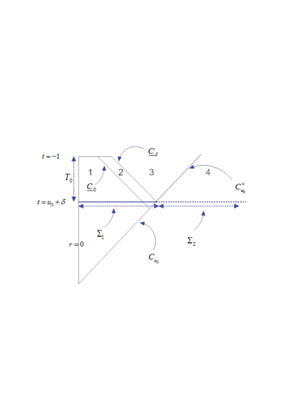
We will follow the main steps of [21]. The Cauchy data will be finally given on t=u0+δt=u_{0}+\delta and the solution will exist at least for t∈[u0+δ,−1]t\in[u_{0}+\delta,-1]. This can be shown in the above picture (see 3):

Refer to caption
Figure 3: construction of initial data (This figure is borrowed from [21].)

First, we give initial data on the null hypersurface Cu0C_{u_{0}} where u0≤u¯≤δu_{0}\leq\underline{u}\leq\delta. When u0≤u¯≤0u_{0}\leq\underline{u}\leq 0, the data is trivial, therefore the solution in Region 1 is zero. When 0≤u¯≤δ0\leq\underline{u}\leq\delta, the data will be chosen as follows:

ϕ⁡(u¯,u0,θ)=δ1/2​ψ0​(u¯δ,θ)\displaystyle\phi(\underline{u},u_{0},\theta)=\delta^{1/2}\psi_{0}(\frac{\underline{u}}{\delta},\theta)

where the energy of ψ0\psi_{0} is larger than E0E_{0}. We then show that we can construct a solution in Region 2. Consequently, we take the restriction of the solution constructed to the surface Σ1⊂{t=u0+δ}\Sigma_{1}\subset\{t=u_{0}+\delta\} as the first part of the Cauchy data.

Second, we extend the Cauchy data on Σ1\Sigma_{1} to Σ2⊂{t=u0+δ}\Sigma_{2}\subset\{t=u_{0}+\delta\} such that the energy is small. By small data theory, we can construct a solution in Region 4.

Third, From previous two steps, we can show that the restriction of the solution already constructed to C¯δ\underline{C}_{\delta} and Cu0+C^{+}_{u_{0}} (where u¯≥δ\underline{u}\geq\delta) are small. We use them as initial data and we can solve this small data problem to construct solution on Region 3. We finally combines the solutions in Region 1,2,3 and 4 to finish the construction.

3 Characteristic Initial Data

First, we require that the data ϕ⁡(u¯,u0,θ)\phi(\underline{u},u_{0},\theta) to satisfy

ϕ⁡(u¯,u0,θ)=0for allu¯≤0\displaystyle\phi(\underline{u},u_{0},\theta)=0\quad\textrm{for all}\quad\underline{u}\leq 0

Therefore, according to the Huygens principle, the solution ϕ\phi of (1) satisfies

ϕ≡0in Region 1={u¯(x)≤0,u0≤u(x)≤0}\displaystyle\phi\equiv 0\quad\textrm{in Region 1}\quad=\{\underline{u}(x)\leq 0,u_{0}\leq u(x)\leq 0\}

Secondly, we choose

ϕ⁡(u¯,u0,θ)=δ1/2​ψ0​(u¯δ,θ)\displaystyle\phi(\underline{u},u_{0},\theta)=\delta^{1/2}\psi_{0}(\frac{\underline{u}}{\delta},\theta) (13)

where ψ0\psi_{0} is a smooth function supported in (0,1)(0,1) with respect to its first variable.

The data given in the above form is called a s​h​o​r​tshort p​u​l​s​epulse, a name invented by Christodoulou in [3].

In order to derive the energy estimates, as in [21], we need the following commutators:

[L,Ω]=0[L¯,Ω]=0[□,Ω]=0\displaystyle[L,\Omega]=0\quad[\underline{L},\Omega]=0\quad[\Box,\Omega]=0 (14)
[□,L]=1r2​(L−L¯)+2r3​Δ̸[□,L¯]=1r2​(L¯−L)−2r3​Δ̸\displaystyle[\Box,L]=\frac{1}{r^{2}}(L-\underline{L})+\frac{2}{r^{3}}\not{\Delta}\quad[\Box,\underline{L}]=\frac{1}{r^{2}}(\underline{L}-L)-\frac{2}{r^{3}}\not{\Delta}

Here the operator Δ̸\not{\Delta} is the Laplacian on standard sphere 𝕊2\mathbb{S}^{2}.

On the initial hypersurface Cu0C_{u_{0}}, we have the following bounds on data:

∥Lϕ∥L∞​(Cu0)≲δ−1/2∥Ωϕ∥L∞​(Cu0)≲δ1/2\displaystyle\|L\phi\|_{L^{\infty}(C_{u_{0}})}\lesssim\delta^{-1/2}\quad\|\Omega\phi\|_{L^{\infty}(C_{u_{0}})}\lesssim\delta^{1/2}

and for higher order derivatives, we have:

∥LΩkϕ∥L∞​(Cu0)≲kδ−1/2\displaystyle\|L\Omega^{k}\phi\|_{L^{\infty}(C_{u_{0}})}\lesssim_{k}\delta^{-1/2}
∥Ωk+1ϕ∥L∞​(Cu0)≲kδ1/2\displaystyle\|\Omega^{k+1}\phi\|_{L^{\infty}(C_{u_{0}})}\lesssim_{k}\delta^{1/2}
∥L2Ωk−1ϕ∥L∞​(Cu0)≲kδ−3/2\displaystyle\|L^{2}\Omega^{k-1}\phi\|_{L^{\infty}(C_{u_{0}})}\lesssim_{k}\delta^{-3/2}

We also need a bound for L¯\underline{L}-derivatives. To do this, we write the equation in null frames:

−L​L¯​ϕ+1r2​Δ̸​ϕ+1r​(L​ϕ−L¯​ϕ)=±|ϕ|k−1​ϕ\displaystyle-L\underline{L}\phi+\frac{1}{r^{2}}\not{\Delta}\phi+\frac{1}{r}(L\phi-\underline{L}\phi)=\pm|\phi|^{k-1}\phi (15)

We can write the above as a propagation equation for L¯​ϕ\underline{L}\phi along Cu0C_{u_{0}}:

L⁡(L¯​ϕ)=a⋅L¯​ϕ+b\displaystyle L(\underline{L}\phi)=a\cdot\underline{L}\phi+b

where

a=−1rb=1r​L​ϕ+1r2​Δ̸​ϕ∓|ϕ|k−1​ϕ\displaystyle a=-\frac{1}{r}\quad b=\frac{1}{r}L\phi+\frac{1}{r^{2}}\not{\Delta}\phi\mp|\phi|^{k-1}\phi

Obviously,

∥a∥L∞​(Cu0)≲1,∥b∥L∞​(Cu0)≲δ−1/2\displaystyle\|a\|_{L^{\infty}(C_{u_{0}})}\lesssim 1,\quad\|b\|_{L^{\infty}(C_{u_{0}})}\lesssim\delta^{-1/2}

Then by Gronwall’s inequality, we easily obtain:

‖L¯​ϕ‖L∞​(Cu0)≲δ1/2\displaystyle\|\underline{L}\phi\|_{L^{\infty}(C_{u_{0}})}\lesssim\delta^{1/2} (16)

Similarly, by using the commutator, we obtain

‖L¯​Ω​ϕ‖L∞​(Cu0)≲δ1/2‖L¯​Ω2​ϕ‖L∞​(Cu0)≲δ1/2\displaystyle\|\underline{L}\Omega\phi\|_{L^{\infty}(C_{u_{0}})}\lesssim\delta^{1/2}\quad\|\underline{L}\Omega^{2}\phi\|_{L^{\infty}(C_{u_{0}})}\lesssim\delta^{1/2} (17)

To obtain a long time existence theorem for (1), we have to derive estimates on ϕ\phi as well as its derivatives. it’s very natual that these estimates should be compatible with the bounds for ϕ\phi on initial hypersurface. However, as stated in [21], a r​e​l​a​x​e​drelaxed estimate, which is easier to derive, is enough. That is, we just need the following bounds on Ωk​ϕ\Omega^{k}\phi:

∥Ωk+1ϕ∥L∞​(Cu0)≲k1\displaystyle\|\Omega^{k+1}\phi\|_{L^{\infty}(C_{u_{0}})}\lesssim_{k}1 (18)

Summarizing, we have the following bounds on initial data:

∥LΩkϕ∥L∞​(Cu0)≲δ−1/2\displaystyle\|L\Omega^{k}\phi\|_{L^{\infty}(C_{u_{0}})}\lesssim\delta^{-1/2} (19)
‖Ωk+1​ϕ‖L∞​(Cu0)≲1\displaystyle\|\Omega^{k+1}\phi\|_{L^{\infty}(C_{u_{0}})}\lesssim 1
‖L¯​Ωk​ϕ‖L∞​(Cu0)≲δ1/2\displaystyle\|\underline{L}\Omega^{k}\phi\|_{L^{\infty}(C_{u_{0}})}\lesssim\delta^{1/2}

for k=0,1,2k=0,1,2, and

∥L2ϕ∥L∞​(Cu0)≲δ−3/2\displaystyle\|L^{2}\phi\|_{L^{\infty}(C_{u_{0}})}\lesssim\delta^{-3/2} (20)
∥L2Ωϕ∥L∞​(Cu0)≲δ−3/2\displaystyle\|L^{2}\Omega\phi\|_{L^{\infty}(C_{u_{0}})}\lesssim\delta^{-3/2}

From these L∞L^{\infty} bounds, we obtain easily the L2L^{2} bounds:

‖L​Ωk​ϕ‖L2​(Cu0)≲1\displaystyle\|L\Omega^{k}\phi\|_{L^{2}(C_{u_{0}})}\lesssim 1 (21)
‖Ωk+1​ϕ‖L2​(Cu0)≲δ1/2\displaystyle\|\Omega^{k+1}\phi\|_{L^{2}(C_{u_{0}})}\lesssim\delta^{1/2}

for k=0,1,2k=0,1,2, and

‖L2​ϕ‖L2​(Cu0)≲δ−1\displaystyle\|L^{2}\phi\|_{L^{2}(C_{u_{0}})}\lesssim\delta^{-1} (22)
‖L2​Ω​ϕ‖L2​(Cu0)≲δ−1\displaystyle\|L^{2}\Omega\phi\|_{L^{2}(C_{u_{0}})}\lesssim\delta^{-1}

We shall show that (21) and (22) will hold on all later outgoing null hypersurfaces CuC_{u} where −1>u>u0-1>u>u_{0} provided the solution of (1) can be constructed up to CuC_{u}.

4 A priori Estimates

We start by defining a family of energy norms. For this purpose, we slightly abuse the notations: we use CuC_{u} to denote Cu[0,u¯]C^{[0,\underline{u}]}_{u} and C¯u¯\underline{C}_{\underline{u}} to denote C¯u¯[u0,u]\underline{C}_{\underline{u}}^{[u_{0},u]}, by definition,

Cu[0,u¯]={p∈Cu|0≤u¯​(p)≤u¯}C¯u¯[u0,u]={p∈C¯u¯|u0≤u⁡(p)≤u}\displaystyle C^{[0,\underline{u}]}_{u}=\{p\in C_{u}|0\leq\underline{u}(p)\leq\underline{u}\}\quad\underline{C}^{[u_{0},u]}_{\underline{u}}=\{p\in\underline{C}_{\underline{u}}|u_{0}\leq u(p)\leq u\}

We define the following norms which are the same order as in [21], but remember, we are now in ℝ3+1\mathbb{R}^{3+1} other than ℝ2+1\mathbb{R}^{2+1}. So essentially, we use one less derivative than [21].

E1​(u,u¯)=‖L​ϕ‖L2​(Cu)+δ−12​‖Ω​ϕ‖L2​(Cu),\displaystyle E_{1}(u,\underline{u})=\|L\phi\|_{L^{2}(C_{u})}+\delta^{-\frac{1}{2}}\|\Omega\phi\|_{L^{2}(C_{u})}, (23)
E¯1​(u,u¯)=‖Ω​ϕ‖L2​(C¯u¯)+δ−12​‖L¯​ϕ‖L2​(C¯u¯),\displaystyle\underline{E}_{1}(u,\underline{u})=\|\Omega\phi\|_{L^{2}(\underline{C}_{\underline{u}})}+\delta^{-\frac{1}{2}}\|\underline{L}\phi\|_{L^{2}(\underline{C}_{\underline{u}})},
E2​(u,u¯)=‖L​Ω​ϕ‖L2​(Cu)+δ−12​‖Ω2​ϕ‖L2​(Cu),\displaystyle E_{2}(u,\underline{u})=\|L\Omega\phi\|_{L^{2}(C_{u})}+\delta^{-\frac{1}{2}}\|\Omega^{2}\phi\|_{L^{2}(C_{u})},
E¯2​(u,u¯)=‖Ω2​ϕ‖L2​(C¯u¯)+δ−12​‖L¯​Ω​ϕ‖L2​(C¯u¯),\displaystyle\underline{E}_{2}(u,\underline{u})=\|\Omega^{2}\phi\|_{L^{2}(\underline{C}_{\underline{u}})}+\delta^{-\frac{1}{2}}\|\underline{L}\Omega\phi\|_{L^{2}(\underline{C}_{\underline{u}})},
E3​(u,u¯)=‖L​Ω2​ϕ‖L2​(Cu)+δ−12​‖Ω3​ϕ‖L2​(Cu),\displaystyle E_{3}(u,\underline{u})=\|L\Omega^{2}\phi\|_{L^{2}(C_{u})}+\delta^{-\frac{1}{2}}\|\Omega^{3}\phi\|_{L^{2}(C_{u})},
E¯3​(u,u¯)=‖Ω3​ϕ‖L2​(C¯u¯)+δ−12​‖L¯​Ω2​ϕ‖L2​(C¯u¯)\displaystyle\underline{E}_{3}(u,\underline{u})=\|\Omega^{3}\phi\|_{L^{2}(\underline{C}_{\underline{u}})}+\delta^{-\frac{1}{2}}\|\underline{L}\Omega^{2}\phi\|_{L^{2}(\underline{C}_{\underline{u}})}

We also need another family of norms which involves at least two null derivatives. They are defined as follows:

F2​(u,u¯)=δ​‖L2​ϕ‖L2​(Cu),\displaystyle F_{2}(u,\underline{u})=\delta\|L^{2}\phi\|_{L^{2}(C_{u})}, (24)
F¯2​(u,u¯)=‖L¯2​ϕ‖L2​(C¯u¯),\displaystyle\underline{F}_{2}(u,\underline{u})=\|\underline{L}^{2}\phi\|_{L^{2}(\underline{C}_{\underline{u}})},
F3​(u,u¯)=δ​‖L2​Ω​ϕ‖L2​(Cu),\displaystyle F_{3}(u,\underline{u})=\delta\|L^{2}\Omega\phi\|_{L^{2}(C_{u})},
F¯3​(u,u¯)=‖L¯2​Ω​ϕ‖L2​(C¯u¯).\displaystyle\underline{F}_{3}(u,\underline{u})=\|\underline{L}^{2}\Omega\phi\|_{L^{2}(\underline{C}_{\underline{u}})}.

We shall prove as in [21]:

Main A priori Estimates. If δ\delta is sufficiently small, for all initial data of (1) and all I∈ℝ>0I\in\mathbb{R}_{>0} which satisfy

E1​(u0,δ)+E2​(u0,δ)+E3​(u0,δ)+F2​(u0,δ)+F3​(u0,δ)≤I,\displaystyle E_{1}(u_{0},\delta)+E_{2}(u_{0},\delta)+E_{3}(u_{0},\delta)+F_{2}(u_{0},\delta)+F_{3}(u_{0},\delta)\leq I, (25)

there is a constant C⁡(I)C(I) depending only on II (in particular, not on δ\delta), so that

∑i=13[Ei​(u,u¯)+E¯i​(u,u¯)]+∑j=23[Fj​(u,u¯)+F¯j​(u,u¯)]≤C⁡(I),\displaystyle\sum_{i=1}^{3}[E_{i}(u,\underline{u})+\underline{E}_{i}(u,\underline{u})]+\sum_{j=2}^{3}[F_{j}(u,\underline{u})+\underline{F}_{j}(u,\underline{u})]\leq C(I), (26)

for all u∈[u0,u∗]u\in[u_{0},u^{*}] and u¯∈[0,u¯∗]\underline{u}\in[0,\underline{u}^{*}] where u0≤u∗≤−1u_{0}\leq u^{*}\leq-1 and 0≤u¯∗≤δ0\leq\underline{u}^{*}\leq\delta.

We consider the set 𝒜⊂𝒰:={(u,u¯):u∈[u0,u∗],u¯∈[0,u¯∗]}\mathcal{A}\subset\mathcal{U}:=\{(u,\underline{u}):u\in[u_{0},u^{*}],\underline{u}\in[0,\underline{u}^{*}]\}, in which the following holds:

M:=∑i=13[Ei​(u,u¯)+E¯i​(u,u¯)]+∑j=23[Fj​(u,u¯)+F¯j​(u,u¯)]≤A​I,\displaystyle M:=\sum_{i=1}^{3}[E_{i}(u,\underline{u})+\underline{E}_{i}(u,\underline{u})]+\sum_{j=2}^{3}[F_{j}(u,\underline{u})+\underline{F}_{j}(u,\underline{u})]\leq AI, (27)

where A>1A>1 is a sufficiently large constant depending only on initial data. Obviously, 𝒜\mathcal{A} is not empty. Here 𝒰\mathcal{U} is the set where the solution exists. We shall prove that actually 𝒜=𝒰\mathcal{A}=\mathcal{U}.

4.1 Preliminary Estimates

Under the bootstrap assumption (27), we first derive L∞L^{\infty} for one derivatives of ϕ\phi. We will also obtain the L4L^{4} estimates for derivatives of ϕ\phi up to the second order.

We start with L​ϕL\phi. According to Sobolev inequalities, we have (we shall omit the weights on |u||u|)

‖L​ϕ‖L4​(Su¯,u)≲‖L2​ϕ‖L2​(Cu)1/2​(‖L​ϕ‖L2​(Cu)1/2+‖L​Ω​ϕ‖L2​(Cu)1/2)\displaystyle\|L\phi\|_{L^{4}(S_{\underline{u},u})}\lesssim\|L^{2}\phi\|^{1/2}_{L^{2}(C_{u})}(\|L\phi\|^{1/2}_{L^{2}(C_{u})}+\|L\Omega\phi\|^{1/2}_{L^{2}(C_{u})})
≲(δ−1​M)12​M12\displaystyle\lesssim(\delta^{-1}M)^{\frac{1}{2}}M^{\frac{1}{2}}

Hence,

∥Lϕ∥L4​(Su¯,u)≲δ−1/2M\displaystyle\|L\phi\|_{L^{4}(S_{\underline{u},u})}\lesssim\delta^{-1/2}M (28)

Similarly, we have

∥LΩϕ∥L4​(Su¯,u)≲δ−1/2M\displaystyle\|L\Omega\phi\|_{L^{4}(S_{\underline{u},u})}\lesssim\delta^{-1/2}M (29)

Now we consider Ω​ϕ\Omega\phi. According to Sobolev inequalities, we have

‖Ω​ϕ‖L4​(Su¯,u)≲‖L​Ω​ϕ‖L2​(Cu)1/2​(‖Ω​ϕ‖L2​(Cu)1/2+‖Ω2​ϕ‖L2​(Cu)1/2)\displaystyle\|\Omega\phi\|_{L^{4}(S_{\underline{u},u})}\lesssim\|L\Omega\phi\|_{L^{2}(C_{u})}^{1/2}(\|\Omega\phi\|^{1/2}_{L^{2}(C_{u})}+\|\Omega^{2}\phi\|^{1/2}_{L^{2}(C_{u})})
≲M1/2​((δ1/2​M)1/2+(δ1/2​M)1/2)\displaystyle\lesssim M^{1/2}((\delta^{1/2}M)^{1/2}+(\delta^{1/2}M)^{1/2})

Thus,

‖Ω​ϕ‖L4​(Su¯,u)≲δ1/4​M\displaystyle\|\Omega\phi\|_{L^{4}(S_{\underline{u},u})}\lesssim\delta^{1/4}M (30)

Similarly,

‖Ω2​ϕ‖L4​(Su¯,u)≲δ1/4​M\displaystyle\|\Omega^{2}\phi\|_{L^{4}(S_{\underline{u},u})}\lesssim\delta^{1/4}M (31)

Finally, we turn to the estimates on L¯​ϕ\underline{L}\phi.

‖L¯​ϕ‖L4​(Su¯,u)≲‖L¯​ϕ‖L4​(Su¯,u0)+‖L¯2​ϕ‖L2​(C¯u¯)1/2​(‖L¯​ϕ‖L2​(C¯u¯)1/2+‖Ω​L¯​ϕ‖L2​(C¯u¯)1/2)\displaystyle\|\underline{L}\phi\|_{L^{4}(S_{\underline{u},u})}\lesssim\|\underline{L}\phi\|_{L^{4}(S_{\underline{u},u_{0}})}+\|\underline{L}^{2}\phi\|_{L^{2}(\underline{C}_{\underline{u}})}^{1/2}(\|\underline{L}\phi\|_{L^{2}(\underline{C}_{\underline{u}})}^{1/2}+\|\Omega\underline{L}\phi\|_{L^{2}(\underline{C}_{\underline{u}})}^{1/2})
≲δ1/2+δ1/4​M\displaystyle\lesssim\delta^{1/2}+\delta^{1/4}M

If δ\delta is sufficiently small, we obtain

‖L¯​ϕ‖L4​(Su¯,u)≲δ1/4​M\displaystyle\|\underline{L}\phi\|_{L^{4}(S_{\underline{u},u})}\lesssim\delta^{1/4}M (32)

Similarly, we also obtain

‖L¯​Ω​ϕ‖L4​(Su¯,u)≲δ1/4​M\displaystyle\|\underline{L}\Omega\phi\|_{L^{4}(S_{\underline{u},u})}\lesssim\delta^{1/4}M (33)

Finally we need an L∞L^{\infty} bound for ϕ\phi. If we set

‖ϕ‖L∞​(Su¯,u)≤N\displaystyle\|\phi\|_{L^{\infty}(S_{\underline{u},u})}\leq N

then by the first L∞L^{\infty} Sobolev inequality, we have:

N≲δ1/4​N1/2​M1/2+δ1/4​M\displaystyle N\lesssim\delta^{1/4}N^{1/2}M^{1/2}+\delta^{1/4}M

So if δ\delta is sufficiently small, we have:

‖ϕ‖L∞​(Su¯,u)≲δ1/4​M\displaystyle\|\phi\|_{L^{\infty}(S_{\underline{u},u})}\lesssim\delta^{1/4}M (34)

We summarize all the estimates in the following proposition.

Proposition 4.1 Under the bootstrap assumption (27), if δ\delta is sufficiently small, we have

δ−1/4∥ϕ∥L∞​(Su¯,u)+δ1/2∥LΩϕ∥L4​(Su¯,u)+δ−1/4∥Ω2ϕ∥L4​(Su¯,u)+δ−1/4∥L¯Ωϕ∥L4​(Su¯,u)\displaystyle\delta^{-1/4}\|\phi\|_{L^{\infty}(S_{\underline{u},u})}+\delta^{1/2}\|L\Omega\phi\|_{L^{4}(S_{\underline{u},u})}+\delta^{-1/4}\|\Omega^{2}\phi\|_{L^{4}(S_{\underline{u},u})}+\delta^{-1/4}\|\underline{L}\Omega\phi\|_{L^{4}(S_{\underline{u},u})}
+δ1/2∥Lϕ∥L4​(Su¯,u)+δ−1/4∥Ωϕ∥L4​(Su¯,u)+δ−1/4∥L¯ϕ∥L4​(Su¯,u)≲M\displaystyle+\delta^{1/2}\|L\phi\|_{L^{4}(S_{\underline{u},u})}+\delta^{-1/4}\|\Omega\phi\|_{L^{4}(S_{\underline{u},u})}+\delta^{-1/4}\|\underline{L}\phi\|_{L^{4}(S_{\underline{u},u})}\lesssim M

4.2 Estimates on EkE_{k} and E¯k\underline{E}_{k}

For simplicity, we shall assume that k=2k=2, because if k>2k>2, one just need to bound the extra power by L∞L^{\infty} norm.

We commute Ωi\Omega^{i} (for i=1,2i=1,2) with (1), we have 22 2 For simplicity, we omit the constant coefficients and the sign for nonlinearity.

□​Ωi​ϕ=ϕ​Ωk​ϕ+∑|p|>0,|q|>0,p+q=iΩp​ϕ​Ωq​ϕ\displaystyle\Box\Omega^{i}\phi=\phi\Omega^{k}\phi+\sum_{|p|>0,|q|>0,p+q=i}\Omega^{p}\phi\Omega^{q}\phi

Now we use the basic energy identity for this equation where we take f=Ωi​ϕf=\Omega^{i}\phi (i=0,1,2)(i=0,1,2) and X=LX=L, then we have:

∫Cu|LΩiϕ|2+∫C¯u¯|∇̸Ωiϕ|2=∫Cu0|LΩiϕ|2+\displaystyle\int_{C_{u}}|L\Omega^{i}\phi|^{2}+\int_{\underline{C}_{\underline{u}}}|\not{\nabla}\Omega^{i}\phi|^{2}=\int_{C_{u_{0}}}|L\Omega^{i}\phi|^{2}+ (35)
∬𝒟(ϕ​Ωi​ϕ)​L​Ωi​ϕ+∑|p|>0,|q|>0,p+q=i∬𝒟(Ωp​ϕ​Ωq​ϕ)​L​Ωi​ϕ+∬𝒟12​r​L¯​Ωi​ϕ​L​Ωi​ϕ\displaystyle\iint_{\mathcal{D}}(\phi\Omega^{i}\phi)L\Omega^{i}\phi+\sum_{|p|>0,|q|>0,p+q=i}\iint_{\mathcal{D}}(\Omega^{p}\phi\Omega^{q}\phi)L\Omega^{i}\phi+\iint_{\mathcal{D}}\frac{1}{2r}\underline{L}\Omega^{i}\phi L\Omega^{i}\phi
=∫Cu0|L​Ωi​ϕ|2+S1+S2+S3\displaystyle=\int_{C_{u_{0}}}|L\Omega^{i}\phi|^{2}+S_{1}+S_{2}+S_{3}

where SjS_{j} are defined in the obvious way. We also recall that:

‖Ωi​ϕ‖Lp​(Su¯,u)∼‖∇̸iϕ‖Lp​(Su¯,u)\displaystyle\|\Omega^{i}\phi\|_{L^{p}(S_{\underline{u},u})}\sim\|\not{\nabla}^{i}\phi\|_{L^{p}(S_{\underline{u},u})}

By Proposition 4.1 and bootstrap assumption,

S1≲‖ϕ‖L∞​(Su¯,u)​∫u0u‖Ωi​ϕ‖L2​(Cu′)​‖L​Ωi​ϕ‖L2​(Cu′)​d​u′≲(δ1/4​M)​(δ1/2​M)​M≲δ3/4​M3\displaystyle S_{1}\lesssim\|\phi\|_{L^{\infty}(S_{\underline{u},u})}\int_{u_{0}}^{u}\|\Omega^{i}\phi\|_{L^{2}(C_{u^{\prime}})}\|L\Omega^{i}\phi\|_{L^{2}(C_{u^{\prime}})}du^{\prime}\lesssim(\delta^{1/4}M)(\delta^{1/2}M)M\lesssim\delta^{3/4}M^{3}

also

S2≲∫u0u‖Ωp​ϕ‖L4​(Cu′)​‖Ωq​ϕ‖L4​(Cu′)​‖L​Ωi​ϕ‖L2​(Cu′)​d​u′≲∫u0u(δ1/2​M)​(δ1/2​M)​M​d​u′≲δ​M3\displaystyle S_{2}\lesssim\int_{u_{0}}^{u}\|\Omega^{p}\phi\|_{L^{4}(C_{u^{\prime}})}\|\Omega^{q}\phi\|_{L^{4}(C_{u^{\prime}})}\|L\Omega^{i}\phi\|_{L^{2}(C_{u^{\prime}})}du^{\prime}\lesssim\int_{u_{0}}^{u}(\delta^{1/2}M)(\delta^{1/2}M)Mdu^{\prime}\lesssim\delta M^{3}

and

S3≲‖L​Ωi​ϕ‖L2​(𝒟)​‖L¯​Ωi​ϕ‖L2​(𝒟)\displaystyle S_{3}\lesssim\|L\Omega^{i}\phi\|_{L^{2}(\mathcal{D})}\|\underline{L}\Omega^{i}\phi\|_{L^{2}(\mathcal{D})}
≲(∫u0u‖L​Ωi​ϕ‖L2​(Cu′)2​d​u′)1/2​(∫0u¯‖L¯​Ωi​ϕ‖L2​(C¯u¯′)2​d​u¯′)1/2≲M⁡(δ​M)≲δ​M2\displaystyle\lesssim(\int_{u_{0}}^{u}\|L\Omega^{i}\phi\|^{2}_{L^{2}(C_{u^{\prime}})}du^{\prime})^{1/2}(\int_{0}^{\underline{u}}\|\underline{L}\Omega^{i}\phi\|^{2}_{L^{2}(\underline{C}_{\underline{u}^{\prime}})}d\underline{u}^{\prime})^{1/2}\lesssim M(\delta M)\lesssim\delta M^{2}

Put all these in (35), we obtain:

∑i=02(∥LΩiφ∥L2​(Cu)+∥∇̸Ωiφ∥L2​(C¯u¯))≲I+δ3/8M3/2\displaystyle\sum_{i=0}^{2}(\|L\Omega^{i}\varphi\|_{L^{2}(C_{u})}+\|\not{\nabla}\Omega^{i}\varphi\|_{L^{2}(\underline{C}_{\underline{u}})})\lesssim I+\delta^{3/8}M^{3/2} (36)

We still consider, for i=0,1,2i=0,1,2,

□​Ωi​ϕ=ϕ​Ωk​ϕ+∑|p|>0,|q|>0,p+q=iΩp​ϕ​Ωq​ϕ\displaystyle\Box\Omega^{i}\phi=\phi\Omega^{k}\phi+\sum_{|p|>0,|q|>0,p+q=i}\Omega^{p}\phi\Omega^{q}\phi

But now we take X=L¯X=\underline{L} in the energy identity:

∫Cu|∇̸Ωiϕ|2+∫C¯u¯|L¯Ωiϕ|2=∫Cu0|∇̸Ωiϕ|2\displaystyle\int_{C_{u}}|\not{\nabla}\Omega^{i}\phi|^{2}+\int_{\underline{C}_{\underline{u}}}|\underline{L}\Omega^{i}\phi|^{2}=\int_{C_{u_{0}}}|\not{\nabla}\Omega^{i}\phi|^{2} (37)
+∬𝒟ϕΩiϕL¯Ωiϕ+∑|p|>0,|q|>0,p+q=i∬𝒟ΩpϕΩqϕ(L¯Ωiϕ)−∬𝒟12​r(L¯Ωiϕ)(LΩiϕ)\displaystyle+\iint_{\mathcal{D}}\phi\Omega^{i}\phi\underline{L}\Omega^{i}\phi+\sum_{|p|>0,|q|>0,p+q=i}\iint_{\mathcal{D}}\Omega^{p}\phi\Omega^{q}\phi(\underline{L}\Omega^{i}\phi)-\iint_{\mathcal{D}}\frac{1}{2r}(\underline{L}\Omega^{i}\phi)(L\Omega^{i}\phi)
=∫Cu0|∇̸Ωiϕ|2+T1+T2+T3\displaystyle=\int_{C_{u_{0}}}|\not{\nabla}\Omega^{i}\phi|^{2}+T_{1}+T_{2}+T_{3}

where TjT_{j} are defined in the obvious way.

As before, by Proposition 4.1 and bootstrap assumption, we have:

T1≲‖ϕ‖L∞​(Su¯,u)​∫0u¯‖Ωi​ϕ‖L2​(C¯u¯′)​‖L¯​Ωi​ϕ‖L2​(C¯u¯′)​d​u¯′≲(δ1/4​M)​(M)​(δ1/2​M)​δ≲δ7/4​M3\displaystyle T_{1}\lesssim\|\phi\|_{L^{\infty}(S_{\underline{u},u})}\int_{0}^{\underline{u}}\|\Omega^{i}\phi\|_{L^{2}(\underline{C}_{\underline{u}^{\prime}})}\|\underline{L}\Omega^{i}\phi\|_{L^{2}(\underline{C}_{\underline{u}^{\prime}})}d\underline{u}^{\prime}\lesssim(\delta^{1/4}M)(M)(\delta^{1/2}M)\delta\lesssim\delta^{7/4}M^{3}

also

T2≲∫0u¯‖Ωp​ϕ‖L4​(C¯u¯′)​‖Ωq​ϕ‖L4​(C¯u¯′)​‖L¯​Ωi​ϕ‖L2​(C¯u¯′)​d​u¯′≲(δ1/4​M)​(δ1/4​M)​(δ1/2​M)​δ≲δ2​M3\displaystyle T_{2}\lesssim\int_{0}^{\underline{u}}\|\Omega^{p}\phi\|_{L^{4}(\underline{C}_{\underline{u}^{\prime}})}\|\Omega^{q}\phi\|_{L^{4}(\underline{C}_{\underline{u}^{\prime}})}\|\underline{L}\Omega^{i}\phi\|_{L^{2}(\underline{C}_{\underline{u}^{\prime}})}d\underline{u}^{\prime}\lesssim(\delta^{1/4}M)(\delta^{1/4}M)(\delta^{1/2}M)\delta\lesssim\delta^{2}M^{3}

Similar to S3S_{3}, we have:

T3≲δ​M2\displaystyle T_{3}\lesssim\delta M^{2}

Put these in (37), we obtain:

∑i=02(∥∇̸Ωiφ∥L2​(Cu)+∥L¯Ωiφ∥L2​(C¯u¯))≲I+δ1/2M3/2\displaystyle\sum_{i=0}^{2}(\|\not{\nabla}\Omega^{i}\varphi\|_{L^{2}(C_{u})}+\|\underline{L}\Omega^{i}\varphi\|_{L^{2}(\underline{C}_{\underline{u}})})\lesssim I+\delta^{1/2}M^{3/2} (38)

Combining (36) and (38) we obtain:

∑i=13(Ei​(u,u¯)+E¯i​(u,u¯))≲I+δ3/8​M3/2\displaystyle\sum_{i=1}^{3}(E_{i}(u,\underline{u})+\underline{E}_{i}(u,\underline{u}))\lesssim I+\delta^{3/8}M^{3/2} (39)

4.3 Estimates on F2​(u,u¯)F_{2}(u,\underline{u}) and F¯2​(u,u¯)\underline{F}_{2}(u,\underline{u})

We first consider the bound of ‖L¯2​φ‖L2​(C¯u¯)\|\underline{L}^{2}\varphi\|_{L^{2}(\underline{C}_{\underline{u}})}. We commute L¯\underline{L} with (1), we obtain

□​L¯​ϕ=ϕ​L¯​ϕ+1r2​(L¯​ϕ−L​ϕ)−2r3​Δ̸​ϕ\displaystyle\Box\underline{L}\phi=\phi\underline{L}\phi+\frac{1}{r^{2}}(\underline{L}\phi-L\phi)-\frac{2}{r^{3}}\not{\Delta}\phi

We use the basic energy identity where we take f=L¯​ϕf=\underline{L}\phi and X=L¯X=\underline{L}, therefore,

∫Cu|∇̸L¯ϕ|2+∫C¯u¯|L¯2ϕ|2=∫Cu0|∇̸L¯ϕ|2+∬𝒟ϕL¯ϕL¯2ϕ\displaystyle\int_{C_{u}}|\not{\nabla}\underline{L}\phi|^{2}+\int_{\underline{C}_{\underline{u}}}|\underline{L}^{2}\phi|^{2}=\int_{C_{u_{0}}}|\not{\nabla}\underline{L}\phi|^{2}+\iint_{\mathcal{D}}\phi\underline{L}\phi\underline{L}^{2}\phi (40)
+∬𝒟1r2(L¯ϕ−Lϕ)L¯2ϕ+∬𝒟1r3Δ̸ϕL¯2ϕ\displaystyle+\iint_{\mathcal{D}}\frac{1}{r^{2}}(\underline{L}\phi-L\phi)\underline{L}^{2}\phi+\iint_{\mathcal{D}}\frac{1}{r^{3}}\not{\Delta}\phi\underline{L}^{2}\phi (41)
=∫Cu0|∇̸L¯ϕ|2+S1+S2+S3\displaystyle=\int_{C_{u_{0}}}|\not{\nabla}\underline{L}\phi|^{2}+S_{1}+S_{2}+S_{3} (42)

For S1S_{1}, we have, by Proposition 4.1 and bootstrap assumption:

S1≲‖ϕ‖L∞​(Su¯,u)​∫0u¯‖L¯​ϕ‖L2​(C¯u¯′)​‖L¯2​ϕ‖L2​(C¯u¯′)​d​u¯′≲(δ1/4​M)​(δ1/2​M)​(M)​δ≲δ5/4​M3\displaystyle S_{1}\lesssim\|\phi\|_{L^{\infty}(S_{\underline{u},u})}\int_{0}^{\underline{u}}\|\underline{L}\phi\|_{L^{2}(\underline{C}_{\underline{u}^{\prime}})}\|\underline{L}^{2}\phi\|_{L^{2}(\underline{C}_{\underline{u}^{\prime}})}d\underline{u}^{\prime}\lesssim(\delta^{1/4}M)(\delta^{1/2}M)(M)\delta\lesssim\delta^{5/4}M^{3}

also,

S2≲∫0u¯‖L¯​ϕ‖L2​(C¯u¯′)​‖L¯2​ϕ‖L2​(C¯u¯′)​d​u¯′+(∫u0u‖L​ϕ‖L2​(Cu′)2​d​u′)1/2​(∫0u¯‖L¯2​ϕ‖L2​(C¯u¯′)2​d​u¯′)1/2\displaystyle S_{2}\lesssim\int_{0}^{\underline{u}}\|\underline{L}\phi\|_{L^{2}(\underline{C}_{\underline{u}^{\prime}})}\|\underline{L}^{2}\phi\|_{L^{2}(\underline{C}_{\underline{u}^{\prime}})}d\underline{u}^{\prime}+(\int_{u_{0}}^{u}\|L\phi\|^{2}_{L^{2}(C_{u^{\prime}})}du^{\prime})^{1/2}(\int_{0}^{\underline{u}}\|\underline{L}^{2}\phi\|^{2}_{L^{2}(\underline{C}_{\underline{u}^{\prime}})}d\underline{u}^{\prime})^{1/2}
≲δ3/2​M2+δ1/2​M2≲δ1/2​M2\displaystyle\lesssim\delta^{3/2}M^{2}+\delta^{1/2}M^{2}\lesssim\delta^{1/2}M^{2}

The estimates for S3S_{3} is similar,

S3≲∫0u¯‖Ω2​ϕ‖L2​(C¯u¯′)​‖L¯2​ϕ‖L2​(C¯u¯′)​d​u¯′≲δ​M2\displaystyle S_{3}\lesssim\int_{0}^{\underline{u}}\|\Omega^{2}\phi\|_{L^{2}(\underline{C}_{\underline{u}^{\prime}})}\|\underline{L}^{2}\phi\|_{L^{2}(\underline{C}_{\underline{u}^{\prime}})}d\underline{u}^{\prime}\lesssim\delta M^{2}

So we obtain:

F¯2​(u,u¯)≲δ​I+δ1/4​M3/2\displaystyle\underline{F}_{2}(u,\underline{u})\lesssim\delta I+\delta^{1/4}M^{3/2} (43)

Next, we consider the bound for ‖L2​ϕ‖L2​(Cu)\|L^{2}\phi\|_{L^{2}(C_{u})}, we commute LL with (1):

□​L​ϕ=ϕ​L​ϕ−1r2​(L¯​ϕ−L​ϕ)+2r3​Δ̸​ϕ\displaystyle\Box L\phi=\phi L\phi-\frac{1}{r^{2}}(\underline{L}\phi-L\phi)+\frac{2}{r^{3}}\not{\Delta}\phi

We use the energy identity with f=L​ϕf=L\phi and X=LX=L,

∫Cu|L2​ϕ|2+∫C¯u¯|Ω​L​ϕ|2=∫Cu0|L2​ϕ|2+∬𝒟ϕ​L​ϕ​L2​ϕ\displaystyle\int_{C_{u}}|L^{2}\phi|^{2}+\int_{\underline{C}_{\underline{u}}}|\Omega L\phi|^{2}=\int_{C_{u_{0}}}|L^{2}\phi|^{2}+\iint_{\mathcal{D}}\phi L\phi L^{2}\phi
+∬𝒟1r2(L¯ϕ−Lϕ)L2ϕ+∬𝒟1r3Δ̸ϕL2ϕ\displaystyle+\iint_{\mathcal{D}}\frac{1}{r^{2}}(\underline{L}\phi-L\phi)L^{2}\phi+\iint_{\mathcal{D}}\frac{1}{r^{3}}\not{\Delta}\phi L^{2}\phi
=∫Cu0|L2​ϕ|2+T1+T2+T3\displaystyle=\int_{C_{u_{0}}}|L^{2}\phi|^{2}+T_{1}+T_{2}+T_{3}

As usual, by Proposition 4.1 and bootstrap assumption, we have:

T1≲∥ϕ∥L∞​(Su¯,u)∫u0u∥Lϕ∥L2​(Cu′)∥L2ϕ∥L2​(Cu′)du′≲(δ1/4M)M(δ−1M)≲δ−3/4M3\displaystyle T_{1}\lesssim\|\phi\|_{L^{\infty}(S_{\underline{u},u})}\int_{u_{0}}^{u}\|L\phi\|_{L^{2}(C_{u^{\prime}})}\|L^{2}\phi\|_{L^{2}(C_{u^{\prime}})}du^{\prime}\lesssim(\delta^{1/4}M)M(\delta^{-1}M)\lesssim\delta^{-3/4}M^{3}

also,

T2≲(∫0u¯‖L¯​ϕ‖L2​(C¯u¯′)2​d​u¯′)1/2​(∫u0u‖L2​ϕ‖L2​(Cu′)2​d​u′)1/2+∫u0u‖L​ϕ‖L2​(Cu′)​‖L2​ϕ‖L2​(Cu′)​d​u′\displaystyle T_{2}\lesssim(\int_{0}^{\underline{u}}\|\underline{L}\phi\|^{2}_{L^{2}(\underline{C}_{\underline{u}^{\prime}})}d\underline{u}^{\prime})^{1/2}(\int_{u_{0}}^{u}\|L^{2}\phi\|^{2}_{L^{2}(C_{u^{\prime}})}du^{\prime})^{1/2}+\int_{u_{0}}^{u}\|L\phi\|_{L^{2}(C_{u^{\prime}})}\|L^{2}\phi\|_{L^{2}(C_{u^{\prime}})}du^{\prime}
≲δ−1​M2\displaystyle\lesssim\delta^{-1}M^{2}

Estimates for T3T_{3} is similar,

T3≲∫u0u∥Ω2ϕ∥L2​(Cu′)∥L2ϕ∥L2​(Cu′)du′≲(δ1/2M)(δ−1M)≲δ−1/2M2\displaystyle T_{3}\lesssim\int_{u_{0}}^{u}\|\Omega^{2}\phi\|_{L^{2}(C_{u^{\prime}})}\|L^{2}\phi\|_{L^{2}(C_{u^{\prime}})}du^{\prime}\lesssim(\delta^{1/2}M)(\delta^{-1}M)\lesssim\delta^{-1/2}M^{2}

So we have:

∫Cu|L2​ϕ|2≲δ−2​I2+δ−1​M3\displaystyle\int_{C_{u}}|L^{2}\phi|^{2}\lesssim\delta^{-2}I^{2}+\delta^{-1}M^{3}

thus,

F2​(u,u¯)=δ​‖L2​ϕ‖L2​(Cu)≲I+δ1/2​M3/2\displaystyle F_{2}(u,\underline{u})=\delta\|L^{2}\phi\|_{L^{2}(C_{u})}\lesssim I+\delta^{1/2}M^{3/2} (44)

Summarizing, we obtain:

F2​(u,u¯)≲I+δ1/2​M3/2\displaystyle F_{2}(u,\underline{u})\lesssim I+\delta^{1/2}M^{3/2} (45)
OPENF¯2​(u,u¯))≲δ​I+δ1/4​M3/2\displaystyle\underline{F}_{2}(u,\underline{u}))\lesssim\delta I+\delta^{1/4}M^{3/2}

4.4 Estimates on F3​(u,u¯)F_{3}(u,\underline{u}) and F¯3​(u,u¯)\underline{F}_{3}(u,\underline{u})

We first estimate F3​(u¯,u)F_{3}(\underline{u},u), we commute LL and Ω\Omega with (1) to derive

□​L​Ω​ϕ=ϕ​L​Ω​ϕ+Ω​ϕ​L​ϕ−1r2​(L¯​Ω​ϕ−L​Ω​ϕ)+2r3​Δ̸​Ω​ϕ\displaystyle\Box L\Omega\phi=\phi L\Omega\phi+\Omega\phi L\phi-\frac{1}{r^{2}}(\underline{L}\Omega\phi-L\Omega\phi)+\frac{2}{r^{3}}\not{\Delta}\Omega\phi

Applying the energy identity with f=L​Ω​ϕf=L\Omega\phi, and X=LX=L, we obtain:

∫Cu|L2Ωϕ|2+∫C¯u¯|∇̸LΩϕ|2=∫Cu0|L2Ωϕ|2+∬𝒟ϕLΩϕL2Ωϕ+∬𝒟ΩϕLϕL2Ωϕ\displaystyle\int_{C_{u}}|L^{2}\Omega\phi|^{2}+\int_{\underline{C}_{\underline{u}}}|\not{\nabla}L\Omega\phi|^{2}=\int_{C_{u_{0}}}|L^{2}\Omega\phi|^{2}+\iint_{\mathcal{D}}\phi L\Omega\phi L^{2}\Omega\phi+\iint_{\mathcal{D}}\Omega\phi L\phi L^{2}\Omega\phi
+∬𝒟1r2(L¯Ωϕ−LΩϕ)L2Ωϕ+∬𝒟1r3Δ̸ΩϕL2Ωϕ\displaystyle+\iint_{\mathcal{D}}\frac{1}{r^{2}}(\underline{L}\Omega\phi-L\Omega\phi)L^{2}\Omega\phi+\iint_{\mathcal{D}}\frac{1}{r^{3}}\not{\Delta}\Omega\phi L^{2}\Omega\phi
=∫Cu0|L2​Ω​ϕ|2+S1+S2+S3+S4\displaystyle=\int_{C_{u_{0}}}|L^{2}\Omega\phi|^{2}+S_{1}+S_{2}+S_{3}+S_{4}

As before, by Proposition 4.1 and bootstrap assumption, we have:

S1≲∥ϕ∥L∞​(Su¯,u)∫u0u∥LΩϕ∥L2​(Cu′)∥L2Ωϕ∥L2​(Cu′)du′≲(δ1/4M)M(δ−1M)≲δ−3/4M3\displaystyle S_{1}\lesssim\|\phi\|_{L^{\infty}(S_{\underline{u},u})}\int_{u_{0}}^{u}\|L\Omega\phi\|_{L^{2}(C_{u^{\prime}})}\|L^{2}\Omega\phi\|_{L^{2}(C_{u^{\prime}})}du^{\prime}\lesssim(\delta^{1/4}M)M(\delta^{-1}M)\lesssim\delta^{-3/4}M^{3}

also

S2≲∫u0u‖Ω​ϕ‖L4​(Cu′)​‖L​ϕ‖L4​(Cu′)​‖L2​Ω​ϕ‖L2​(Cu′)​d​u′≲(δ1/2​M)​(δ1/2​M)​(δ−1​M)≲M3\displaystyle S_{2}\lesssim\int_{u_{0}}^{u}\|\Omega\phi\|_{L^{4}(C_{u^{\prime}})}\|L\phi\|_{L^{4}(C_{u^{\prime}})}\|L^{2}\Omega\phi\|_{L^{2}(C_{u^{\prime}})}du^{\prime}\lesssim(\delta^{1/2}M)(\delta^{1/2}M)(\delta^{-1}M)\lesssim M^{3}

For S3S_{3}, we have:

S3≲(∫0u¯‖L¯​Ω​ϕ‖L2​(Cu¯′)2​d​u¯′)1/2​(∫u0u‖L2​Ω​ϕ‖L2​(Cu′)2​d​u′)1/2+∫u0u‖L​Ω​ϕ‖L2​(Cu′)​‖L2​Ω​ϕ‖L2​(Cu′)​d​u′\displaystyle S_{3}\lesssim(\int_{0}^{\underline{u}}\|\underline{L}\Omega\phi\|^{2}_{L^{2}(C_{\underline{u}^{\prime}})}d\underline{u}^{\prime})^{1/2}(\int_{u_{0}}^{u}\|L^{2}\Omega\phi\|^{2}_{L^{2}(C_{u^{\prime}})}du^{\prime})^{1/2}+\int_{u_{0}}^{u}\|L\Omega\phi\|_{L^{2}(C_{u^{\prime}})}\|L^{2}\Omega\phi\|_{L^{2}(C_{u^{\prime}})}du^{\prime}
≲(δ​M)​(δ−1​M)+M⁡(δ−1​M)≲δ−1​M2\displaystyle\lesssim(\delta M)(\delta^{-1}M)+M(\delta^{-1}M)\lesssim\delta^{-1}M^{2}

Similarly,

S4≲∫u0u∥Δ̸Ωϕ∥L2​(Cu′)∥L2Ωϕ∥L2​(Cu′)du′≲(δ1/2M)(δ−1M)≲δ−1/2M2\displaystyle S_{4}\lesssim\int_{u_{0}}^{u}\|\not{\Delta}\Omega\phi\|_{L^{2}(C_{u^{\prime}})}\|L^{2}\Omega\phi\|_{L^{2}(C_{u^{\prime}})}du^{\prime}\lesssim(\delta^{1/2}M)(\delta^{-1}M)\lesssim\delta^{-1/2}M^{2}

So we obtain:

∫Cu|L2​Ω​ϕ|2≲δ−2​I2+δ−1​M3\displaystyle\int_{C_{u}}|L^{2}\Omega\phi|^{2}\lesssim\delta^{-2}I^{2}+\delta^{-1}M^{3}

i.e.

F3​(u,u¯)≲I+δ1/2​M3/2\displaystyle F_{3}(u,\underline{u})\lesssim I+\delta^{1/2}M^{3/2} (46)

For F¯3​(u¯,u)\underline{F}_{3}(\underline{u},u), we commute L¯\underline{L} and Ω\Omega with (1) to derive

□​L¯​Ω​ϕ=ϕ​L¯​Ω​ϕ+L¯​ϕ​Ω​ϕ+1r2​(L¯​Ω​ϕ−L​Ω​ϕ)−2r3​Δ̸​Ω​ϕ\displaystyle\Box\underline{L}\Omega\phi=\phi\underline{L}\Omega\phi+\underline{L}\phi\Omega\phi+\frac{1}{r^{2}}(\underline{L}\Omega\phi-L\Omega\phi)-\frac{2}{r^{3}}\not{\Delta}\Omega\phi

We use the energy identity with f=L¯​Ω​ϕf=\underline{L}\Omega\phi and X=L¯X=\underline{L},

∫Cu|∇̸L¯Ωϕ|2+∫C¯u¯|L¯2Ωϕ|2=∫Cu0|∇̸L¯Ωϕ|2+∬𝒟ϕL¯ΩϕL¯2Ωϕ+∬𝒟L¯ϕΩϕL¯2Ωϕ\displaystyle\int_{C_{u}}|\not{\nabla}\underline{L}\Omega\phi|^{2}+\int_{\underline{C}_{\underline{u}}}|\underline{L}^{2}\Omega\phi|^{2}=\int_{C_{u_{0}}}|\not{\nabla}\underline{L}\Omega\phi|^{2}+\iint_{\mathcal{D}}\phi\underline{L}\Omega\phi\underline{L}^{2}\Omega\phi+\iint_{\mathcal{D}}\underline{L}\phi\Omega\phi\underline{L}^{2}\Omega\phi
+∬𝒟1r2(L¯Ωϕ−LΩϕ)L¯2Ωϕ+∬𝒟1r3Δ̸ΩϕL¯2Ωϕ\displaystyle+\iint_{\mathcal{D}}\frac{1}{r^{2}}(\underline{L}\Omega\phi-L\Omega\phi)\underline{L}^{2}\Omega\phi+\iint_{\mathcal{D}}\frac{1}{r^{3}}\not{\Delta}\Omega\phi\underline{L}^{2}\Omega\phi
=∫Cu0|∇̸L¯Ωϕ|2+T1+T2+T3+T4\displaystyle=\int_{C_{u_{0}}}|\not{\nabla}\underline{L}\Omega\phi|^{2}+T_{1}+T_{2}+T_{3}+T_{4}

By Proposition 4.1 and bootstrap assumption,

T1≲‖ϕ‖L∞​(Su¯,u)​∫0u¯‖L¯​Ω​ϕ‖L2​(C¯u¯′)​‖L¯2​Ω​ϕ‖L2​(C¯u¯′)​d​u¯′\displaystyle T_{1}\lesssim\|\phi\|_{L^{\infty}(S_{\underline{u},u})}\int_{0}^{\underline{u}}\|\underline{L}\Omega\phi\|_{L^{2}(\underline{C}_{\underline{u}^{\prime}})}\|\underline{L}^{2}\Omega\phi\|_{L^{2}(\underline{C}_{\underline{u}^{\prime}})}d\underline{u}^{\prime}
≲(δ1/4​M)​δ​(δ1/2​M)​(M)≲δ7/4​M3\displaystyle\lesssim(\delta^{1/4}M)\delta(\delta^{1/2}M)(M)\lesssim\delta^{7/4}M^{3}
T2≲∫0u¯‖L¯​ϕ‖L4​(C¯u¯′)​‖Ω​ϕ‖L4​(C¯u¯′)​‖L¯2​Ω​ϕ‖L2​(C¯u¯′)​d​u¯′≲δ⁡(δ1/4​M)​(δ1/4​M)​M≲δ3/2​M3\displaystyle T_{2}\lesssim\int_{0}^{\underline{u}}\|\underline{L}\phi\|_{L^{4}(\underline{C}_{\underline{u}^{\prime}})}\|\Omega\phi\|_{L^{4}(\underline{C}_{\underline{u}^{\prime}})}\|\underline{L}^{2}\Omega\phi\|_{L^{2}(\underline{C}_{\underline{u}^{\prime}})}d\underline{u}^{\prime}\lesssim\delta(\delta^{1/4}M)(\delta^{1/4}M)M\lesssim\delta^{3/2}M^{3}

also

T3≲∫0u¯‖L¯​Ω​ϕ‖L2​(C¯u¯′)​‖L¯2​Ω​ϕ‖L2​(C¯u¯′)​d​u¯′+(∫u0u‖L​Ω​ϕ‖L2​(Cu′)2​d​u′)1/2​(∫0u¯‖L¯2​Ω​ϕ‖L2​(C¯u¯′)2​d​u¯′)1/2\displaystyle T_{3}\lesssim\int_{0}^{\underline{u}}\|\underline{L}\Omega\phi\|_{L^{2}(\underline{C}_{\underline{u}^{\prime}})}\|\underline{L}^{2}\Omega\phi\|_{L^{2}(\underline{C}_{\underline{u}^{\prime}})}d\underline{u}^{\prime}+(\int_{u_{0}}^{u}\|L\Omega\phi\|^{2}_{L^{2}(C_{u^{\prime}})}du^{\prime})^{1/2}(\int_{0}^{\underline{u}}\|\underline{L}^{2}\Omega\phi\|^{2}_{L^{2}(\underline{C}_{\underline{u}^{\prime}})}d\underline{u}^{\prime})^{1/2}
≲δ3/2​M2+δ1/2​M2≲δ1/2​M2\displaystyle\lesssim\delta^{3/2}M^{2}+\delta^{1/2}M^{2}\lesssim\delta^{1/2}M^{2}

Similarly,

T4≲∫0u¯‖Δ̸​Ω​ϕ‖L2​(C¯u¯′)​‖L¯2​Ω​ϕ‖L2​(C¯u¯′)​d​u¯′≲δ​M2\displaystyle T_{4}\lesssim\int_{0}^{\underline{u}}\|\not{\Delta}\Omega\phi\|_{L^{2}(\underline{C}_{\underline{u}^{\prime}})}\|\underline{L}^{2}\Omega\phi\|_{L^{2}(\underline{C}_{\underline{u}^{\prime}})}d\underline{u}^{\prime}\lesssim\delta M^{2}

So we obtain:

∫C¯u¯|L¯2​Ω​ϕ|2≲I2+δ1/2​M3\displaystyle\int_{\underline{C}_{\underline{u}}}|\underline{L}^{2}\Omega\phi|^{2}\lesssim I^{2}+\delta^{1/2}M^{3}

i.e.

F¯3​(u,u¯)≲I+δ1/4​M3/2\displaystyle\underline{F}_{3}(u,\underline{u})\lesssim I+\delta^{1/4}M^{3/2} (47)

4.5 End of the Bootstrap Argument

Combining (39), (45), (46) and (47) we obtain:

M≲I+δ1/4​M3/2\displaystyle M\lesssim I+\delta^{1/4}M^{3/2} (48)

Choosing δ\delta sufficiently small depending on the quantity II together with the bootastrap assumption:

M≤A​I\displaystyle M\leq AI

we obtain:

M≤A2​I\displaystyle M\leq\frac{A}{2}I (49)

Therefore 𝒜\mathcal{A} is both an open and closed subset of 𝒰\mathcal{U}, then is 𝒰\mathcal{U} itself.

This completes the proof of Main A priori Estimates.

4.6 Higher Order Estimates

For the estimates of higher order derivatives, we just use the induction to prove it, since we have established the estimates for the lower derivatives up to the 3rd order. With the definitions:

Ek(u,u¯)=∥LΩk−1ϕ∥L2​(Cu)+δ−1/2∥Ωkϕ∥L2​(Cu)\displaystyle E_{k}(u,\underline{u})=\|L\Omega^{k-1}\phi\|_{L^{2}(C_{u})}+\delta^{-1/2}\|\Omega^{k}\phi\|_{L^{2}(C_{u})}
E¯k(u,u¯)=∥Ωkϕ∥L2​(C¯u¯)+δ−1/2∥L¯Ωk−1ϕ∥L2​(C¯u¯)\displaystyle\underline{E}_{k}(u,\underline{u})=\|\Omega^{k}\phi\|_{L^{2}(\underline{C}_{\underline{u}})}+\delta^{-1/2}\|\underline{L}\Omega^{k-1}\phi\|_{L^{2}(\underline{C}_{\underline{u}})}

and

Fk​(u,u¯)=δ​‖L2​Ωk−2​ϕ‖L2​(Cu)F¯k​(u,u¯)=‖L¯2​Ωk−2​ϕ‖L2​(C¯u¯)\displaystyle F_{k}(u,\underline{u})=\delta\|L^{2}\Omega^{k-2}\phi\|_{L^{2}(C_{u})}\quad\underline{F}_{k}(u,\underline{u})=\|\underline{L}^{2}\Omega^{k-2}\phi\|_{L^{2}(\underline{C}_{\underline{u}})}

Then if the initial data satisfy

∑i=1n+2Ei​(u0,δ)+∑j=2n+2Fj​(u0,δ)≤I\displaystyle\sum_{i=1}^{n+2}E_{i}(u_{0},\delta)+\sum_{j=2}^{n+2}F_{j}(u_{0},\delta)\leq I

we have:

En+2(u,u¯)+E¯n+2(u,u¯)+Fn+2(u,u¯)+F¯n+2(u,u¯)≲nI\displaystyle E_{n+2}(u,\underline{u})+\underline{E}_{n+2}(u,\underline{u})+F_{n+2}(u,\underline{u})+\underline{F}_{n+2}(u,\underline{u})\lesssim_{n}I

Similar as Proposition 4.1,

δ−1/4∥Ωn−1ϕ∥L∞​(Su¯,u)+δ1/2∥LΩnϕ∥L4​(Su¯,u)+δ−1/4∥Ωn+1ϕ∥L4​(Su¯,u)+δ−1/4∥L¯Ωnϕ∥L4​(Su¯,u)\displaystyle\delta^{-1/4}\|\Omega^{n-1}\phi\|_{L^{\infty}(S_{\underline{u},u})}+\delta^{1/2}\|L\Omega^{n}\phi\|_{L^{4}(S_{\underline{u},u})}+\delta^{-1/4}\|\Omega^{n+1}\phi\|_{L^{4}(S_{\underline{u},u})}+\delta^{-1/4}\|\underline{L}\Omega^{n}\phi\|_{L^{4}(S_{\underline{u},u})}
+δ1/2∥LΩn−1ϕ∥L4​(Su¯,u)+δ−1/4∥Ωnϕ∥L4​(Su¯,u)+δ−1/4∥L¯Ωn−1ϕ∥L4​(Su¯,u)≲nI\displaystyle+\delta^{1/2}\|L\Omega^{n-1}\phi\|_{L^{4}(S_{\underline{u},u})}+\delta^{-1/4}\|\Omega^{n}\phi\|_{L^{4}(S_{\underline{u},u})}+\delta^{-1/4}\|\underline{L}\Omega^{n-1}\phi\|_{L^{4}(S_{\underline{u},u})}\lesssim_{n}I

5 Existence of Solutions

By the a priori estimates, we can show that (1) with data prescribed on Cu0C_{u_{0}} where u0≤u¯≤δu_{0}\leq\underline{u}\leq\delta can be solved all the way up to t=−1t=-1.

We use the local existence result of Alan. D. Rendall [14], which states that there exists a solution around S0,u0S_{0,u_{0}}, say, defined in the region enclosed by C¯0\underline{C}_{0}, Cu0C_{u_{0}} and t=u0+ϵt=u_{0}+\epsilon with ϵ≪δ\epsilon\ll\delta. Thanks to the a priori Estimates, the solution and its derivatives are bounded on t=u0+ϵt=u_{0}+\epsilon by the initial data. Therefore, we can solve a Cauchy problem with data prescribed on t=u0+ϵt=u_{0}+\epsilon to construct a solution in the future domain of dependence of t=u0+ϵt=u_{0}+\epsilon whose boundary contains two null hypersurfaces Cu0+ϵC_{u_{0}+\epsilon} and C¯ϵ\underline{C}_{\epsilon}. Now we have two characteristic problem: for the first one, the data is prescribed on C¯0\underline{C}_{0} and Cu0+ϵC_{u_{0}+\epsilon}; for the second one, the data is prescribed on Cu0C_{u_{0}} and C¯ϵ\underline{C}_{\epsilon}. We can use Rendall’s local existence result again to solve them around S0,u0+ϵS_{0,u_{0}+\epsilon} and Sϵ,u0S_{\epsilon,u_{0}}. In this way, we can actually push the solution to t=u0+ϵ+ϵ′t=u_{0}+\epsilon+\epsilon^{\prime} with another small ϵ′\epsilon^{\prime}. Then we can repeat the above process to push the solution all the way to t=u0+δt=u_{0}+\delta, and then to t=−1t=-1. Actually, from the second step, since we the main A priori estimate, the the length of the interval where the solution exists is the same. Therefore we can finally push the solution to t=−1t=-1.

6 Construction of Cauchy Data, Final Conclusions

Proposition 6.1 Assume we have bound on Ei​(u0)E_{i}(u_{0}) with i=1,2,…,n+2i=1,2,...,n+2 and Fj​(u0)F_{j}(u_{0}) with j=2,3,…,n+2j=2,3,...,n+2 for some fixed n≥10n\geq 10. Then for k=4,…,nk=4,...,n, we have

‖Ωk−4​ϕ‖L∞​(C¯δCLOSE+…+‖Ωk−1​ϕ‖L∞​(C¯δ)+‖L¯​Ωk−3​ϕ‖L∞​(C¯δ)+‖L¯2​Ωk−4​ϕ‖L∞​(C¯δ)≲δ1/4\displaystyle\|\Omega^{k-4}\phi\|_{L^{\infty}(\underline{C}_{\delta}}+...+\|\Omega^{k-1}\phi\|_{L^{\infty}(\underline{C}_{\delta})}+\|\underline{L}\Omega^{k-3}\phi\|_{L^{\infty}(\underline{C}_{\delta})}+\|\underline{L}^{2}\Omega^{k-4}\phi\|_{L^{\infty}(\underline{C}_{\delta})}\lesssim\delta^{1/4}
‖L​Ωk−3​ϕ‖L∞​(C¯δ)+‖L2​Ωk−4​ϕ‖L∞​(C¯δ)≲δ1/4\displaystyle\|L\Omega^{k-3}\phi\|_{L^{\infty}(\underline{C}_{\delta})}+\|L^{2}\Omega^{k-4}\phi\|_{L^{\infty}(\underline{C}_{\delta})}\lesssim\delta^{1/4}

P​r​o​o​fProof. The estimate for ‖Ωk−1​ϕ‖L∞​(C¯δ)\|\Omega^{k-1}\phi\|_{L^{\infty}(\underline{C}_{\delta})} comes from the property before section 5. For the LL and L¯\underline{L} derivatives, we just consider L​ϕL\phi and L¯​ϕ\underline{L}\phi, the higher order derivatives are similar. To start, we write equation (15) in two different forms:

L⁡(L¯​ϕ)=a⁡(L¯​ϕ)+b¯+1r​(L​ϕ)\displaystyle L(\underline{L}\phi)=a(\underline{L}\phi)+\bar{b}+\frac{1}{r}(L\phi) (50)

and also

L¯​(L​ϕ)=−a⁡(L​ϕ)+b¯−1r​(L¯​ϕ)\displaystyle\underline{L}(L\phi)=-a(L\phi)+\bar{b}-\frac{1}{r}(\underline{L}\phi) (51)

where

b¯=1r2​Δ̸​ϕ∓|ϕ|k−1​ϕ\displaystyle\bar{b}=\frac{1}{r^{2}}\not{\Delta}\phi\mp|\phi|^{k-1}\phi

By Gronwall’s inequality, we have, since L​ϕL\phi vanishes near Sδ,u0S_{\delta,u_{0}}:

‖L​ϕ‖L∞​(Su¯,u)≲∫u0u(‖L¯​ϕ‖L∞​(Su¯,u′)+‖b‖L∞​(Su¯,u′))​d​u′\displaystyle\|L\phi\|_{L^{\infty}(S_{\underline{u},u})}\lesssim\int_{u_{0}}^{u}(\|\underline{L}\phi\|_{L^{\infty}(S_{\underline{u},u^{\prime}})}+\|b\|_{L^{\infty}(S_{\underline{u},u^{\prime}})})du^{\prime}

(Here u¯\underline{u} is very close to δ\delta) and also

‖L¯​ϕ‖L∞​(Su¯,u)≲∫0u¯(‖L​ϕ‖L∞​(Su¯′,u)+‖b‖L∞​(Su¯′,u))​d​u¯′\displaystyle\|\underline{L}\phi\|_{L^{\infty}(S_{\underline{u},u})}\lesssim\int_{0}^{\underline{u}}(\|L\phi\|_{L^{\infty}(S_{\underline{u}^{\prime},u})}+\|b\|_{L^{\infty}(S_{\underline{u}^{\prime},u})})d\underline{u}^{\prime}

Defining

A⁡(u,u¯)=supu¯′∈[0,u¯]‖L​ϕ‖L∞​(Su¯′,u)\displaystyle A(u,\underline{u})=\sup_{\underline{u}^{\prime}\in[0,\underline{u}]}\|L\phi\|_{L^{\infty}(S_{\underline{u}^{\prime},u})}
B⁡(u,u¯)=supu′∈[u0,u]‖L¯​ϕ‖L∞​(Su¯,u′)\displaystyle B(u,\underline{u})=\sup_{u^{\prime}\in[u_{0},u]}\|\underline{L}\phi\|_{L^{\infty}(S_{\underline{u},u^{\prime}})}

Since

‖b‖L∞​(Su¯,u)≲δ1/4\displaystyle\|b\|_{L^{\infty}(S_{\underline{u},u})}\lesssim\delta^{1/4}

we obtain:

A⁡(u,u¯)≲B⁡(u,u¯)+δ1/4\displaystyle A(u,\underline{u})\lesssim B(u,\underline{u})+\delta^{1/4} (52)
B⁡(u,u¯)≲δ​A​(u,u¯)+δ5/4\displaystyle B(u,\underline{u})\lesssim\delta A(u,\underline{u})+\delta^{5/4} (53)

where we have used the fact that

A⁡(u,u¯′)≲A⁡(u,u¯)\displaystyle A(u,\underline{u}^{\prime})\lesssim A(u,\underline{u})
B⁡(u′,u¯)≲B⁡(u,u¯)\displaystyle B(u^{\prime},\underline{u})\lesssim B(u,\underline{u})

Substituting (53) in (52),

A⁡(u,u¯)≲δ​A​(u,u¯)+δ1/4\displaystyle A(u,\underline{u})\lesssim\delta A(u,\underline{u})+\delta^{1/4}

So if we choose δ\delta sufficiently small, we obtain:

A⁡(u,u¯)≲δ1/4\displaystyle A(u,\underline{u})\lesssim\delta^{1/4}

Back to (53),

B⁡(u,u¯)≲δ5/4\displaystyle B(u,\underline{u})\lesssim\delta^{5/4}

Then the proposition follows. ∎

So we obtain from the above proposition that the data on C¯δ\underline{C}_{\delta} induced from the solution are small in energy norms. Note also that we lose one derivative when we integrate the propagation equation because of the term Δ̸​ϕ\not{\Delta}\phi.

Now we can construct our Cauchy data, which is similar to [21], and whose energy is larger than E0E_{0}

We now choose a Cauchy hypersurface Σ={t=u0+δ}\Sigma=\{t=u_{0}+\delta\}. Let
Σ1=Σ​⋂(Region 1​⋃Region 2)\Sigma_{1}=\Sigma\bigcap(\textrm{Region 1}\bigcup\textrm{Region 2}) and Σ2=Σ−Σ1\Sigma_{2}=\Sigma-\Sigma_{1}. By the above proposition, we know that there is an an annular region EE bounded by Sδ,u0S_{\delta,u_{0}} and a smaller sphere near Sδ,u0S_{\delta,u_{0}} in Σ1\Sigma_{1}, on which the solution is small. Then by a Whitney extension theorem established by Fefferman [4] and using a cut off function, we can extend the data (ϕ1(0),ϕ1(1))(\phi^{(0)}_{1},\phi^{(1)}_{1}) on Σ1\Sigma_{1} to the whole Σ\Sigma with the following properties:

(ϕ(0),ϕ(1))|Σ1=(ϕ1(0),ϕ1(1))\displaystyle(\phi^{(0)},\phi^{(1)})|_{\Sigma_{1}}=(\phi^{(0)}_{1},\phi^{(1)}_{1})
(ϕ(0),ϕ(1))|{x∈Σ2|dist​(x,Σ1)≥1}=(0,0)\displaystyle(\phi^{(0)},\phi^{(1)})|_{\{x\in\Sigma_{2}|\textrm{dist}(x,\Sigma_{1})\geq 1\}}=(0,0)
‖ϕ(0)‖L∞​({x∈Σ2|dist​(x,Σ1)≤1}),\displaystyle\|\phi^{(0)}\|_{L^{\infty}(\{x\in\Sigma_{2}|\textrm{dist}(x,\Sigma_{1})\leq 1\})},
‖(∂k−1ϕ(0),∂k−2ϕ(1))‖L∞​({x∈Σ2|dist​(x,Σ1)≤1})≲δ1/4fork=2,3,…,n\displaystyle\|(\partial^{k-1}\phi^{(0)},\partial^{k-2}\phi^{(1)})\|_{L^{\infty}(\{x\in\Sigma_{2}|\textrm{dist}(x,\Sigma_{1})\leq 1\})}\lesssim\delta^{1/4}\quad\textrm{for}\quad k=2,3,...,n

where we denote by ∂k−1ϕ0\partial^{k-1}\phi_{0} and ∂k−2ϕ1\partial^{k-2}\phi_{1} the derivatives appearing in Proposition 6.1.

Therefore, according to the small data theory, we obtain a solution ϕ\phi in Region 4. See [7]. In particular, the energy flux on Cu0+C^{+}_{u_{0}} induced from the solution in Region 4 are small.

We now have the data on C¯δ\underline{C}_{\delta} and Cu0+C^{+}_{u_{0}}. They are past boundaries of Region 3. We can then solve this small data problem in Region 3. Together with the solutions constructed in other regions, this completes the construction of the whole solution.

Next, we must show that the energy of the initial data is larger than E0E_{0}, provided that δ\delta is suitably small. Recall the definition:

E⁡(ϕ⁡(t))=12​∫Σt|∂tϕ|2+|∇xϕ|2±2k+1​|ϕ|k+1​𝑑x\displaystyle E(\phi(t))=\frac{1}{2}\int_{\Sigma_{t}}|\partial_{t}\phi|^{2}+|\nabla_{x}\phi|^{2}\pm\frac{2}{k+1}|\phi|^{k+1}dx

By Proposition 4.1 we have an L∞L^{\infty} bound for ϕ\phi, and note also that the solution on Σu0+δ\Sigma_{u_{0}+\delta} is compactly supported in an annular domain of size δ\delta. So the potential energy will be very small. We must prove that the kinetic energy is large.

To do this, we use the energy identity on the domain bounded by C¯0\underline{C}_{0}, Cu0C_{u_{0}} and {t=u0+δ}\{t=u_{0}+\delta\}. Since by (9), the spacetime integral is clearly small (depending on δ\delta), and the solution vanishes on C¯0\underline{C}_{0}, so the energy considered is comparable to the energy on Cu0C_{u_{0}}, which can be larger than E0E_{0}, if we choose ψ0\psi_{0} properly. This completes the proof of the main conclusion.

7 2-D Case–A Sketch

Our method can also be used to deal with the equation in ℝ×ℝ2\mathbb{R}\times\mathbb{R}^{2}. We will use the equation:

□​ϕ=−ϕ​eϕ2inℝ2×ℝ\displaystyle\Box\phi=-\phi e^{\phi^{2}}\quad\textrm{in}\quad\mathbb{R}^{2}\times\mathbb{R} (54)

where

□=−∂2t​t+Δx\displaystyle\Box=-\partial^{2}_{tt}+\Delta_{x}

as an example, the general case can be dealt similarly. The energy associated to (54) is

E⁡(ϕ)=∫ℝ3(12​|∂tϕ⁡(t,x)|2+12​|∇xϕ​(t,x)|2−eϕ​(t,x)2+1)​𝑑x\displaystyle E(\phi)=\int_{\mathbb{R}^{3}}(\frac{1}{2}|\partial_{t}\phi(t,x)|^{2}+\frac{1}{2}|\nabla_{x}\phi(t,x)|^{2}-e^{\phi(t,x)^{2}}+1)dx (55)

The equation (54) is the focusing, energy super-critical nonlinear wave equation, see [6] and [17] for a reference. There are few results about this equation in the focusing case.

Now in ℝ2+1\mathbb{R}^{2+1}, we have the rectangular coordinates (t,x1,x2)(t,x_{1},x_{2}) as well as null-polar coordinates (u,u¯,θ)(u,\underline{u},\theta). The geometric setting and the energy identity is almost the same as in the case ℝ3+1\mathbb{R}^{3+1}. Now the rotation vectorfield is

Ω=∂θ=x1∂2−x2∂1\displaystyle\Omega=\partial_{\theta}=x_{1}\partial_{2}-x_{2}\partial_{1}

Su¯,uS_{\underline{u},u} is a circle, and the energy currents associated to the deformation tensors are

KΩ=0KL=12​r​(|∇̸ϕ|2+L​ϕ​L¯​ϕ)KL¯=−12​r​(|∇̸ϕ|2+L​ϕ​L¯​ϕ)\displaystyle K^{\Omega}=0\quad K^{L}=\frac{1}{2r}(|\not{\nabla}\phi|^{2}+L\phi\underline{L}\phi)\quad K^{\underline{L}}=-\frac{1}{2r}(|\not{\nabla}\phi|^{2}+L\phi\underline{L}\phi) (56)

Since now we in ℝ2×ℝ\mathbb{R}^{2}\times\mathbb{R}, the Sobolev inequalities will be different. Actually, we have:

Lemma 7.1 For a smooth function ff on the circle Su¯,uS_{\underline{u},u}, we have

supSu¯,u|f|≤|u|1/2(∫Su¯,u|∇̸f|2dμg̸)1/2+|u|−1/2(∫Su¯,u|f|2dμg̸)1/2\displaystyle\sup_{S_{\underline{u},u}}|f|\leq|u|^{1/2}(\int_{S_{\underline{u},u}}|\not{\nabla}f|^{2}d\mu_{\not{g}})^{1/2}+|u|^{-1/2}(\int_{S_{\underline{u},u}}|f|^{2}d\mu_{\not{g}})^{1/2}
∫Su¯,u|f|6​d​μg̸≤(∫Su¯,u|f|4​d​μg̸)​{|u|​∫Su¯,u|∇̸f|2​d​μg̸+|u|−1​∫Su¯,u|f|2​d​μg̸}\displaystyle\int_{S_{\underline{u},u}}|f|^{6}d\mu_{\not{g}}\leq(\int_{S_{\underline{u},u}}|f|^{4}d\mu_{\not{g}})\{|u|\int_{S_{\underline{u},u}}|\not{\nabla}f|^{2}d\mu_{\not{g}}+|u|^{-1}\int_{S_{\underline{u},u}}|f|^{2}d\mu_{\not{g}}\}

This lemma can be proved by using the isoperimetric inequality on circles.

Also we have:

Lemma 7.2 Let ϕ\phi be a smooth function on CuC_{u} vanishing on S0,uS_{0,u}, then we have

|u|1/4​‖ϕ‖L4​(Su¯,u)≲‖L​ϕ‖L2​(Cu)1/2​(‖ϕ‖L2​(Cu)1/2+|u|1/2​‖∇̸ϕ‖L2​(Cu)1/2)\displaystyle|u|^{1/4}\|\phi\|_{L^{4}(S_{\underline{u},u})}\lesssim\|L\phi\|^{1/2}_{L^{2}(C_{u})}(\|\phi\|^{1/2}_{L^{2}(C_{u})}+|u|^{1/2}\|\not{\nabla}\phi\|^{1/2}_{L^{2}(C_{u})})
‖ϕ‖L2​(Su¯,u)≲‖L​ϕ‖L2​(Cu)1/2​‖ϕ‖L2​(Cu)1/2\displaystyle\|\phi\|_{L^{2}(S_{\underline{u},u})}\lesssim\|L\phi\|^{1/2}_{L^{2}(C_{u})}\|\phi\|^{1/2}_{L^{2}(C_{u})}

Lemma 7.3 Let ϕ\phi be a smooth function on C¯u¯\underline{C}_{\underline{u}}, we have the following estimates:

|u|1/4∥ϕ∥L4​(Su¯,u)≲|u0|1/4∥ϕ∥L4​(Su¯,u0)+∥L¯ϕ∥L2​(C¯u¯)1/2(∥ϕ∥L2​(C¯u¯)1/2+∥|u′|∇̸ϕ∥L2​(C¯u¯)1/2)\displaystyle|u|^{1/4}\|\phi\|_{L^{4}(S_{\underline{u},u})}\lesssim|u_{0}|^{1/4}\|\phi\|_{L^{4}(S_{\underline{u},u_{0}})}+\|\underline{L}\phi\|^{1/2}_{L^{2}(\underline{C}_{\underline{u}})}(\|\phi\|^{1/2}_{L^{2}(\underline{C}_{\underline{u}})}+\||u^{\prime}|\not{\nabla}\phi\|^{1/2}_{L^{2}(\underline{C}_{\underline{u}})})
‖ϕ‖L2​(Su¯,u)≲‖ϕ‖L2​(Su¯,u0)+‖L¯​ϕ‖L2​(C¯u¯)1/2​‖ϕ‖L2​(C¯u¯)1/2\displaystyle\|\phi\|_{L^{2}(S_{\underline{u},u})}\lesssim\|\phi\|_{L^{2}(S_{\underline{u},u_{0}})}+\|\underline{L}\phi\|^{1/2}_{L^{2}(\underline{C}_{\underline{u}})}\|\phi\|^{1/2}_{L^{2}(\underline{C}_{\underline{u}})}

The proof of Lemma 7.2 and Lemma 7.3 can be found in [21].

We construct the characteristic initial data in the same way as 3-D case. The main difference in 2-D case is that we only need the first and the second derivatives of the solution to close the bootstrap, this is because the Sobolev inequalities involve one less derivative in 2-D case. Namely, we define the following norms which has one less derivative than [21]:

E1​(u,u¯)=‖L​ϕ‖L2​(Cu)+δ−12​‖Ω​ϕ‖L2​(Cu)\displaystyle E_{1}(u,\underline{u})=\|L\phi\|_{L^{2}(C_{u})}+\delta^{-\frac{1}{2}}\|\Omega\phi\|_{L^{2}(C_{u})} (57)
E¯1​(u,u¯)=‖Ω​ϕ‖L2​(C¯u¯)+δ−12​‖L¯​ϕ‖L2​(C¯u¯),\displaystyle\underline{E}_{1}(u,\underline{u})=\|\Omega\phi\|_{L^{2}(\underline{C}_{\underline{u}})}+\delta^{-\frac{1}{2}}\|\underline{L}\phi\|_{L^{2}(\underline{C}_{\underline{u}})},
E2​(u,u¯)=‖L​Ω​ϕ‖L2​(Cu)+δ−12​‖Ω2​ϕ‖L2​(Cu),\displaystyle E_{2}(u,\underline{u})=\|L\Omega\phi\|_{L^{2}(C_{u})}+\delta^{-\frac{1}{2}}\|\Omega^{2}\phi\|_{L^{2}(C_{u})},
E¯2​(u,u¯)=‖Ω2​ϕ‖L2​(C¯u¯)+δ−12​‖L¯​Ω​ϕ‖L2​(C¯u¯),\displaystyle\underline{E}_{2}(u,\underline{u})=\|\Omega^{2}\phi\|_{L^{2}(\underline{C}_{\underline{u}})}+\delta^{-\frac{1}{2}}\|\underline{L}\Omega\phi\|_{L^{2}(\underline{C}_{\underline{u}})},

and also

F2​(u,u¯)=δ​‖L2​ϕ‖L2​(Cu),\displaystyle F_{2}(u,\underline{u})=\delta\|L^{2}\phi\|_{L^{2}(C_{u})}, (58)
F¯2​(u,u¯)=‖L¯2​ϕ‖L2​(C¯u¯)\displaystyle\underline{F}_{2}(u,\underline{u})=\|\underline{L}^{2}\phi\|_{L^{2}(\underline{C}_{\underline{u}})}

then we obtain the following result which is similar to that of 3-D case:

Theorem 7.1 If δ\delta is sufficiently small, for all characteristic initial data of (54) and all positive real number II which satisfy

E1​(u0,δ)+E2​(u0,δ)+F2​(u0,δ)≤I\displaystyle E_{1}(u_{0},\delta)+E_{2}(u_{0},\delta)+F_{2}(u_{0},\delta)\leq I (59)

there is a constant C⁡(I)C(I) depending only on II, so that

∑i=12[Ei​(u,u¯)+E¯i​(u,u¯)]+F2​(u,u¯)+F¯2​(u,u¯)≤C⁡(I)\displaystyle\sum_{i=1}^{2}[E_{i}(u,\underline{u})+\underline{E}_{i}(u,\underline{u})]+F_{2}(u,\underline{u})+\underline{F}_{2}(u,\underline{u})\leq C(I) (60)

Once we establish the above result, the following steps are exactly the same as 3-D case.

Acknowledgements

The author would like to thank Jonas Lührmann for his helpful comments and suggestions on introduction and the construction of Cauchy data; Prof. Demetrios Christodoulou and Prof. Pin Yu for communications on s​h​o​r​tshort p​u​l​s​epulse method; and Prof. Ping Zhang for his long standing encouragement. This work is supported by the ERC Advanced Grant No. 246574 “Partial Differential Equations of Classical Physics” directed by Prof. Christodoulou.

References

  • [1] H. Bahouri and P. Gerard, High frequency approximation of solutions to critical nonlinear wave equations, Amer. J. Math. 121 (1999), no. 1, 131–175.
  • [2] H. Bahouri and J. Shatah, Decay estimates for the critical semilinear wave equation, Ann. Inst. H.Poincare Anal. Non Lineaire 15 (1998), no. 6, 783–789.
  • [3] D. Christodoulou, The formation of black holes in general relativity, Monographs in Mathematics (2009).
  • [4] C. Fefferman, Cm{C}^{m} extension by linear operators, Ann. of Math. 166 (2007), 779–835.
  • [5] M. Grillakis, Regularity and asymptotic behaviour of the wave equation with a critical nonlinearity, Ann. of Math. (2) 132 (1990), no. 3, 485–509.
  • [6] S. Ibrahim, M Majdoub, and N. Masmoudi, Global solutions for a semilinear, two-dimensional klein-gordon equation with exponential-type nonlinearity, Comm. Pure Appl. Math. 59 (2006), no. 11, 1639–1658.
  • [7] F. John, Blow-up of solutions of nonlinear wave equations in three space dimensions, Manuscripta Math 28 (1979), no. 1-3, 235–268.
  • [8] C. Kenig and F. Merle, Global well-posedness, scattering and blow-up for the energy-critical focusing non-linear wave equation, Acta Math. 201 (2008), no. 2, 147–212.
  • [9]   , Non-dispersive radial solutions to energy supercritical non-linear wave equations, with applications, Amer.J.Math. 133 (2011), no. 4, 1029–1065.
  • [10] R. Killip and M. Visan, The defocusing energy-supercritical nonlinear wave equation in three space dimensions, Trans. Amer. Math. Soc. 363 (2011), no. 7, 3893–3934.
  • [11] S. Klainerman and I. Rodnianski, On the formation of trapped surfaces, Acta Math. 208 (2012), 211–333.
  • [12] J. Krieger and W. Schlag, On the focusing critical semi-linear wave equation, Amer.J.Math. 129 (2007), 843–913.
  • [13] J. Rauch, I.The u5u^{5} Klein-gordon equation. II. Anomalous singularities for semilinear wave equations, Res. Notes in Math., no. 53, Pitman, Boston, Mass, 1981.
  • [14] A. D. Rendall, Reduction of the characteristic initial value problem to the cauchy problem and its applications to the einstein equations, Proc. Roy. Soc. London Ser. A 427 (1990), no. 1872, 221–239.
  • [15] J. Shatah and M. Struwe, Well-posedness in the energy space for semilinear wave equation with critical growth, Internat. Math. Res. Notices (1994), no. 7.
  • [16] M. Struwe, Globally regular solutions to the u5u^{5} klein-gordon equation, Annali della Scuola Normale Superiore di Pisa, Classe di Scienze 4 15 (1988), no. 3, 495–513.
  • [17]   , Global well-posedness of the cauchy problem for a super-critical nonlinear wave equation in two space dimensions, Math.Ann. 350 (2011), 707–719.
  • [18] T. Tao, Spacetime bounds for the energy-critical nonlinear wave equation in three spartial dimensions, Dyn. Partial Differ. Equ. 3 (2006), no. 2, 93–110.
  • [19]   , Global regularity for a logarithmically supercritical defocusing nonlinear wave equation for spherically symmetric data, J.Hyperbolic Differ. Equ. 4 (2007), no. 2, 259–265.
  • [20] J. Wang and P. Yu, A large data regime for non-linear wave equations, arXiv:1210.2056 (2012).
  • [21]   , Long time solutions for wave maps with large data, arXiv:1207.5591 (2012).

Department of Mathematics,
ETH Zurich,
Rämistrasse 101, 8092 Zurich,
Switzerland
Email: shuang.miao@math.ethz.ch
and
Academy of Mathematics and Systems Sciences,
Chinese Academy of Science,
Zhongguancun East Road 55, 100190 Beijing,
China
Email: miaoshuang@amss.ac.cn