Piecewise constant level set algorithm for an inverse elliptic problem in nonlinear electromagnetism

In many applications, one needs to find out the flaws in materials nondestructively. Inspired by this, the non-destructive evaluation technique has attracted the eyes of many researchers during the last decade. As one kind of non-destructive evaluation technique, eddy current testing technique [1] has been used for flaw detection. In this paper, we intend to design an algorithm to identify the crack or inhomogeneities in the nonlinear magnetic material like steel from the local measurements of the magnetic induction.

This inverse problem is a problem of shape reconstruction. Similar to general shape recovery problem, there is no information about the interface of the optimal shape as a prior, so we need to have a good mechanism to express the shape and track the evolution of the shape. The level set method was first originally proposed by Osher and Sethian in [2]. For this method, the interface between two adjacent domains is represented by the zero level set of a Lipschitz continuous function. Through the change of this function, this method can easily handle many types of shape and topological changes, such as merging, splitting and developing sharp corners. Due to these merits, it has been used in various areas, such as epitaxial growth [3], inverse problem, optimal design [4], image segmentation [5], structure topology optimization [6] and EIT problem [7]. For the sake of the numerical stability, the level set function is usually chosen as the signed distance function, but at most cases, the level set function after each iteration is not be a signed distance function and is usually re-initialized by solving an ordinary differential equation [8]. In [9], Cimrák et al. used the level set method to represent the shape of the inhomogeneity and evolve the shape by minimizing a functional during the iterative process. In [10, 11], Cimrák also used the level set method for the representation of the interface to solve some inverse problems in thermal imaging and the nonlinear ferromagnetic material. As to the initial value of the level set function, it was reported in [12, 13, 14] that the level set method based only on the shape sensitivity may get stuck at shapes with fewer holes than the optimal geometry in some applications such as structure designs. When one wants to use the level set method to solve the practical problem, he can reduce the effects of the initial value of the level set function on the final results in the next two ways. The first way is to choose the shape with enough holes as the initial value. The second one is to introduce the topological derivative into the level set method to let the shape create holes in the iterations [14, 15, 16, 17, 18]. To find a good initial value of the level set function, the researchers in [9] proposed the gradient-for-initial approach which is based on the idea that the domain which can drop the value of the cost functional should be the air gap. In that approach, the parameter in smeared-out Heaviside function should be set large enough. The large value of this parameter, however, may cause the oscillation phenomenon. So the parameter in the acquisition of the initial choice of the level set function and the evolving process of level set function should be set separately.

Recently, piecewise constant level set method, which is a variant of level set method, was proposed by Lie, Lysaker and Tai in [20, 21, 22]. To distinguish these two methods, we call the former one traditional level set method. Unlike the traditional level set method, the interface between two adjacent sub-domains is represented by the discontinuity of a piecewise constant level set function. Compared with traditional level set method, piecewise constant level set method has at least two advantages. One merit is that it can create many small holes automatically without the topological derivatives during the iterative process. Furthermore, it is verified by many numerical examples that the final result is independent of the initial value of the level set function in many numerical tests. And the other one is that the piecewise constant level set method need not to re-initialize the level set function periodically during the evolution process, thus, reduces the computational cost a lot. Since it was proposed, it has been applied in various fields such as image segmentation, elliptic inverse coefficient identification, optimal shape design, electrical impedance tomography and positron emission tomography [19]. Lie, Lysaker and Tai took this method to solve the image segmentation in [20, 21, 22, 23] and the elliptic inverse problem and interface motion problem in [24, 25]. Wei and Wang used piecewise constant level set method to solve structural topology optimization in [26]. Zhu, Liu and Wu applied the piecewise constant level set method to solve a class of two-phase shape optimization problems in [27]. Zhang and Cheng proposed a boundary piecewise constant level set method to deal with the boundary control of eigenvalue optimization problems in [28]. In this paper, we intend to use the piecewise constant level set method to represent the shape and recover the exact shape of the crack or the inhomogeneities of nonlinear magnetic material.

Based on the piecewise constant level set method, we propose a piecewise constant level set algorithm to recover the shape of the nonlinear magnetic material problem. We introduce the piecewise constant level set method and convert the constrained optimization problem into an unconstrained one by the Lagrangian multiplier method. In the numerical tests, our algorithm relies little on the initial guess of the level set function. Moreover, our algorithm can reconstruct shape accurately even when the noise level is high.

The rest of this paper is organized as follows. In Section 2, we introduce the piecewise constant level method in brief. In Section 3, we introduce the direct problem and the inverse problem. In Section 4, we describe the deduction of the first variation w.r.t level set function for the objective functional in the unconstrained optimization problem in detail. In Section 5, we present numerical results to show the effectiveness and robustness of piecewise constant level set algorithm.

We first introduce the piecewise level set method in brief. Suppose that the domain $\Omega$ is the union of some sub-domains $\Omega_{i},\ i=1,2,\cdots,m$, i.e.,

where $\partial\Omega_{i}$ is the boundary of sub-domain $\Omega_{i}$.

If there exists a function $\phi$ defined as

then the interface between two adjoint sub-domains can be identified by the discontinuity of the function $\phi$ and the characteristic function of the $i$-th sub-domain $\Omega_{i}$ can be written as

For the traditional level set method proposed in [2], if $\phi$ is a level set function, then the expression of $\chi_{i}$ contains the Heaviside function $H(x)$, which is defined as below:

Since $H(x)$ is not differentiable at 0, it is often replaced by smooth functions which contain some parameters in [25]. Sometimes the parameters in the replaced smooth functions can cause difficulties in the result analysis, such as the convergence of the level set function $\phi$ in [9]. For the piecewise constant level set method, we do not encounter this kind of problems.

If $\phi$ is defined as in (1), then it holds that

where the function $K$ is defined as

It should be pointed out that if Eq. (4) holds, then every point $\textbf{\emph{x}}\in\Omega$ is in one and only one sub-domain. In other words, there is no vacuum and overlap between two different sub-domains.

For any piecewise smooth function $f(\textbf{\emph{x}})$ that coincides with $f_{i}(\textbf{\emph{x}})$ in $\Omega_{i}$, it can be written as

where $\phi(\textbf{\emph{x}})$ is defined in (1).

We first introduce the quasi-linear partial differential equation which will be used in this paper.

This equation is defined as

where $\Omega\subset\mathbb{R}^{2}$ is a bounded domain with $C^{1}$ boundary, the symbol $J$ denotes a suitable function defined in $\Omega$ and the function $v:\Omega\times\mathbb{R}\rightarrow\mathbb{R}$ is defined as

where $D\subset\Omega$, $v_{1},v_{2}$ are two functions determined by the specific practical applications.

Eq. (7) can model many industrial and physical applications. When both $v_{1}$ and $v_{2}$ are constant functions, it is the elliptic inverse problem in [24]. When $v_{1}$ and $v_{2}$ are both linear ones, it characterizes the electric impendence tomograph problem [29]. Since the material in this paper is nonlinear magnetic, we use the nonlinear model, which is more robust and able to reconstruct the shape of the crack or inhomogeneities even when the linear model is not [9]. In this model, $v_{2}$ is a nonlinear function.

Since we need to solve the direct problem in each iteration, we next present the direct problem in detail. The direct problem is to obtain the quantity $A$ when the variable $v$, the domain $D$ and the function $J$ are given. In this paper, our goal is to design a numerical scheme to identify the crack or the inhomogeneity in the workpiece which is made of nonlinear magnetic material. In this case, the function $J$ denotes the induced current density, the quantity $A$ denotes the only nonzero component of the vector potential A which is perpendicular to the $xy-$plane. According to the physical knowledge, the magnetic induction $\mathbf{B}$ is

Since $A$ is defined on a subregion of $\mathbb{R}^{2}$, we obtain

After introducing two symbols $\mu_{1}$ and $\mu_{2}$ to denote the magnetic permeability of the air and the nonlinear magnetic material, we define the functions $v_{1}$ and $v_{2}$ as the reciprocal of the two functions $\mu_{1}$ and $\mu_{2}$, respectively, i.e. $v_{1}=1/\mu_{1}$ and $\ v_{2}=1/\mu_{2}$. As to $\mu_{2}$, due to the nonlinear magnetic property of the material, it depends on $|\nabla A|$. Usually, the function $\mu_{2}(s)$ is monotonically increasing on the interval $[0,s_{max}]$ and is monotonically decreasing on the interval $[s_{max},+\infty]$, where $s_{max}$ is a number determined by the property of the magnetic nonlinear material.

With the piecewise constant level set method, the function $v(\emph{\textbf{x}})$ can be formulated as

By (10), the weak form of Eq. (7) can be written as

The existence and uniqueness of the solution to the Eq. (11), have been proved in [30, 31]. To ensure the existence and uniqueness of the solution to Eq. (11), we adopted the assumptions in [9] which are listed as below:

• A1

  The function $v_{i}$ is non-decreasing;

• A2

  $\lim_{s\rightarrow 0}v_{i}(s)=v_{min}>0$;

• A3

  $\lim_{s\rightarrow\infty}v_{i}(s)=v_{max}>0$ and define $v(s)=v_{max}$ for $s=\infty$;

• A4

  $v_{i}$ is differentiable with well-defined derivatives $v_{i}^{{}^{\prime}}$ satisfying

  $$v_{min}^{{}^{\prime}}\leq v_{i}^{{}^{\prime}}\leq v_{max}^{{}^{\prime}},$$

where $i=1,2$.

In order to let the function $\mu_{2}$ satisfy the non-decreasing property in the assumption A1, we set the function $J$ large enough. As to the solution to Eq. (7), we consider it as the solution to the following nonlinear operator equation

where $G$ is an operator defined in the space $W_{0}^{1,2}(\Omega)$ and takes values in $W_{0}^{1,2}(\Omega)$. To solve this nonlinear operator equation, we first choose an initial guess $A_{0}$ of $A$, and use the Newton-Raphson algorithm to update $A$, i.e.,

where $i=1,2,\cdots$.

Now we introduce the inverse problem. When $v_{1}$ and $v_{2}$ are given, the inverse problem is to reconstruct the actual shape of $D$ from the measurement data $\overline{\mathbf{M}}$ of magnetic induction in a given subset $\Gamma\subset\Omega$. Under the framework of the piecewise constant level set method, the problem is to find a piecewise constant function $\phi$ to approximate the exact level set function which can represent the actual composition of the workpiece (during the iterative process, the level set function $\phi$ may be not a piecewise constant one). In order to distinguish these two functions, we denote by $\phi_{exact}$ the exact level set function here and afterward. For our work, $\Gamma=\Omega$.

When the level set function $\phi$ and the data $\overline{\mathbf{M}}$ on $\Gamma$ are given, we use the following functional

to measure the misfit between $\phi$ and $\phi_{exact}$, where $\overline{\mathbf{M}}=(-\overline{B}_{2},\overline{B}_{1})^{T}$ with $\overline{B}_{1}$ and $\overline{B}_{2}$ being the x-axis and y-axis component of $\mathbf{B}$. Obviously, the smaller the value of $F_{1}$ is, the more close the level set $\phi$ is to $\phi_{exact}$. Thus the inverse problem is converted into the following optimization problem

where $K(\phi)$ is defined in (5).

In this section, we will introduce our piecewise constant level set algorithm for this inverse problem.

We first give the deduction of the gradient of $F_{1}$. Introducing two symbols $DF_{1}$ and $\delta_{h}g$ to denote the gradient of $F_{1}$ and the Gâteaux derivative of $g$ with respect to $\phi$ in the direction $h$, we give the deduction of $\delta_{h}F_{1}$. According to the definition, it can be expressed as

where $\nabla\delta_{h}A$ will be given below .

Differentiating both sides of Eq. (11) with respect to $\phi$, we obtain the following sensitivity equation

Since $A$ is completely determined by the level set function $\phi$ when $J$, $v_{1}$ and $v_{2}$ are given, from (10), the integral part of the first term in (15) can be sorted as

Substitute (16) into (15) and simplify the equation, the sensitivity equation (15) can be written as

As to the computation of $\nabla\delta_{h}A$, it could be deduced by the adjoint variable method which was used in many problems [32, 33, 34, 35, 36, 37]. Specifically, we take the following steps to avoid the direct computation of $\nabla\delta_{h}A$.

Firstly, we determine the solution to the following equation which we will denote $p$ afterward

Secondly, by letting the test function for the variable $\varphi$ and $\psi$ in (17) and (18) being $p$ and $\delta_{h}A$, respectively, we can get the following equation

By comparing Eq. (14) with Eq. (19), we obtain

After deriving the formula of $\delta_{h}F_{1}$, we simply obtain $DF_{1}$ by simply projecting $(v_{2}(|\nabla A|^{2})-v_{1}(|\nabla A|^{2}))\nabla A\cdot\nabla p$ onto the finite element space $W_{0}^{1,2}(\Omega)$ by solving the following equation

In the numerical tests, it often comes out that the level set function $\phi$ can not approximate $\phi_{exact}$ correctly at the boundary of $\Omega$. To approximate the function $\phi_{exact}$ more accurately, we introduce a Tikhonov stabilizing term $\int_{\Omega}|\nabla\phi|^{2}\mathrm{d}\emph{\textbf{x}}$, then the constrained optimization problem (13) becomes

where $F=F_{1}+\alpha\int_{\Omega}|\nabla\phi|^{2}\mathrm{d}\emph{\textbf{x}}$ and the coefficient $\alpha$ is a positive real number.

Similar to the deduction of $DF_{1}$, the gradient $DF$ of $F$ is calculated by solving the following equation

In this paper, we use the Lagrangian multiplier method to convert the problem (22) into the following unconstrained optimization problem

where $l_{1}$ is the Lagrangian multiplier, a $l^{2}$-integrable function defined on the domain $\Omega$.

According to the general theory of optimization, the level set function $\phi$ that we seek is the saddle point of the functional $L(\phi)$, that is,

By multiplying two sides of Eq. (4) by ($2\phi-3$) and making use of the constraint $(\phi-1)(\phi-2)=0$, we get the formula to update the multiplier

Substituting (26) into (25), we have

We introduce the artificial time variable $t$ and update the level set function $\phi$ according to the following scheme

until the level set function $\phi$ satisfy $\frac{\partial\phi}{\partial t}=0$.

To discretize (28), we use the forward Euler scheme

During the iteration process, for the sake of numerical stability, we let the time step $\Delta t_{k}$ satisfy the Courant-Friedrichs-Lewy condition

where $\sigma\in(0,1)$ and $h$ is mesh size.

We now give the choice of $\phi_{0}$ and the projection used in the iteration process. We let $\phi_{0}$ be a function whose value at every point is neither 1 nor 2, or let $\phi_{0}$ be a constant function and the constant is a number between 1 and 2 (1 and 2 are excluded). Considering the fact that the value of the final $\phi$ at every point $\textbf{x}\in D$ should be either 1 or 2, we project $\phi$ in the following way:

after updating $\phi$ by (29) at each step.

From Eq. (27), the gradient $\frac{\partial L}{\partial\phi}$ is equal to 0 when the value of $\phi$ is either 1 or 2. This sometimes causes the iterative process unable to start or proceed, thus we exclude $1$ and $2$ from being the candidates of the constant for $\phi_{0}$. In order to avoid this phenomenon in the iteration process, we count the number $N$ of the points at which the function $\phi$ take 1 or 2 after projecting the level set function $\phi$ by $P_{1,2}$. If the number $N$ is equal to $N_{T}$ which denotes the number of the total points, we stop and exit the iterative process.

In our numerical tests, there is no such case that the iteration process stops for the reason that $N=N_{T}$. Considering the fact that $F_{1}$ becomes smaller as the iteration proceeds, we introduce a variable $osci$ to denote the times that the $F_{1}$ oscillates and exit the iterative process when $osci$ reaches a given number.

Algorithm 1 PCLSA
Initialize $\phi_{0}$ as a suitable function, $F_{1,-1}=10000$ , $osci=0$ and $N=0$, Compute $N_{T}$. For $k=0,1,2,\cdots$,

Step 1.

Use $\phi_{k}$ to update $v:v_{k}(\emph{\textbf{x}})=v_{1,k}(2-\phi_{k})+v_{2,k}(\phi_{k}-1)$ and obtain $A_{k}$ and $\nabla A_{k}$ by solving Eq. (11) with the Newton-Raphson method.

Step 2.

Compute $F_{1,k}$ by (12). let $osci:=osci+1$ if $F_{1,k}>F_{1,k-1}$. If $osci$ is equal to the predetermined value, exit the iterative process; Otherwise, go to Step 3.

Step 3.

Solve the equation (23) to compute the gradient of $F_{1}$ according to $\phi_{k}$ and $\nabla A_{k}$, and update $\frac{\partial L}{\partial\phi}|_{\phi_{k}}$.

Step 4.

Set $\Delta t_{k}$ by (30) and use the scheme (29) to update the level set function $\phi$.

Step 5.

Project $\phi$ by (31). Check the projected $\phi$ and obtain $N$. Exit the iterative process if $N=N_{T}$. Or else, set $k:=k+1$ and $\phi_{k}=\phi$, go to Step 1.

In this section, four examples are solved by Algorithm 1 (PCLSA). The workpiece we studied in the numerical tests is made of the hard steel and possibly contains the crack which is filled with the air. The magnetic permeability of air is close to 1, i.e. $\mu_{1}=1$, so $v_{1}=1$. For the function $v_{2}$, which is relevant to the magnetic permeability of the hard steel, is defined as

where the concrete values for the four variables in $v_{2}$ are set the same as [9]:

For all examples, the domain $\Omega=[-0.5,0.5]\times[-0.5,0.5]$ and all the numerical tests are run on the PC with Intel Core 2 Duo 2.10 GHz processor and 2 GB RAM by the software Matlab 2010b. When solving the equation (11) and (23), we divide the domain $\Omega$ into some rectangles with the size $h_{x}=h_{y}=h=1/dim$, where $dim$ is the number of rectangles in the $x-$direction. For the measurement data $\overline{\mathbf{M}}$, we generate it in the following steps: we first find a level set function $\phi_{exact}$ to represent the shape of $D$ accurately, then solve the equation (11) with the Newton-Raphson algorithm to obtain the solution $A_{exact}$, finally assign $\nabla A_{exact}$ to $\overline{\mathbf{M}}$. In order to see the closeness of the function $\phi$ to $\phi_{exact}$, we call the built-in ‘contour’ command in Matlab to plot the interface between two sub-domains after the test. For the command ‘contour’, we set the parameter for the number of the contour line as 1 and choose the red-solid-line and the blue-dotted-line to denote the interface between two sub-domains represented by $\phi_{exact}$ and $\phi$, respectively. In the figures that depict the evolution of the level set function, the red part and the blue part represent the hard steel and the air, respectively. In the figures that depict the evolution of the level set function, the red part and the blue part represent the hard steel and the air, respectively. In some figures, the shapes of some graphics don’t look like shapes they should be. For instance, the shape of the circle in Example 1 is more like an octagon. In order to measure the misfit between the computed $\phi$ and $\phi_{exact}$ precisely, we count the number of the points where two functions take different values.

In this section, we do two groups of numerical tests to show the effectiveness and robustness of PCLSA. The first group of tests are based on the measurement data $\overline{\mathbf{M}}$ without noise. In order to show the flexibility of the choice of the initial guess of $\phi$, we set the function $\phi$ as some different initial values and observe the final shapes. The second group of tests are based on the measurements data $\overline{\mathbf{M}}$ with a certain level of noise. As to the robustness of PCLSA, our algorithm can reconstruct the shape precisely when the noise level is up to 15%, which is superior to the algorithm in [9].

For this test, we set $dim=50,\ \sigma=0.9\ \text{and}\ \alpha=0.001.$ The initial value of the level set function is chosen as $\phi_{0}=1.5$ and the upper bound of $osci$ is 10. The iterative process stops after 304 steps. We present the results in Fig. 1.

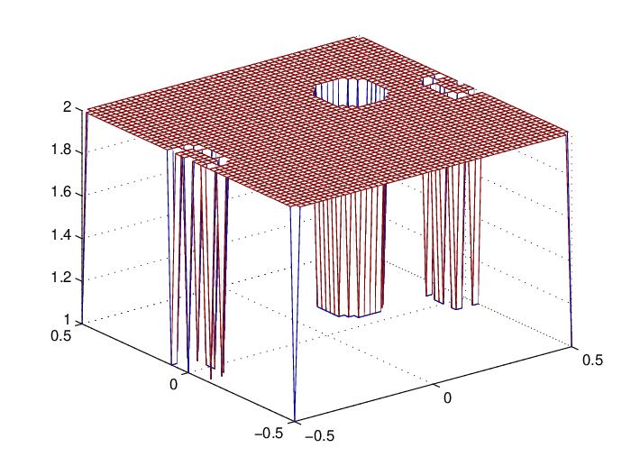
In Fig. 1(a), the red solid line and the blue dotted line coincide, that is to say, PCLSA can identify the shape of the air gap completely. In this test, the two functions, $\phi$ and $\phi_{exact}$, take the same value at every point $\textbf{\emph{x}}\in\Omega$. Fig. 1(b) shows the change of $F_{1}$ with respect to the number of iterations. From Fig. 1(b), we can see that the value of $F_{1}$ first becomes smaller, but doesn’t become smaller any more after 300 steps. So it is reasonable for us to choose $osci=10$. Fig. 1(c) to Fig. 1(f) show the evolution of the function $\phi$ and the interface. During the iterative process, the values of $\phi$ at the points of $\Omega$ develop towards to our expectation except four corner points. As the increase of the number of iterations, the values of $\phi$ at these four points first become small, which is away from our expectation, but becomes large after some steps. In Fig. 2, the values of the level set function $\phi$ at the four corner points and some points at the boundary of $\Omega$ are 1 instead of 2. By comparing with the picture of $\phi$ after 300 steps (see Fig. 1(f) and Fig. 2), we can see that it’s the effects of the regularization to let the values of $\phi$ at four points become large.

In this test, we set some variables as follows:

The initial guess of $\phi$ and the upper bound of $osci$ are chosen as $\phi_{0}=1.5$ and $15$, respectively. The iterative process stops after 212 iterations. We present the numerical results in Fig. 3.

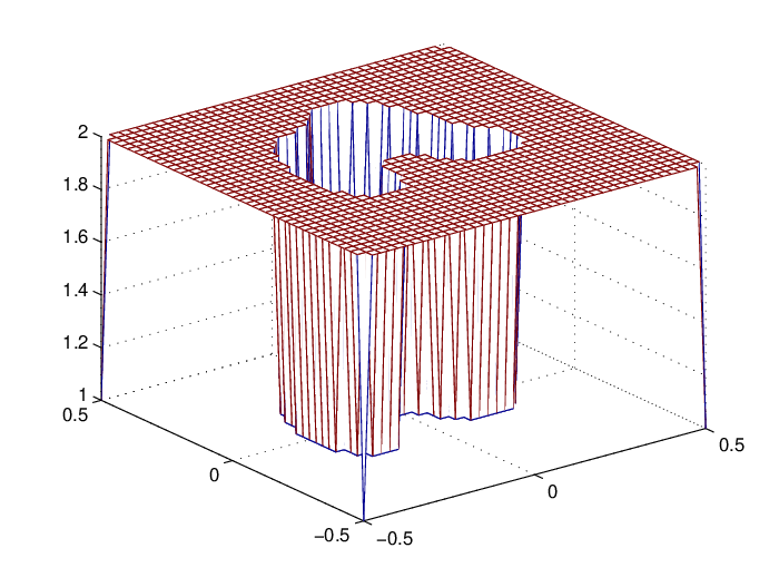
In Fig. 3(a), the red solid line coincides with the blue dotted one. And the number of the points where $\phi$ and $\phi_{exact}$ take different values is 0. That is, the algorithm can identify the shape of $D$ accurately. Fig. 3(b) depicts the change of $F_{1}$ with respect to the number of iterations. In Fig. 3(b), unlike Example 1, the value of $F_{1}$ is below $10^{-11}$ after some oscillations. Before exiting the iterative process, the times that the value of $F$ oscillates do not exceed 15, so it’s reasonable to choose the upper bound of $osci$ to be 15. Fig. 3(c) to Fig. 3(f) describe the evolution of $\phi$ and the interface. Similar to the evolution of the level set function $\phi$ in the Example 1, as the increase of the number of iterations, the values of $\phi$ at four corners first become smaller then start to increase to 2. In Fig. 4, the values of $\phi$ at four points of $\Omega$ are 1. Thus we can conclude that it is the effects of the regularization to pull the values of $\phi$ at these points back to 2.

In this test, the variables are chosen as follows:

The initial value of the level set function and the upper bound of $osci$ are $\phi_{0}=1.5$ and 10, separately. The iterative process stops after 306 steps. We present the numerical results in Fig. 5.

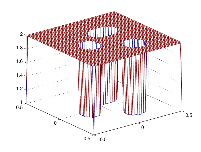
In Fig. 5(a), the interfaces between steel and air, represented by the red solid line and the blue dotted line, coincide. And the number of the points which $\phi$ and $\phi_{exact}$ take different values is 0. Fig. 5(b) depicts the change of $F_{1}$ with respect to the number of iterations. In Fig. 5(b), the value of $F_{1}$ first decreases and then oscillates in the last few steps. So it is reasonable for us to choose 10 as the upper bound of $osci$. Fig. 5(c) to Fig. 5(f) describe the evolution of $\phi$ and the interface. As the increase of the number of iterations, the values of $\phi$ at four corners first become smaller then start to increase to 2. In Fig. 6, the values of $\phi$ at four points of $\Omega$ are 1. Thus we can conclude that it is the effects of the regularization term to pull the values of $\phi$ at these points to 2.

Compared with the algorithm in [9], PCLSA takes much less steps, but reconstructs a more accurate shape. In [9], it takes 574 iteration steps to stop the algorithm. In our PCLSA, we only need half of that iterations, that is, totally 307 iterations to stop the algorithm. Moreover, with more iterations in [9] the final reconstruction shape still deviates a lot from the exact shape. In our final result (see Fig 5), however, there is no deviations at all. Thus PCLSA performs better than the algorithm in [9] for this example.

In order to show the flexibility of the initial guess of $\phi$, we assign different values to $\phi_{0}$ and compare the final results. we set $\phi_{0}$ to be different constants, that is, 1.2, 1.4, 1.7, 1.9, respectively, and present the final results in Fig. 7. For these four different values of $\phi_{0}$, the interfaces represented by $\phi$ and $\phi_{exact}$ coincide and the number of the points where $\phi$ and $\phi_{exact}$ take different value is 0. This indicates that our algorithm can identify the shape exactly. Furthermore, we choose a more general function as the initial value of $\phi$ and also observe the final interface. The general function is $\phi(x)=1+rand(x)$ where $rand(x)$ can produce pseudo-random values between 0 and 1. We present the numerical results in Fig. 8, where the interfaces represented by $\phi$ and $\phi_{exact}$ coincide.

From the above observation, PCLSA relies little on the initial value of the level set function. Thus, we need not to put too much attentions on the initial guess of $\phi$ in our PCLSA for the nonlinear electromagnetism recovery problems.

In this test, $dim=50$. We set $\phi_{0}=1.5$, the upper bound of $osci$ to be 10, $\alpha=0.1$ and $\sigma=0.9$. For different noise level cases, the final results are shown in Fig. 9. When the noise level is under 15%, the PCLSA reconstructs the shape of $D$ completely. That is, in our numerical test, the two functions $\phi$ and $\phi_{exact}$ take the same value at every point $\emph{\textbf{x}}\in\Omega$. But when the noise level is up to 20%, though the interface between the steel and air represented by $\phi$ is recovered, there are some flaws at the interface between $D$ and $\Omega\backslash D$ (some blue points). For the range of $\sigma$, the interval $0.6\sim 0.9$ is shown by our numerical tests to be not a bad choice.

However, $\sigma$ affects the iteration steps in our PCLSA. The larger $\sigma$ is, the less steps the algorithm takes. But at high noise level, the reconstructed shape is better when the value of $\sigma$ is smaller.

In this paper, we propose a piecewise constant level set algorithm for the nonlinear electromagnetism inverse problem. In our numeric test, our PCLSA do not rely on the initial guess of the level set function $\phi$, and can reconstruct the shape of $\Omega$ exactly even when the noise level is high. Our PCSLA is quite effective and robust to solve a kind of nonlinear inverse problems.

We express our gratitude to Doctor Ivan Cimrâk for his prompt and comprehensive answer to our problems. This work is supported by Natural Science Foundation of Zhejiang Province, China (No. LY12A01023), National Natural Science Foundation of China (No. 11201106) and Natural Science Foundation of Zhejiang Province, China (No. LQ12A01001).

References

- [1] S. Giguère, B. Lepine, J. Dubois, Pulsed eddy current technology: characterizing material loss with gap and lift-off variations, Research in Nondestructive Evaluation, 13 (2001), 119-129.
- [2] S. Osher, J.A. Sethian, Fronts propagating with curvature dependent speed: Algorithms based on Hamilton-Jacobi formulations, J. Comput. Phys, 79 (1988), 12-49.
- [3] S. Chen, B. Merriman, M. Kang, R.-E. Caflisch, C. Ratsch, L.-T Cheng, M. Gyure, R.-P. Fedkiw, C. Anderson, S. Osher, A Level Set Method for Thin Film Epitaxial Growth, J. Comput. Phys, 167 (2001), 475-500.
- [4] M. Burger, S. Osher, A Survey on Level Set Methods for Inverse Problems and Optimal Design, European J. Appl. Math, 16 (2005), 263-301.
- [5] L.A. Vese and T.F. Chan, A Multiphase Level Set Framework for Image Segmentation Using the Mumford and Shah Model, Int. J. Comput. Vis, 50 (2002), 271-293.
- [6] M.Y. Wang, X. Wang, D. Guo, A level set method for structural topology optimization, Comput. Methods Appl. Mech. Engrg, 192 (2003), 227-246.
- [7] N.M. Tanushev, L.A. Vese, A Piecewise-constant binary model for electrical impedance tomography, Inverse Probl. Imaging, 2 (2007), 423-435.
- [8] M. Sussman, P. Smereka and S. Osher, A level set approach for computing solutions to incompressible two-phase flow, J. Comput. Phys, 114 (1994), 146-159.
- [9] I. Cimrák, R. V. Keer, Level set method for the inverse elliptic problem in nonlinear electromagnetism, J. Comput. Phys, 229 (2010), 9269-9283.
- [10] I. Cimrák, Inverse thermal imaging inmaterials with nonlinear conductivity bymaterial and shape derivative method, Math. Methods Appl. Sci. 34(2011), 2303-2317.
- [11] I. Cimrák, Material and shape derivative method for quasi-linear elliptic systems with applications in inverse electromagnetic interface problems, SIAM J. Numer. Anal, 50 (2012), 1086-1110.
- [12] G. Allaire, F. Jouve, A.-M. Toader, A level-set method for shape optimization, C. R. Acad. Sci. Paris, Ser. I, 334 (2002), 1125-1130.
- [13] G. Allaire, F. Jouve, A.-M. Toader, Structural optimization using sensitivity analysis and a level-set method, J. Comput. Phys, 194 (2004), 363-393.
- [14] L. He, C.-Y. Kao, S. Osher, Incorporating topological derivatives into shape derivatives based level set methods, J. Comput. Phys, 225 (2007), 891-909.
- [15] G. Allaire, F. Jouve, A.-M. Toader, Structural optimization using topological and shape sensitivity via a level set method, Contr. Cybernet, 34 (2005), 59-80.
- [16] S. Amstutz, H. Andrae, A new algorithm for topology optimization using a level-set method, J. Comput. Phys, 216 (2006), 573-588.
- [17] M. Burger, B. Hackl, W. Ring, Incorporating topological derivatives into level set methods, J. Comput. Phys, 194 (2004), 344-362.
- [18] X. Wang, Y. Mei, M.Y. Wang, Incorporating topological derivatives into level set methods for structural topology optimization, in: T.L. et al. (Eds.), Optimal Shape Design and Modeling, Polish Academy of Sciences, Warsaw, 2004, 145-157.
- [19] X.C. Tai, T.F. Chan, A survey on multiple level set methods with applications for identifying piecewise constant functions, Int. J. Numer. Anas and Model, 1 (2004), 25-47
- [20] J. Lie, M. Lysaker and X.C. Tai, A variant of the level set method and applications to image segmentation, Math. Comp, 75 (2006), 1155-1174.
- [21] J. Lie, M. Lysaker and X.C. Tai, A binary level set model and some applications to Mumford-Shah image segmentation, IEEE Trans. Image Process, 15 (2006), 1171-1181.
- [22] J. Lie, M. Lysaker and X.C. Tai, Piecewise constant level set methods and image segmentation, in Scale Space and PDE Methods in Computer Vision, Lectures notes in Computer Sciences, 573-584.
- [23] J. Lie, M. Lysaker and X.C. Tai, A piecewise constant level set framework, Int. J. Numer. Anal. Model, 2 (2005), 422-438.
- [24] X.C. Tai, H.W. Li, A piecewise constant level set method for elliptic inverse problems, Appl. Numer. Math, 57 (2007), 686-696.
- [25] X.C. Tai, H.W. Li, Piecewise constant level set method for interface problems, Free boundary problems, Int. Ser. Numer. Math, 154 (2007), 307-316.
- [26] P. Wei; M. Y. Wang, Piecewise constant level set method for structural topology optimization. Internat. J. Numer. Methods Engrg, 78 (2009), 379-402
- [27] S.F Zhu, Q.B Wu, C.X. Liu, Variational piecewise constant level set methods for shape optimization of a two-density drum, J. Comput. Phys, 229 (2010), 5062-5089.
- [28] Z.F. Zhang , X.L. Cheng, A boundary piecewise constant level set method for boundary control of eigenvalue optimization problems, J. Comput. Phys, 230 (2011), 458-473.
- [29] J.L. Muller, S. Sitanen, Direct reconstruction of conductivities from boundary measurements, SIAM J. Sci. Comput, 24 (2003), 1232-1266.
- [30] D. Gilbarg, N.S. Trudinger, Elliptic Partial Differential Equations of Second Order, Die Grundlehren der Mathematischen Wissenschaften, Springer, 1977.
- [31] O.A. Ladyzhenskaya, N.N. Ural’tseva, Linear and Quasilinear Elliptic Equations, Mathematics in Science and Engineering, Academic press, 1968
- [32] S. Srinath, D.N. Mittal, An adjoint method for shape optimization in unsteady viscous flows, J. Comput. Phys, 229 (2010), 1994-2008.
- [33] H. Park, H. Shin, Shape identification for natural convection problems using the adjoint variable method, J. Comput. Phys, 186 (2003), 198-211.
- [34] S. Durand, I. Cimrâk, P. Sergeant, Adjoint variable method for time-harmonic Maxwell equations, COMPEL: Int. J. Comput. and Maths. in Electrical and Electric Eng, 28 (2009), 1202-1215.
- [35] P. Sergeant, I. Cimrâk, V. Melicher, L. Dupré, R. Van Keer, Adjoint variable method for the study of combined active and passive magnetic shielding, Math. Probl. Eng, (2008), 15pp.
- [36] I. Cimrâk, V. Melicher, Determination of precession and dissipation parameters in the micromagnetism, J. Comput. Appl. Math, 234 (2010), 2239-2249.
- [37] I. Cimrâk, V. Melicher, Sensitivity analysis framework for micromagnetism with application to optimal shape design of magnetic random access memories, Inverse Problems, 23 (2007), 563-588.