A global fit study on the new agegraphic dark energy model
Abstract
We perform a global fit study on the new agegraphic dark energy (NADE) model in a non-flat universe by using the MCMC method with the full CMB power spectra data from the WMAP 7-yr observations, the SNIa data from Union2.1 sample, BAO data from SDSS DR7 and WiggleZ Dark Energy Survey, and the latest measurements of from HST. We find that the value of is greater than at least at the 3 confidence levels (CLs), which implies that the NADE model distinctly favors an open universe. Besides, our results show that the value of the key parameter of NADE model, , at the 1–3 CLs, where its best-fit value is significantly smaller than those obtained in previous works. We find that the reason leading to such a change comes from the different SNIa samples used. Our further test indicates that there is a distinct tension between the Union2 sample of SNIa and other observations, and the tension will be relieved once the Union2 sample is replaced by the Union2.1 sample. So, the new constraint result of the NADE model obtained in this work is more reasonable than before.
pacs
95.36.+x, 98.80.Es, 98.80.-kI Introduction
Dark energy has become one of the most important research areas in cosmology since the cosmic acceleration was discovered by the observations of type Ia supernovae (SNIa) [1]. The cosmological constant, , introduced by Einstein in 1917, is a natural candidate for dark energy, which fits the observational data best to date. However, the model of plus cold dark matter, known as the CDM model, always suffers from the two well-known theoretical difficulties, namely, the fine-tuning and cosmic coincidence problems [2]. Thus, dynamical dark energy models become popular, because they may alleviate the theoretical challenges faced by the CDM model. For a recent review of dark energy, see Ref. [3].
Among the many dynamical dark energy models, a class with feature of quantum gravity, embodying holographic principle, looks very special and attractive. Such class of models, usually called “holographic dark energy”, has been investigated in detail [4] and constrained by the observational data [5]. In this paper, we focus on the “new agegraphic dark energy” (NADE) model [6] in this class, which takes into account the uncertainty relation of quantum mechanics together with the gravitational effect in general relativity. The reason that the NADE model is fairly attractive is also owing to the fact that this model has the same number of parameters to the CDM model, less than other dynamical dark energy models. The NADE model has been proven to fit the data well. However, it should be noticed that the global fit analysis on the NADE model has never been done.
The global fit analysis is very important for the study of a cosmological model. To determine the parameters of dark energy models, one often has them constrained by using some important observational data sets, such as SNIa, baryon acoustic oscillation (BAO) and cosmic microwave background (CMB). For the CMB information, to save time and power, one often uses the CMB “distance priors” (, , ) whose information is extracted from the temperature power spectrum of CMB based on a CDM scenario. However, it should be noted that using the CMB “distance priors” to constrain other dark energy models will lead to a circular problem, since the values of the CMB “distance priors” depend on a specific cosmological model, namely, the CDM model. Besides, the “distance priors” do not capture the information concerning the growth of structure probed by the late-time ISW effect which is sensitive to the properties of dark energy. In the past, the NADE model was constrained only by the CMB “distance priors” data. In this study, we shall use the full CMB data from the 7-yr WMAP observations to explore the parameter space of the cosmological model involving the NADE. Such an exploration is believed to complete the study of the NADE model.
In the previous studies, the spatial curvature, , is usually neglected. So, we do not know if a flat universe is still favored by current data in the NADE model. Moreover, the initial condition of the NADE model [6] is only applicable for a flat universe containing only dark energy and pressureless matter. In Ref. [7], a new, updated initial condition is proposed, which is applicable for a non-flat universe with various components. We shall apply this new initial condition in the present work. In such an application, for employing the “CosmoMC” package, one may treat the parameter as a derived parameter and use the Newton’s iteration algorithm to determine its value. In addition, in a global fit analysis, the cosmological perturbations of dark energy should also be considered. Thanks to the quintessence-like property of the NADE, there is no -crossing behavior and so the corresponding gravity instability is absent. In the holographic dark energy model, the -crossing happens, so one has to employ the parameterized post-Friedmann (PPF) approach to treat the gravity instability of the perturbations in a global fit analysis; for details see Ref. [8]. For the NADE model, however, we have no need to employ the PPF approach.
Our paper is organized as follows. In Sec. II, we derive the background and perturbation evolution equations for the NADE model in a non-flat universe. In Sec. III, we introduce the fit method and the observational data, and then give the global fit results. Concluding remarks are given in Sec. IV. In this work, we assume today’s scale factor , and so the redshift satisfies ; the subscript “0” always indicates the present value of the corresponding quantity, and the units with are used.
II Brief description of the NADE model
The NADE model is constructed in light of the Károlyházy relation and corresponding energy fluctuations of space-time. The energy density of NADE, , has the form [6]
| (1) |
where is a numerical parameter, is the reduced Planck mass, and is the conformal age of the universe,
| (2) |
where is the scale factor and is the Hubble parameter. Here a dot denotes the derivative with respect to the cosmic time .
The background evolution of a non-flat universe is described by the Friedmann equation,
| (3) |
where is defined as the ratio of the energy density to the critical energy density with , , , and which denotes the dark energy, dark matter, baryon, radiation and spatial curvature, respectively. Note that here .
The energy conservation equations for the various components take the form
| (4) |
where is the equation-of-state parameter (EOS) of a specific component denoted by subscript , such as , and . For the EOS of NADE, one can obtain
| (5) |
from Eqs. (1), (2) and (4). Furthermore, using Eqs. (1)–(4), one can also easily get the equation of motion of , a differential equation,
| (6) |
where with .
For solving the differential equation (6), we adopt the initial condition, at with , given in Ref. [7], which helps reduce one free parameter for the NADE model. This initial condition is an updated version of the original one, at , given in Ref. [9]. The only difference between them is that the new one is valid when the radiation is considered as a non-ignorable component. Note that the initial condition is also applicable in a non-flat universe, since the spatial curvature is much smaller than or at . For more details about the derivation and application of the new initial condition, see Ref. [7].
In our work, for simplicity, we fix according to the WMAP 7-yr observations [10], where is the standard value of the effective number of neutrino species and is the Hubble constant in units of 100 km/s/Mpc.
It should be noted that the parameters , , and are not independent. One of them can be derived from the others. For example, we can treat the parameter as the derived parameter. In this case, once the values of , and are given, one can impose an initial value of and then obtain the true value of by using the Newton iteration algorithm, , where with the th order numerical solution (at ) of Eq. (6) with the new initial condition, and is the numerical derivative of at the point . Of course, one can also treat or or as a derived parameter and get its value by using a similar method.
For our global fit analysis, it is convenient to modify the “CosmoMC” package [11] if is set as a derived parameter. Thus, we will use the Newton method mentioned above, which is proved to be convergent, to get the true value of . We choose the initial value and set a termination condition for the iteration, such as with a small quantity. Once Eq. (6) is solved, the Hubble expansion rate can be obtained by
| (7) |
With the background evolution of the NADE model completed, we now consider how to handle the perturbation of NADE. Since the EOS of NADE is always greater than , we can easily handle its perturbation. We take NADE as a perfect fluid with the EOS given by Eq. (5). In the synchronous gauge, the conservation of energy-momentum tensor gives the perturbation equations of density contrast and velocity divergence for the NADE in the Fourier space,
| (8) | |||||
| (9) |
Here , and are given by Eqs. (7) and (5). Other notation is consistent with the work of Ma and Bertschinger [12]. For the gauge ready formalism about the perturbation theory, see Ref. [13]. For the NADE, we assume the shear perturbation . In our calculations, the adiabatic initial conditions will be taken.
Finally, we feel that it may be necessary to make some additional comments on the treatment of dark energy perturbations in the NADE model. Actually, it is fairly difficult to calculate the cosmological perturbations of dark energy in the holographic-type dark energy models, because there is some non-local effect that makes the perturbation mechanism extremely obscure and hard to handle. This is the reason why for a long time no one addressed the issue of dark energy perturbations in a complete manner in the holographic-type models. Be that as it may, Li, Lin, and Wang [14] made a calculation for the perturbations in the holographic dark energy model, in which some approximations are used in dealing with the non-local integrals in the equations governing the evolution of metric perturbations, and they proved that the perturbations are stable for both super-horizon and sub-horizon scales. But a complete analysis of the cosmological perturbations in the holographic dark energy model is still absent. Thus, in the past, to avoid the inclusion of dark energy perturbation problem, one only used the CMB “distance priors” data, instead of the full CMB data, to constrain the holographic and agegraphic dark energy models.
However, recently, it was realized that, in order to make progress, one should first ignore the non-local effect in the holographic-type models and directly calculate dark energy perturbations in these models as if they are usual perfect fluids. Alone this line, global fit analyses on the holographic dark energy model were performed [8, 15]. It should be stressed, however, that such a treatment is only an expedient measure, in the case that we are not capable of completely handling the non-local effect in the calculation of dark energy perturbations in these models. But, on the other hand, since the non-local effect is not a dominant factor, it is believed that the fluid approximation in the holographic-type dark energy models is reasonable.
III Global fit results
In our global fit analysis, the parameter of the NADE model is treated as a derived parameter, whose value can be obtained by the parameters , and via the Newton iteration algorithm, as mentioned in Sec. II. The “CosmoMC” package uses the physical densities of baryon and cold dark matter instead of and . Thus, our most general parameter space vector is:
| (10) |
where is the ratio (multiplied by 100) of the sound horizon to the angular diameter distance at decoupling, is the optical depth to re-ionization, and are the amplitude and the spectral index of the primordial scalar perturbation power spectrum. For the pivot scale, we set Mpc-1 to be consistent with the WMAP team [10]. Note that we have assumed purely adiabatic initial conditions.
The sound speed of dark energy, , is usually treated as a phenomenological parameter for a fluid model of dark energy. It must be real and non-negative to avoid unphysical instabilities. In fact, if we treat the dark energy strictly as an adiabatic fluid, then the sound speed would be imaginary (in this case, the physical sound speed is equal to the adiabatic sound speed, ), leading to instabilities in dark energy. In order to fix this problem, it is necessary to assume that dark energy is a non-adiabatic fluid and impose by hand [16]. Our analysis is insensitive to the value of . As long as is close to 1, the dark energy does not cluster significantly on sub-Hubble scales. Therefore, in our analysis, we set to be 1; the adiabatic sound speed can be imaginary, . This is what is done in the CAMB and CMBFAST codes. Of course, one can also take as a parameter, but the fit results would not be affected by this treatment [17].
For the data, besides the CMB data (including the WMAP 7-yr temperature and polarization power spectra [10]), the main other astrophysical results that we shall use in this paper for the joint cosmological analysis are the following distance-scale indicators:
| Class | Parameter | Best fit with errors | ||
|---|---|---|---|---|
| Primary | ||||
| Derived | ||||
| (km/s/Mpc) | ||||
| Age (Gyr) | ||||


Our global fit results are summarized in Table 1 and Fig. 1. We notice two remarkable results: (i) the value of is greater than at least at the 3 confidence levels (CLs), which implies that the NADE model distinctly favors an open universe; (ii) the best-fit value of is evidently less than those obtained in the previous work.
The result of the spatial curvature we obtained is still at the level of , consistent with the other results about dark energy in the literature. However, it should be pointed out that our work is the first to show that the NADE model distinctly favors an open universe under current data.
The fit result of is at the 1–3 CLs. We find that the best-fit value of is significantly different from the results obtained in the previous work [7, 9, 22, 23, 25, 24]. For example, Refs. [7], [22], [24] and [25] gave , 2.807, 2.887, and 2.886, respectively. What can this change tell us? Next, we shall explore what the factor is that is making this change.
To do so, and without loss of generality, we take the most recent work in Ref. [7] as an example to make a comparison. We list here four different points between them: (1) the spatial curvature is considered in this work while it isn’t considered in Ref. [7]; (2) the Hubble constant measurement and the BAO measurement of parameter from the WiggleZ Dark Energy Survey are used in this work while they are not used in Ref. [7]; (3) the SNIa data set used in this work is Union2.1 sample while it is Union2 sample in Ref. [7]; (4) this paper performs a global fit where the full CMB information from WMAP-7yr observations is used while the CMB information used in Ref. [7] comes only from 7-yr WMAP “distance priors”. After testing these four items one by one by varying one condition and setting the others the same, we find that the change is mainly due to the different SNIa data used.
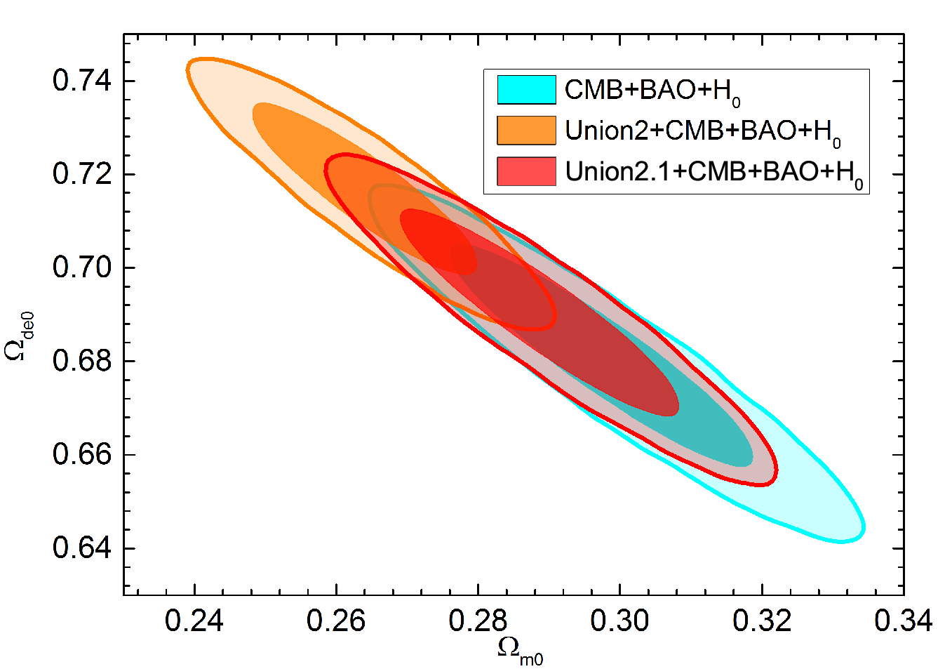
To see clearly, we plot the test results of different SNIa data used for the NADE model in Fig. 2. The cyan, orange and red regions denote the parameter spaces constrained by using the joint CMB, BAO and observations without SNIa data, with Union2 sample of SNIa data, and with Union2.1 sample of SNIa data, respectively. Note that the CMB data used here are the 7-yr WMAP “distance priors” for simplicity. Comparing the cyan region (without SNIa) with the orange region (with Union2), one can easily find that their overlapping region is very small, which implies that there is a tension between the Union2 sample of SNIa and the joint CMB, BAO and observations. However, the tension between SNIa and CMB+BAO+ will be greatly relieved once the Union2 sample is replaced by the Union2.1 sample of SNIa, since the overlap between cyan and red regions is very large. Thus, we can conclude that the new constraint result of the NADE model obtained in this work is more reasonable than before.
In addition, by using the global fit results obtained in this work (best-fit values), we plot the CMB power spectrum for the NADE model in Fig. 3. To make a comparison, we also plot the corresponding curve of the CDM model with the best-fit parameters given by the same data sets. The 7-yr WMAP observational data points with uncertainties are also marked in the figure. We can clearly see that the NADE model produces a different feature compared with the CDM model in the low regions. However, since the low data are rare and rough, the two models cannot be discriminated by the late-time ISW effects by far.
IV Concluding remarks
In this work, our main task is to perform a global fit analysis on the NADE model in a non-flat universe by using a MCMC method with the joint data of the full CMB spectra, BAO, SNIa and observations. We use the initial condition, at , to solve the differential equation of , which can reduce one free parameter for the NADE model. In order to easily modify the “CosmoMC” package, we set , , and as free parameters and as a derived parameter, and use the Newton iteration algorithm to obtain the true value of .
Our global fit results show that the NADE model distinctly favors an open universe, since the value of is greater than at the 3 CLs. Besides, we find that the value of the key parameter of the NADE model significantly different from those obtained in the previous work. We find that the main reason leading to such a change comes from the different SNIa samples used. Namely, the Union2.1 sample and the Union2 sample give fairly different constraint results for the NADE model. Our further test indicates that there is a distinct tension between the Union2 sample of SNIa and other observations, and the tension will be removed once the Union2 sample is replaced by the Union2.1 sample. Thus, we conclude that the new constraint result of the NADE model obtained in this paper is more reasonable than the previous ones.
We also plot the CMB power spectra for the NADE and CDM models by using the best-fit results of the global fits. It is shown that the NADE model and the CDM model produce slightly different features in the low regions. Since the low data are rather rare and rough, the two models cannot be discriminated by the late-time ISW effects yet. We expect that the future highly accurate data can do this job.
If dark energy is truly dynamical, as hinted by recent work [26], the possible non-gravitational interaction between dark energy and dark matter may deserve deeper investigations. In this work the interaction between dark energy and dark matter is not considered. If such an interaction exists in the NADE model, the calculations of the perturbations of dark energy and dark matter will become more complicated. The global fit analysis on the interacting agegraphic dark energy model is fairly attractive. In addition, the comparison of the various holographic models of dark energy under a uniform global fit is also necessary. We leave these subjects in the future work.
Acknowledgements.
This work was supported by the National Science Foundation of China under Grant Nos. 10705041, 10975032, 11047112 and 11175042, and by the National Ministry of Education of China under Grant Nos. NCET-09-0276, N100505001, N090305003, and N110405011.References
- [1] A. G. Riess et al. [Supernova Search Team Collaboration], Astron. J. 116, 1009 (1998); S. Perlmutter et al. [Supernova Cosmology Project Collaboration], Astrophys. J. 517, 565 (1999).
- [2] S. Weinberg, Rev. Mod. Phys. 61 (1989) 1; V. Sahni and A. A. Starobinsky, Int. J. Mod. Phys. D 9 (2000) 373; S. M. Carroll, Living Rev. Rel. 4 (2001) 1; T. Padmanabhan, Phys. Rept. 380 (2003) 235; P. J. E. Peebles and B. Ratra, Rev. Mod. Phys. 75 (2003) 559; E. J. Copeland, M. Sami and S. Tsujikawa, Int. J. Mod. Phys. D 15 (2006) 1753; J. Frieman, M. Turner and D. Huterer, Ann. Rev. Astron. Astrophys. 46, 385 (2008).
- [3] M. Li, X. D. Li, S. Wang and Y. Wang, Commun. Theor. Phys. 56, 525 (2011).
- [4] M. Li, Phys. Lett. B 603, 1 (2004); X. Zhang, Int. J. Mod. Phys. D 14, 1597 (2005); B. Chen, M. Li and Y. Wang, Nucl. Phys. B 774, 256 (2007); X. Zhang, Phys. Lett. B 648, 1 (2007); X. Zhang, Phys. Rev. D 74, 103505 (2006); C. Gao, F. Wu, X. Chen and Y. G. Shen, Phys. Rev. D 79, 043511 (2009); J. Zhang, X. Zhang and H. Liu, Eur. Phys. J. C 52, 693 (2007); X. Zhang, Phys. Lett. B 683, 81 (2010); M. Li and R. X. Miao, arXiv:1210.0966 [hep-th].
- [5] X. Zhang and F. Q. Wu, Phys. Rev. D 72, 043524 (2005); X. Zhang and F. Q. Wu, Phys. Rev. D 76, 023502 (2007); Q. G. Huang and Y. G. Gong, JCAP 0408, 006 (2004); Z. Chang, F. Q. Wu and X. Zhang, Phys. Lett. B 633, 14 (2006); J. Y. Shen, B. Wang, E. Abdalla and R. K. Su, Phys. Lett. B 609, 200 (2005); Z. L. Yi and T. J. Zhang, Mod. Phys. Lett. A 22, 41 (2007); X. Zhang, Phys. Rev. D 79, 103509 (2009); M. Li, X. D. Li, S. Wang, Y. Wang and X. Zhang, JCAP 0912 (2009) 014; Z. Zhang, S. Li, X. D. Li, X. Zhang and M. Li, JCAP 1206, 009 (2012).
- [6] H. Wei and R. G. Cai, Phys. Lett. B 660, 113 (2008).
- [7] Y. H. Li, J. F. Zhang and X. Zhang, Chin. Phys. B, in press, arXiv:1201.5446 [gr-qc].
- [8] S. Wang, Y. H. Li, X. D. Li and X. Zhang, arXiv:1207.6679 [astro-ph.CO].
- [9] H. Wei and R. G. Cai, Phys. Lett. B 663, 1 (2008).
- [10] E. Komatsu et al. [WMAP Collaboration], Astrophys. J. Suppl. 192, 18 (2011).
- [11] A. Lewis and S. Bridle, Phys. Rev. D 66, 103511 (2002).
- [12] C. P. Ma and E. Bertschinger, Astrophys. J. 455, 7 (1995).
- [13] J. c. Hwang and H. r. Noh, Phys. Rev. D 65, 023512 (2002).
- [14] M. Li, C. Lin and Y. Wang, JCAP 0805, 023 (2008).
- [15] L. Xu, Phys. Rev. D 85, 123505 (2012).
- [16] C. Gordon and W. Hu, Phys. Rev. D 70, 083003 (2004);J. Valiviita, E. Majerotto and R. Maartens, JCAP 0807, 020 (2008).
- [17] H. Li and J. Q. Xia, JCAP 1004, 026 (2010); H. Li and X. Zhang, Phys. Lett. B 713, 160 (2012)
- [18] N. Suzuki, D. Rubin and C. Lidman et al., Astrophys. J. 746, 85 (2012).
- [19] B. A. Reid et al. [SDSS Collaboration], Mon. Not. Roy. Astron. Soc. 401, 2148 (2010).
- [20] C. Blake, E. Kazin and F. Beutler et al., Mon. Not. Roy. Astron. Soc. 418, 1707 (2011).
- [21] A. G. Riess, L. Macri and S. Casertano et al., Astrophys. J. 730, 119 (2011).
- [22] M. Li, X. D. Li, S. Wang and X. Zhang, JCAP 0906, 036 (2009).
- [23] M. Li, X. Li and X. Zhang, Sci. China Phys. Mech. Astron. 53, 1631 (2010).
- [24] H. Wei, JCAP 1008, 020 (2010).
- [25] Y. Li, J. Ma, J. Cui, Z. Wang and X. Zhang, Sci. China Phys. Mech. Astron. 54, 1367 (2011).
- [26] G. B. Zhao, R. G. Crittenden, L. Pogosian and X. M. Zhang, Phys. Rev. Lett. 109, 171301 (2012); J. Z. Ma and X. Zhang, Phys. Lett. B 699, 233 (2011); H. Li and X. Zhang, Phys. Lett. B 703, 119 (2011); X. D. Li, S. Wang, Q. G. Huang, X. Zhang and M. Li, Sci. China Phys. Mech. Astron. 55, 1330 (2012).