A physical approach to the classification of indecomposable Virasoro representations from the blob algebra
Abstract
In the context of Conformal Field Theory (CFT), many results can be obtained from the representation theory of the Virasoro algebra. While the interest in Logarithmic CFTs has been growing recently, the Virasoro representations corresponding to these quantum field theories remain dauntingly complicated, thus hindering our understanding of various critical phenomena. We extend in this paper the construction of Read and Saleur [1, 2], and uncover a deep relationship between the Virasoro algebra and a finite-dimensional algebra characterizing the properties of two-dimensional statistical models, the so-called blob algebra (a proper extension of the Temperley–Lieb algebra). This allows us to explore vast classes of Virasoro representations (projective, tilting, generalized staggered modules, etc.), and to conjecture a classification of all possible indecomposable Virasoro modules (with, in particular, Jordan cells of arbitrary rank) that may appear in a consistent physical Logarithmic CFT where Virasoro is the maximal local chiral algebra. As by-products, we solve and analyze algebraically quantum-group symmetric XXZ spin chains and supersymmetric spin chains with extra spins at the boundary, together with the “mirror” spin chain introduced by Martin and Woodcock [3].
1 Introduction
While the subject of Logarithmic Conformal Field Theory (LCFT) appeared initially a little marginal, its importance has grown steadily over the last twenty years, following the pioneering papers [4, 5]. A LCFT is a two dimensional conformal field theory whose symmetry algebra – be it Virasoro, the product , a current algebra, SUSY extensions, etc. – exhibits reducible but indecomposable modules. It is not hard to see that this leads to logarithmic dependence of (some of) the correlation functions, as well as indecomposable operator product expansions.
Such unpleasant features are in fact unavoidable in many aspects of condensed matter physics. There, the unitarity of the CFT is not a requirement when one is interested in the description of geometrical, non local features in problems such as polymers or percolation (see e.g. [6] for a recent application); in the description of critical points in classical disordered systems, such as the random-bond Ising model; or in the description of some quantum critical points such as occur for non interacting electrons in a disordered potential in dimensions. Indecomposability also appears whenever one considers supergroup sigma models - such as the ones appearing on the string theory side of the AdS/CFT correspondence – or supersymmetric sigma models relevant to topological conformal field theory, as fully fledged quantum field theories, that is, beyond their “minimal” or “physical” sectors. Indecomposability is of course not restricted to two dimensions either, and it is believed to play a role in some four dimensional gauge theories as well [7].
With a little perspective, the interest in LCFTs is a very natural development in algebra, and naturally transposes to the quantum field theory context the extension of the theory of Lie algebras from the semi-simple to the non semi-simple case. As a result, the field of “non semi-simple CFTs” is currently witnessing a very fast expansion in mathematics [8].
Despite this growing interest, useful, tangible physical results are hard to come by. Very few LCFTs are fully solved for instance: apart from the ubiquitous symplectic fermions [9, 10], the list includes – and probably restricts to – the and WZW models, and the WZW model at level (see e.g. [11]). In particular, bulk four point functions in the case [12] remain sadly unavailable to this day.
One of the difficulties of LCFTs is the absence of methods to understand and control the amount of indecomposability one might expect to encounter in the general case. While models such as WZW theories on supergroups can be (partly) tackled because they admit semi-classical limits where intuition from supergeometry can be used, the world of, say, LCFTs at appears overwhelmingly hard to tame abstractly. This difficulty can in fact be given a clear mathematical formulation: for instance, it is known that the theory of representations of the Virasoro algebra is wild which means roughly that it is as complicated as can be [13, 14, 15]. Among the rather modest questions whose answer is not known is, for instance, the question of how large are the Jordan cells appearing in a given (chiral or non-chiral) CFT, such as the long searched for “CFT for percolation”.
As is often the case however, physics provides powerful constraints which can be used to restrict the wilderness of the algebraic problem. For instance, there is a large body of evidence that only a certain kind of modules appear in at least the simplest incarnations of supergroup WZW models, and this information can be put to very powerful use in concrete examples [16, 17]. Rather than getting into abstract considerations, it thus seems that important progress will be obtained by first studying in detail concrete models.
While supergroup WZW models can be tackled quite explicitly by using their semi-classical limit, the theories at that we expect to describe, say, percolation or the self avoiding walk problem do not offer such natural handles. In their case, it has turned out in fact to be most useful to have a closer look at lattice regularizations.
Lattice models indeed can be formulated in terms of associative lattice algebras such as the well known Temperley–Lieb algebra, which admits by now many generalizations, including the so called blob or one-boundary Temperley–Lieb algebra, the Birman–Wenzl–Murakami algebra, the Jones annular algebra, etc. The non-semi simplicity of the conformal field theoretic description of the continuum limit of the lattice models is prefigured naturally in the non semi-simplicity of these lattice algebras. A remarkable fact – first observed from characters identities many years back in some restricted cases [18] – is that the lattice algebras seem to exhibit, even in finite size, the exact same pattern of indecomposability as the continuum limit theory [2, 19]. While there are proposed mechanisms explaining this coincidence – in the simplest case, the common presence of an underlying “Lusztig” quantum group symmetry [20] – the fact is not entirely understood at the moment.
Nevertheless, a wealth of information has been obtained recently about indecomposable modules of the Virasoro algebra using this technique [21, 1, 2, 22], in agreement with results in abstract Virasoro representation theory [23, 24] of so-called staggered modules. The idea can be naturally extended to gain information about fusion [2, 25, 26, 19], and even to measure the logarithmic couplings [27, 28], whose value plays a key role in LCFTs. The extension to the case of and thus bulk logarithmic theories is an important but challenging direction – for recent progress here, see [29, 30, 31, 32].
The analysis in [1, 2] focussed mostly on lattice models with open boundary conditions, which are described algebraically in terms of the Temperley–Lieb algebra, and deeply related in the continuum limit to Virasoro algebra modules with lowest conformal weights (see eq. (21)), while a “dilute” version gives access to conformal weights . It is of utmost importance, in order to better understand all physically relevant indecomposable Virasoro modules, to generalize these ideas to conformal weights with both indices tunable at will. It was suggested in [21] that this should involve allowing for some extra degrees of freedom at the boundary, and in [33] that this idea corresponds, algebraically, to considering a one parameter extension of the TL algebra known as the blob or one-boundary Temperley–Lieb algebra.
The purpose of this paper is to study in details the correspondence between this algebra, the lattice models where it naturally plays a role, and the Virasoro algebra appearing in the continuum limit. While this looks like a rather technical endeavor, we believe that we are reaping a lot of rewards in the end, by obtaining what we believe (but do not prove) to be the first complete classification of Virasoro indecomposable modules possibly appearing in physical LCFTs where the Virasoro is the maximal local chiral algebra.
Obviously, this conjecture requires a careful definition of ‘physical’ LCFTs, this shall be discussed in details in Sec. 7. In a nutshell, we call physical LCFTs those conformal theories which are fixed points of interacting, non unitary, quantum field theories with well defined local actions11 1 The superprojective sigma models at topological angle are among possible examples of such non unitary theories.. Assuming that such physical LCFTs describing critical phenomena in percolation or self-avoiding walks do exist, we can expect that they must also admit some lattice regularizations involving local Hamiltonians and local degrees of freedom. Such lattice regularizations are typically quantum spin-chains with local interactions (susy spin-chains [34], XXZ models [2], etc). It is worth noting that in this context of local theories, the well known statistical loop models (see e.g. [33]) that are formulated using non local Boltzman weights, do not, in general, lead to physical field theories – it is known that their continuum limit does not coincide with any local field theory. Though the loop models can still be described using local field theories, they must be considered as some subsectors of these local field theories which we believe can be obtained as scaling limits of quantum spin-chains. Note that even though we define physical LCFTs as scaling limits of local quantum spin chains, thus excluding loop models, the latters can of course be thought of as interesting and physically-reasonable from the point of view of statistical mechanics. We will actually come back to loop models in this paper as the blob algebra provides new indecomposable modules for those theories too.

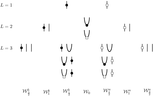
Our paper is written from the point of view of modules. Indeed, it is unclear for now whether there is a complete, general relation between the blob (an associative algebra) and the Virasoro (a Lie algebra) at an abstract level, but what we can do is to compare in details the structure of modules for the two algebras. The following discussion is thus split into two main parts. In the first one, we discuss the correspondence in the simplest case, by considering, on the Virasoro side, Verma modules, and on the blob side standard modules – together with their various types of submodules. An example of such correspondence is given at central charge in Fig. 1 (the notations for the blob algebra will be detailed in the following.) In the second part, we discuss the correspondence for a more general class of modules, in particular those that can appear in physical models, and whose structure is constrained, in particular by self-duality. These modules, called tilting, are different and more complicated than those considered in the first part, and their analysis requires some technical tools, which are discussed and summarized in a separate technical section. An example of such a module is provided in Fig. 2 where fields are simply represented by their conformal weight and the arrows increasing the conformal weight correspond to negative Virasoro modes while the arrows decreasing the weight represent the action of positive modes. We also note that such a “tilting” module contains Jordan cells of arbitrary rank, for example, there is a rank- Jordan cell in for the conformal weight , a rank- Jordan cell for the conformal weight and so on.

In more detail, our paper is organized as follows. Section 2 contains the basics: we review the blob algebra and its variants, some general aspects of its representation theory, how it appears in lattice models, and what it has to do with the Virasoro algebra. In section 3, we discuss the relationship between the blob and the Virasoro algebra at the level of well-known modules such as Verma modules. We demonstrate in particular a detailed correspondence – summarized in table 1 – between standard modules, quotients of standards and simple modules for the blob algebra on the one hand, and Verma, Kac and simple modules for the Virasoro algebra on the other hand.
While in the case of unitary conformal field theories, irreducible Virasoro (or some appropriate chiral algebra) modules are all that is needed, many kinds of more complicated, reducible but indecomposable modules, may appear in a LCFT. In fact, one of the purposes of the present analysis - and more generally of the associative algebraic approach to LCFTs - is to gain some general understanding of these modules. While the task is very difficult on the Virasoro side, it is much easier on the blob algebra side, thanks in part to mathematical theorems about so called cellular and other types of algebras studied recently in the mathematical literature [35]. In order to benefit from these results, the knowledge of a few definitions (such as projectiveness, self-duality, and tilting modules) is necessary. For convenience, we have gathered all such technical definitions in an algebraic reminder in section 4. We also describe the general structure of projective modules for the blob algebra in this section.
We are then able to study in section 5 the correspondence between the blob algebra modules appearing in the XXZ and supergroup boundary spin-chains on the one hand, and Virasoro staggered modules appearing in the continuum limit on the other. As a by-product, a large class of conformally invariant boundary conditions is introduced as the continuum limit of this family of boundary spin-chains.
Based on these examples and warm-ups, we take one step further in sections 6 and 7, which are arguably the main sections of this paper. In section 6, we discuss the “mirror” spin-chain first introduced in [3], which has the property of providing a faithful representation of the blob algebra. We analyze the corresponding Hilbert space decomposition in terms of tilting modules, which requires the use of mathematical concepts introduced in section 4. The continuum limit of these modules is then studied in section 7. In this last section, we provide a tentative classification of new families of indecomposable self-dual Virasoro modules, where in particular the Virasoro generator can have Jordan cells of arbitrary rank. We conjecture in fact that for a LCFT with Virasoro as the maximal local chiral algebra, all possible physical indecomposable modules should be obtained as the scaling limit of lattice tilting modules of the blob algebra or (sub)quotients thereof. This potentially tames22 2 Somehow in the same way the analysis of the semi-classical limit does for the WZW cases [36, 37]. the wilderness issue [13, 15].
Although the blob algebra plays a central role in our classification of physically relevant Virasoro modules, it also enters into the definition of non-local lattice models – such as boundary loop models [33] – that do not in general lead to physical field theories in the sense defined above. Even though we do not consider these loop models as proper lattice regularizations of physical LCFTs, they can obviously be considered as interesting in their own right, and relevant Virasoro modules in that context can also be described by the blob algebra. In section 7, we present a large family of indecomposable blob modules which can potentially describe boundary loop models. All these modules are realized in the continuum limit as non self-dual (in contrast to spin-chain modules) staggered Virasoro modules and their proper generalizations when three or more Verma modules are glued with each other. A few conclusions are gathered in section 8. Finally, three appendices contain rather technical and supplementary material.
Notations
For convenience, we collect here some notations that we shall use throughout this paper:
- •
: Temperley-Lieb algebra on sites with loop fugacity ,
- •
: blob algebra on sites, with fugacity for boundary loops,
- •
: Standard modules over the blob algebra corresponding to through lines in the blobbed () or unblobbed () sector,
- •
: the JS blob algebra (see section 2.2),
- •
: Standard modules over (see section 2.2),
- •
: Verma modules over the Virasoro algebra with conformal weight ,
- •
: Verma modules with the weight where and are the Kac labels,
- •
: quotients of standard modules over the blob algebra (see section 3.1),
- •
: Kac modules – quotients of Verma modules over the Virasoro algebra (see section 3.1),
- •
and : Jones-Wenzl projectors (see eq. (34)),
- •
: the “quotient” blob algebra (see section 3.1).
- •
: Simple modules over the blob algebra,
- •
: Projective modules over the blob algebra,
- •
: Tilting modules over the blob algebra (used in section 6),
- •
: Quantum group -deformation of SU,
- •
: Standard (Weyl) modules of ,
- •
: Simple modules over ,
- •
: Tilting modules over ,
- •
: Staggered modules over the Virasoro algebra.
Before starting, we emphasize that, while this paper deals with rather mathematical concepts, its style and emphasis are definitely non rigorous, though the analysis on the lattice part is rather formal and mathematically precise. More rigorous work in the same spirit can be found in [29, 30, 31]. Note also that our analysis uses extensively the thorough numerical conjectures of [33] and the algebraic results of [38].
2 Preliminaries
In this section, we define the blob algebra and its generic representation theory. We motivate the introduction of this algebra by discussing boundary conditions in loop models and we discuss how a slightly deformed version of the blob algebra, that we shall call “JS blob algebra”, is in fact more natural from a physical point of view [33]. We will also introduce some notations that we will use throughout this paper.
2.1 The blob algebra and its standard modules
blob algebra.
In this paper, we shall study models based on the blob algebra, also called one-boundary Temperley-Lieb algebra . This algebra – which now plays an important role in the study of affine Hecke algebras [39], and admits various generalizations as well [40] – seems to have been introduced first in the mathematical physics literature in [41]. It is a two parameters algebra, conveniently defined using decorated Temperley Lieb diagrams. We will assume in the following that the reader is familiar with the Temperley-Lieb algebra (see [42] for a recent review), its representation theory when is generic and its interpretation as an algebra of diagrams. To define the blob algebra, consider now () strands and all the words written with the generators () and an extra generator , subject to the relations
| (1a) | |||||
| (1b) | |||||
| (1c) | |||||
| (1d) | |||||
| (1e) | |||||
| (1f) | |||||
This algebra is of course nothing but the usual Temperley-Lieb algebra with an extra boundary operator , which decorates lines with a “blob”, and gives to blobbed loops a different weight [41].
We also define and with , and parametrize the weights as
| (2) |
and
| (3) |
where is a real number and we use the -numbers
| (4) |
In the notations of Martin and Woodcock [38] (a reference we will use frequently in what follows), , and . We can also introduce so that with . We restrict ourselves to the case , as negative ’s are simply related to the case by a switch between and . Note also that we see from eq. (3) that one can choose to be in what we shall call the “fundamental domain” .
The operators and are best understood diagrammatically. Introducing the notation
and
the equations (1) can now be interpreted geometrically. The composition law then corresponds to stacking the diagrams, where it is assumed that every closed loop carries a weight , while closed loops carrying a blob symbol (or more) get a different weight . Within this geometrical setup, the algebra itself can be thought of as an algebra of diagrams.
Generically irreducible representations.
The blob algebra has the important property [35] of being “cellular”, which roughly means, that when considered as an algebra of diagrams, the states can be cut in half, forming “reduced states” in the physicist language of the transfer matrix. These reduced states may be used as a basis to construct the so-called “cell” or standard modules of the algebra, which are in fact the irreducible representations for generic (non integer).
The standard modules for the blob algebra are well known and can be easily constructed geometrically. They are parametrized by the number of through lines propagating through the system, i.e., extending from the bottom to the top in the diagrammatic representation. Within a standard module, through lines cannot be contracted by the TL generators . In addition, the standard modules carry a label ( or ) whose meaning we now explain. We introduce an “unblob” or “antiblob” operator , which is an idempotent just like itself. It is represented by a symbol ‘’ instead of ‘’. Moreover, the blob operator and the unblob operator are orthogonal projectors. When there are through lines in the system (), only the leftmost line is exposed to the boundary where and act. We can choose a basis so that the leftmost through line is either blobbed by the symbol ‘’ or unblobbed, with symbol ‘’, and it has to stay that way under the action of the transfer matrix or spin-chain hamiltonian (see below). We then denote the standard module with no through lines, and (resp. ) the standard module with through lines in the blobbed (resp., unblobbed) sector.
Following Ref. [41], the standard modules can be constructed iteratively using a Pascal triangle construction (see Fig. 3). The action of the algebra on states can be obtained geometrically by stacking the diagrams on top of one another, just as for the Temperley-Lieb algebra with the convention that the TL generators cannot contract two through lines. This convention implies that each standard module is stable under the action of the algebra. The blobbed and unblobbed standard modules have the same dimension
| (5) |
Indeed, the Pascal construction of the state is compatible with the standard recursion relation . The dimension of is therefore
| (6) |
These standard modules are irreducible for any and when is not an integer (generic). Finally note that throughout all this paper, we shall mostly restrict to the case integer, so that is even and is integer. In any case has the same parity as .
Scalar product.
We also mention the existence of a natural symmetric bilinear form for the blob algebra, that we will loosely call scalar product. In a given standard module, the scalar product of two basis states and , denoted , is defined geometrically by taking the mirror image of by a horizontal reflection, and gluing it on top of . If a pair of through lines is contracted in the process, we define the scalar product to be , otherwise, its value is simply given by the weights of the loops in the resulting diagram. Let us illustrate this with a few examples
| (7a) | |||||
| (7b) | |||||
| (7c) | |||||
An important point is that the generators of the blob algebra are self-adjoint for this scalar product, that is, and .
2.2 The JS blob algebra and its standard modules
The JS algebra
For reasons that will become clear later, it will be useful for us to consider a smaller algebra, that we will call the JS blob algebra [33, 43], obtained via
| (8) |
Note that by this definition, any element of the JS algebra is an element of sandwiched between two ’s. In terms of diagrams, the action of the generators of guarantees that every loop touching the left boundary carries a blob symbol.
A crucial observation is that when , this algebra is isomorphic to another blob algebra on a smaller number of sites and with different parameters. More explicitly, we have an isomorphism of associative algebras
| (9) |
The proof of this statement is elementary, denoting and , for , the generators of , one can readily check that the identity in the JS algebra is and the generators
| (10) |
satisfy all the relations of the blob algebra .
In the particular case , the element from (10) is not defined. Introducing then and , the algebra is then isomorphic to yet another variant of the blob algebra generated by , with , and with the relations (1) except the two last ones which read now
| (11) |
Notice that, since , there is no possible isomorphism of this algebra with a blob algebra. Representation theory in this case is more peculiar and will be discussed separately below in this section and in Sec. 3.2.2 and 4.1.
Standard modules over the JS algebra
The standard modules over the JS blob algebra are readily obtained from those of the original blob algebra by acting with , i.e., they are images of under its action in . We will use a hat to denote the representations of (e.g. ).
Recalling the isomorphism (9) and (10) of associative algebras, the correspondence with the standard modules over is the following. We find that the JS blobbed modules labeled with are unblobbed standard modules with through lines for , and that JS unblobbed modules with through lines are blobbed standard modules with through lines. In other words, we have the isomorphisms and , with a positive integer not exceeding (note that ), and where modules in the right-hand side of these equations are over . The rigorous proof of this statement is rather technical so we shall not go into these formal details here. We note that the module with no through lines should be considered as unblobbed [43] and hence . Note also that using the dimensions of the standard modules for , we immediately find the dimensions of the JS standard modules
| (12a) | |||||
| (12b) | |||||
These dimensions can also be obtained using combinatorics [43].
In the case of non-zero , we will use the algebra isomorphism to study the representation theory of using the results of [38]. The case requires more work because it is not covered in [38]33 3 Note however that this case is part of the results in [39] that uses the representation theory of the affine TL algebra along with the so-called braid translator. We follow here a more direct route.. In the case , we find that the two non isomorphic modules and over the blob algebra become isomorphic for the JS blob algebra:
| (13) |
To show this, let us introduce the linear map , whose action on the basis states of is given by
| 0,0)(9,2) psellipticarc[linecolor=black](7,0.5)(0.5,0.35)180360 |
where we have represented only the first three leftmost through lines of the state in . In simple words, joins the first two leftmost through lines of the state in , and puts an antiblob symbol on the third one if the latter exists. The resulting state belongs to indeed, with the convention . It is straightforward to check that this is a one to one mapping so that is an isomorphism between vector spaces. Moreover, when , is an intertwining operator of . The main point in this last claim is that 0,0)(1.5,1) psellipticarc[linecolor=black,linewidth=1.0pt]-(0.5,1.0)(0.5,1.42)180360 behaves exactly like two through lines when , in particular, it is annihilated by the corresponding Temperley-Lieb generator 0,0)(1,1) psellipticarc[linecolor=black,linewidth=1.0pt]-(0.5,1)(0.355,0.355)180360 psellipticarc[linecolor=black,linewidth=1.0pt]-(0.5,0)(0.355,0.355)0180 . The representations and are therefore equivalent when the weight of the blobbed loops vanishes . We will denote this representation for the JS algebra as , without the superscript
| (14) |
The isomorphisms (13) will turn out to be important in what follows44 4 Note that such isomorphisms can be checked numerically, at least for generic when the modules are simple. In particular, we found that the transfer matrix (see below) has exactly the same spectrum in the modules and , etc..
2.3 The blob algebra in statistical mechanics models
Transfer matrix and loop models
We will study models defined by their transfer matrix
| (15) |
or by the -dimensional quantum hamiltonian
| (16) |
The transfer matrix acting on standard modules should be thought of in terms of a geometrical loop model. Let us represent its action in terms of plaquettes
| 0,0)(9,2.25) psellipticarc[linecolor=blue](7.5,1.5)(0.53033,0.53033)31545 |
where in this example (). The rightmost half plaquette corresponds to a free boundary condition whereas the first half plaquette may or may not carry a blob symbol. The bulk plaquettes carry the usual action of the Temperley-Lieb generators
| 0,0)(10,2) psellipticarc[linecolor=blue](5.25,1)(0.53033,0.53033)31545 psellipticarc[linecolor=blue](6.75,1)(0.53033,0.53033)135225 psellipticarc[linecolor=blue](9,0.25)(0.53033,0.53033)45135 psellipticarc[linecolor=blue](9,1.75)(0.53033,0.53033)225315 |
whilst the first one represents
| 0,0)(10,2) psellipticarc[linecolor=blue](6.75,1)(0.53033,0.53033)135225 psellipticarc[linecolor=blue](9.75,1)(0.53033,0.53033)135225 |
The action of this transfer matrix builds up loop configurations, where the edges touching the boundary may or may not be blobbed, depending on the parameter . In addition to these factors, the Boltzmann weight of a configuration is computed by attributing a weight to closed loops carrying at least one blob symbol, and a weight to the other loops. The blob algebra is completely symmetric between blob and antiblob operators, and it is convenient to introduce the diagrammatic representation
| 0,0)(4,2) psellipticarc[linecolor=blue](3.75,1)(0.53033,0.53033)135225 |
where the box represents the antiblob operator, and each loop carrying at least one box will be weighted by . Note also that configurations with at least one loop that is blobbed and unblobbed at the same time should be excluded from the partition function, since .

Thanks to the extensive numerical study of [33] and the Bethe ansatz results of [44, 45], the phase diagram of this statistical model in terms of the boundary coupling is now well understood, and can be summarized by the diagram below:
| 0,0)(9,2) |
Here, the fixed point corresponds to free boundary conditions, and is described algebraically by the Temperley-Lieb algebra. The perturbation by the boundary coupling is relevant in the renormalization group sense, so that the system flows to one of the two conformally invariant boundary conditions where every loop touching the left boundary carries a blob or unblob symbol. These two fixed points are related by a simple switch between the weights of blobbed and unblobbed loops, and in the following we will focus only on the fixed point .
The limit in the transfer matrix , corresponds to blobbing every loop touching the boundary; the transfer matrix reads then schematically
| 0,0)(9,2.25) psellipticarc[linecolor=blue](3,1.5)(0.53033,0.53033)135225 psellipticarc[linecolor=blue](7.5,1.5)(0.53033,0.53033)31545 |
and an example of loop configuration in this case is shown in Fig. 4. The limit has the advantage of reducing the dimension of the Hilbert space while keeping the correct universality class in the continuum limit: the relevant algebra indeed is now the JS blob algebra . In addition of being more pleasant physically and more convenient numerically, we will show in the following that this limit leads also to the correct algebraic object to consider for studying the correspondence with the Virasoro algebra.
2.4 Connections with the Virasoro algebra
The scaling limit
At the renormalization group fixed point , we expect statistical mechanics systems with transfer matrix (15) to exhibit conformal invariance at low energy, and their scaling limit to be described by a conformal field theory.
In agreement with the renormalization group flow described previously, one finds (numerically as well as analytically [33, 44, 45]) that the low energy properties are indeed independent of the parameter (or in the Hamiltonian point of view). The central charge can be extracted from the scaling of the ground state eigenvalue [46], and it takes the well known form
| (17) |
where we recall that parametrizes the loop weight .
The subdominant eigenvalues are related to the conformal dimension (critical exponent) of the operators in the underlying boundary conformal field theory
| (18) |
Which exponents are obtained, and with which multiplicity, depends on the sector of the transfer matrix, and the particular representation of the blob algebra one considers: so far, we have implicitly assumed that we were dealing with a loop model, but in fact many other representations are possible, and relevant physically as well as formally.
Restricting for now to loop models, one can compute the low-energy spectrum in the scaling limit and identify all the exponents occurring in the spectrum of the transfer matrix (or the hamiltonian) acting in the standard modules over the blob algebra. It is convenient to gather the results into a generating function (character) , where the sum is taken over all low-energy states. In the sector with no through lines, one finds [33]
| (19) |
with
| (20) |
and
| (21) |
On the other hand, the generating functions [33] for the blobbed and unblobbed sectors read
| (22a) | |||||
| (22b) | |||||
Some important points are worth mentioning before going further:
- •
In all these formulas involving critical exponents, we have . In particular, we have to keep in mind that is defined modulo . However, the correspondence (22) with the conformal exponents is obviously only correct in the fundamental domain . Recall nevertheless the symmetry of the conformal weights: , for any real numbers and . Using this symmetry we actually cover the full extended Kac table, when .
- •
Algebraically, there is a symmetry between the blobbed and unblobbed sectors – realized, in practice, by swapping the loop weights and while switching the modules and . This is because of the symmetric role of the operators and in the definition of the blob algebra. This symmetry is however broken by the choice of the transfer matrix, and the critical exponents do depend on the sign of the coupling, which we chose to be here. To illustrate this point, consider a simple example with . For ( and ) and in the blobbed sector, we find a critical exponent . For ( and ) and still , we find in the unblobbed sector a completely different exponent . Therefore, unblobbed and blobbed exponents are not switched when swapping the blobbed and unblobbed loop weights.
We comment finally on the spectrum of the standard modules over the JS blob algebra. It was argued in [33] that, in agreement with the renormalization group flow, the full spectrum of critical exponents obtained for was the same as for . This can also be checked directly using our formulas (22a) and (22b) for the critical exponents. We first note that the change in the isomorphism corresponds to the change of the Kac label . Using the isomorphism of the standard modules, for , one finds that the critical exponent corresponding to reads
as it is expected. An analogous argument shows that the critical exponent corresponding to is indeed as expected.
For the case , the critical exponent corresponding to is . Note that we have an identity compatible with the isomorphism (14). The case will be discussed in more detail below.
Standard versus Verma modules
Consider now the fully generic case, where is not a root of unity and is non integer. In this case, the standard modules are irreducible, and the central charge of the corresponding CFT is also generic. It is then interesting to observe that the generating function
| (23) |
coincides with the character of the Verma module , which is also irreducible when and are generic. Recall [47] that a Virasoro Verma module is simply defined by letting the lowering part of the Virasoro algebra to act freely on a highest weight state . The character of the Verma module is then given by the right-hand side of eq. (23) when .
We thus observe an intriguing connection between two a priori quite different objects: standard modules for an associative algebra, and Verma modules for an (infinite dimensional) Lie algebra. Similar connections have been observed in other contexts. Their physical origin is that one presumably can, in the scaling limit, build expressions in terms of the lattice generators whose action, on a properly chosen subset of states (the scaling states) provides a representation of the Virasoro algebra. Except in very favorable (free of interactions) cases [48, 49, 31] however, such a construction has never been fully completed. We will give below a sketch of how this might go for the blob algebra. Note also that non isomorphic standard modules over the blob algebra with a fixed value of give rise to non isomorphic Verma modules in the scaling limit55 5 Indeed, recalling the isomorphism of the Verma modules and , i.e., for those having the same conformal weight , see eq. (21), we note that these Verma modules can be obtained from different standard modules and , with . However, these are over different blob algebras defined by different -parameters and , respectively, and defined for different parities of the total number of sites (one should fix the parity of the number of sites before taking the limit). .
It is tempting and fruitful however to remain at a more global level, and wonder whether the relationship between standard and Verma modules in the generic case carries over to degenerate cases. Of course, the correspondence between the generating functions for standard modules and the characters of Verma modules holds for non-generic values of , or integer , as well. On the Virasoro side, it is well known that in these cases the Verma modules become reducible, and exhibit a more or less intricate structure of sub-modules. The same is true for the blob algebra. The decomposition of Verma/standard modules can be summarized by some simple data: the set of simple (irreducible) sub-modules, together with arrows indicating maps by elements of the algebra. The key question is then, does the connection between the two algebras still hold at this more detailed level? This is the point we shall address in the next section.
From the JS algebra to Virasoro generators
The relationship between central charge and critical exponents on the one hand, and the scaling of the transfer matrix (Hamiltonian) eigenvalues corresponds formally to the fact that the Hamiltonian behaves like
| (24) |
where is the Fermi velocity [18], and are non-universal quantities, and is the usual Virasoro zero mode. We recall that and , with .
A little more precisely, the scaling limit is obtained by considering a finite number of low-energy eigenvectors of the Hamiltonian, computing the matrix elements of the desired operators between these scaling states in the limit of large size , and then taking the limit . This double limit procedure is necessary to obtain a quantum field theory describing the low-energy physics of a given lattice system. In particular, we expect a certain combination of the local Hamiltonian densities to reproduce in the scaling limit, on this basis of low-energy scaling states, the action of the Virasoro generators . This was discussed in the context of the TL algebra in Ref. [49], following the pioneering work of Kadanoff and Ceva [48].
In our example of the Hamiltonian , it is rather easy to come up with a conjecture for the expression of Virasoro generators on the lattice. Recall first that one can choose safely any while remaining in the same universality class. Second, using the isomorphism (9) between the JS blob algebra and another blob algebra, one can rewrite the Hamiltonian as , defined on sites up to a switch . In fact, since we have seen that the JS version of the blob algebra is the physically more correct object to consider, we will work with as our fundamental Hamiltonian defined on sites, acting on a Hilbert space where all states are in the image of the operator so that .
Actually, when acting on we only need one factor of in the expression of the Hamiltonian, so that the “blobbed” Hamiltonian is simply related to the usual TL Hamiltonian by . This is because any state satisfy . Meanwhile, the factor in ensures that the image of is indeed in . In the continuum limit, we expect the Hamiltonian to tend, up to a scaling factor, to the Virasoro generator . Therefore, we expect the following lattice regularization for this generator . To obtain a lattice version of the other Virasoro generators , following [49], it is useful to think in terms of an anisotropic version of our lattice model
| (25) |
where
| (26) |
Here, parametrizes the anisotropy (spectral parameter) and . An important point is that the derivation of the lattice generators in [49] relies only on a definition of the stress energy tensor in terms of the straining of the lattice (we refer the reader to [49] for more details), which is a bulk property that we do not expect to be modified by the blob operator . This means that the lattice expression of the Virasoro generators in the blob case should take the same form as in [49], only with an additional multiplicative factor.
We thus conjecture that the Virasoro generators on the lattice in terms of the elements of take the form66 6 It is worth pointing out that all the operators in this expression belong to the JS blob algebra . However, the factors on the right are not strictly necessary since the Hilbert space we are working with satisfies , so we might as well use instead of .
| (27) |
where is the groundstate energy density for . Using Bethe ansatz methods, one can show [50] that
| (28) |
The operators are expected to tend to the Virasoro modes in the double limit sense explained above, that is, their matrix elements between scaling (low-energy) states should converge to Virasoro operators. In the case , this lattice regularization of the Virasoro algebra proved very useful to measure numerically Virasoro matrix elements in [49], and in particular, it was used extensively to determine the so-called indecomposability parameters in the context of logarithmic CFTs [28]. We leave the verification of this formula in other cases for future work.
3 From the representation theory of the (JS) blob algebra to Virasoro
We now wish to study what happens to the similarities between the standard modules over the (JS) blob algebra and the Virasoro Verma modules in degenerate cases. To make a long story short, we will see that everything keeps working quite beautifully. Only in the case will there be a small subtlety related to the distinction between what we called JS blob algebra and the blob algebra, and we shall show that only the JS version completely matches the known results of Virasoro representation theory. The main results of this section are gathered in Tab. 1.
3.1 Singly critical cases and Kac modules
Let us turn to a slightly more involved case which is usually referred to as “singly critical” for the blob algebra representation theory [38]. Keeping generic, let us recall the parametrization (3) of the blob parameter and consider the case integer, for which the standard modules are in general not irreducible anymore. Then for positive77 7 The case negative is obviously obtained by switching the blob and unblobbed labels everywhere. , it is well known [41] that one has the following injective homomorphisms (embeddings)
| (29a) | |||||
| (29b) | |||||
The other standard modules with remain irreducible. Because of these embeddings, we can define the quotients , and similarly for , which are irreducible as long as remains generic. We shall refer to these modules as “quotient” modules over the blob algebra.
These quotient representations and have dimensions
| (30a) | |||||
| (30b) | |||||
and their generating functions of scaling states are given by the Virasoro characters
| (31a) | |||
| (31b) | |||
The crucial observation is that the corresponding Verma module becomes also reducible when is integer, and has a proper submodule at level isomorphic to which is precisely the Verma module associated with . We represent the structure of this Verma module by the diagram
| (32) |
where the arrow represents the action of , of ’s with here, and we denote irreducible subquotients by the corresponding conformal weights. The quotient is called a Kac module88 8 We note that there exist several inequivalent definitions of Kac modules in the literature. One of them uses quotients of Verma modules, the convention chosen here, and another uses quotients (and submodules) of Feigin–Fuchs modules, see e.g. [51]. and we denote it by . This module is irreducible when the central charge is generic. Its character
| (33) |
corresponds exactly to the generating functions (31).
An explicit construction of these quotient modules in a basis was given in [38] and [33] (see also [52, 53]). Following [33], they can be described in terms of “ghost” strings added to the left of the usual Temperley Lieb standard modules with through lines. Using the so-called -symmetrizer operator [33] (closely related to the Jones-Wenzl projectors that we will introduce in the next paragraph) and the usual TL generators, it is possible to define representations that coincide with these quotients. We remark that this construction is related to the integrable boundary conditions of Ref. [21], that uses similar projectors, although the models there correspond rather to a fusion of blob modules that we shall not discuss here.
The quotient blob algebra
To be more precise, it is also useful to define a quotient of the blob algebra that will have the quotient modules as standard (cell) modules. We follow here Ref. [38], and introduce a generalization of the Jones-Wenzl projectors to the blob algebra, that is, we construct projectors on the unblobbed sector with number of through lines , defined recursively by
| (34a) | |||||
| (34b) | |||||
We then introduce the quotient (only for positive integer) algebra99 9 Note that for , we could introduce similar projectors onto blobbed sectors with number of through lines .
| (35) |
which is nothing but the blob algebra where the ideal spanned by the projector has been quotiented out. We shall call this algebra the quotient blob algebra, and we will see that the representation theory of this algebra is simpler than that of . In particular, the projective modules (see next section for some reminders on this important concept) over can be at worse of diamond shape whereas projective covers for are much more complicated.
Taking the quotient (35) by the two-sided ideal generated by means that we remove all modules (and subquotients) isomorphic to . Then note that is isomorphic to the Temperley–Lieb algebra , as can be readily shown ( in this case) by setting to zero all the diagrams that contain the antiblob symbol. The quotient blob algebra is still a cellular algebra and its standard modules are given precisely by (and , for … ). In particular, one can show using the RSOS picture that the projector acts as in the ghost string representation [53] (for a definition of RSOS models, see e.g. [54]).
3.2 Doubly critical cases: blob algebra representation theory at and
Finally, we turn to the most interesting case, with root of unity or integer (which is necessary to describe most of the physically relevant examples), and integer in the fundamental domain , so the rational conformal weights lie within the (extended) Kac table. The representation theory of the blob algebra is much richer is this case. For simplicity, we shall focus on the example of boundary Percolation (, ). The generalization to other roots of unity is straightforward. In this section, we will follow closely [38]1010 10 Note that when is integer, the parameter is defined modulo . In order to be consistent with [38], we fix its value as , see section 7 in [38]..
3.2.1 Case
0,0)(10,2)
0,0)(10,3)
The structure of the standard modules of is described in [38], we will work them out explicitly here. Let us begin with the case which corresponds to giving the weight to blobbed loops. We shall see that everything goes over smoothly to Virasoro here, but the situation will be more intricate later.
The case may seem trivial as it seems to reduce to the ordinary Temperley–Lieb case. However, one must remember that the blob algebra is in fact bigger, and reduces to the TL algebra only after taking a quotient by the ideal generated by the Jones–Wenzl projector . The structure of the standard modules can be obtained from a weight diagram [38], similar to those encountered in Lie algebra theory. The weight diagram in Fig. 5 is constructed with walls at , and we call the fundamental alcove the domain containing the origin. There is a correspondence between the integers on the weight diagram and the standard modules as is the number of through lines in the blobbed (resp., unblobbed) sector if (resp., ). The structure of the standard modules in the fundamental alcove is given by reflexions through the walls which lie outside the interval defined by the weight and the origin (see [38]). These (allowable) reflections correspond to embeddings of the standard modules. To see how reflection works, let us work out a simple example of structure. Using Fig. 5, one can see that the node (that corresponds to the module ) gives rise, after reflections with respect to the walls at and , to two nodes at () and (). This means that has two maximal proper submodules isomorphic to and . The latter are themselves reducible, and their structure can be worked out from the weight diagram in a similar way: the allowable reflections acting on give two nodes at () and the same for . Finally, the structure of the vacuum sector () is given in Fig. 1. We denote the simple module (subquotient) over the blob algebra. Once again, the arrows represent the action of the algebra. Of course, when is finite, at some point the braided ladder structure will stop. The structure of () has similar braided ladder structure. The other modules, corresponding to weights outside the fundamental alcove (and not on walls), are submodules of those in the fundamental alcove. Their structure can be readily deduced following the rule: only arrows emanating from the corresponding simple node (subquotient) matter, that is to say, we discard all the nodes that are not descendants of it.
The dimension of the simple modules over the blob algebra can be computed by elementary calculations using the embedding diagrams for the standard modules; for example, using the ladder (or “braided”) structure of we find by alternating subtractions
| (36) |
The ladder structure of is of course reminiscent of the Virasoro algebra representation theory. The corresponding Verma module of the identity operator is also shown in Fig. 1. We see again in this example that the structure of the module given by the blob algebra representation theory is in perfect agreement with what is expected on the Virasoro side. In particular, we recover in the scaling limit the characters given by the Rocha-Caridi formula [55, 47], with for example the generating function of levels for the simple module
| (37) |
where we have used the Euler pentagonal identity. Note that for the lattice formulation of a restriction to a given simple blob module, with for the blobbed sector and with in the unblobbed one, already exists and can be obtained by considering different boundary conditions in RSOS models [52, 53]. These boundary conditions correspond to the Virasoro content of the usual minimal models. The structure of () gives the same pattern in the scaling limit1111 11 Actually, this module gives in the limit the Verma module isomorphic to . We thus find that two different modules and give in the limit the same Verma module. Note however that these standard modules are actually over different blob algebras defined for different (odd and even, respectively) number of sites. .
We now describe the structure of standard modules with weights on a wall. Using the allowable reflections we see that the standard modules have a chain structure. For example, the case corresponds to a representation on a wall1212 12 This module will only appear in odd length systems, as it has half integer. and the structure of () is given in Fig. 6. The dimension of the simple modules can be obtained from a single subtraction in this case. Once again, the results are completely consistent with what is expected from Virasoro representation theory. The generating function of the simple module reads
| (38) |
which agrees with the general formula for Virasoro characters of irreducible representations at the walls:
| (39) |
We use here the standard notation for the characters of irreducible Virasoro representations of weight .
Following the same line of thought, it is easy to obtain the structure of all the standard modules , and we find that their corresponding diagrams are identical (in the limit) to the corresponding Verma modules over the Virasoro algebra at . The important point is that non-isomorphic standard modules give rise to non-isomorphic Verma modules in the scaling limit for a fixed parity of . We also see on this example that all blob simple modules have a scaling limit described by Virasoro simple modules. Therefore, not only does the representation theory of the blob algebra share most features of that of the Virasoro algebra, but the character identities we derived also show that the (scaling limit of the) spectrum of the transfer matrix acting on simple (irreducible) blob modules leads exactly to characters of irreducible Virasoro modules. This suggests that the connection between the two algebras is actually deeper, an aspect we now study further.
Using the technique we have just described, we actually found for any a perfect match between blob algebra results and Virasoro. We also refer the reader to App. C where the general structure of the standard modules is given along with the dimensions of a few simple modules. Using the algebras isomorphism discussed in Sec. 2.2, we can of course rederive the results for the JS blob algebra, which will read the same, after putting hats on top on every module.
3.2.2 Case (or )
0,0)(10,2)
0,0)(10,4)

The case is slightly more complicated, and the difference between the two algebras and will become relevant. The weight diagram is given in Fig. 7. Note that this case corresponds to and , so it corresponds to a switch in the weights of the blobbed and unblobbed loops with respect to the case . The representation theory is consistent with that observation, since this case is related to the case by the transformation and everywhere. Note that the Virasoro representation theory for is less degenerate: for example there are no ladder/braid modules in this case (because ). Having also corresponds to the case where the JS blob algebra has a less degenerate representation theory than that of the blob algebra as discussed in Sec. 2. We shall see that this turns out to be of crucial importance when the results are compared with Virasoro.
Let us start with the case which corresponds to a representation sitting on a wall in the weight diagram. The chain structure for the blob algebra is described in Fig. 8. If we try to go and take the continuum limit, different simple nodes in the module correspond to the same conformal exponents (e.g. and both have ). The corresponding Verma module also has a chain structure but without these pairs of isomorphic nodes. In fact, this happens because the JS blob algebra , which is physically the proper algebra to consider, has a distinguished representation theory at the point , as discussed in Sec. 2. Using isomorphisms described below eq. (13), embeddings like for the blob algebra actually become isomorphisms when the corresponding modules over the JS blob algebra are considered: for example, . The structure of standard modules over the JS algebra can then be easily obtained using these isomorphisms. The answer is given in Fig. 8 along with the associated Verma module. The generating function of the associated simple modules reads
| (40) |
which is the character of the irreducible Virasoro module with conformal weight indeed.
The case is given in Fig. 9. We find a braided structure for the full algebra , but once again using the results of Sec. 2, we see that the embeddings for the blob algebra modules , , etc., become isomorphisms for the JS blob algebra modules , , etc., see eq. (13). Note that in this case we now have a full chain of embeddings for JS algebra standard modules as
| (41) |
which means that each term in this chain has the subquotient structure of the chain type and not the braid one. The standard module thus has a chain structure as shown in Fig. 9. Using now the structure for the standard modules over the JS algebra, we can deduce the generating functions of the associated conformal weights in the scaling limit. These functions of the simple JS algebra modules coincide with known results from Virasoro representation theory again [56]
| (42a) | |||||
| (42b) | |||||
| (42c) | |||||
We also remark that the structure of the standard modules over the JS algebra can be deduced using the results of [39] (see Thm. 6.1 and Cor. 6.15), where the representation theory of the periodic/affine TL algebra [57] is combined with the so-called braid translator (a homomorphism from the affine TL to the blob algebra). We also refer to App. C where some general results on the dimensions of simple modules over the JS blob algebra are presented.
Note finally that our results for the JS blob algebra can be checked using the scalar product introduced in Sec. 2.1 and the concept of Gram matrix. The Gram matrix in a given standard module in defined by the (symmetric) matrix of scalar products between the basis elements of the module. The study of this matrix turns out to be very convenient to understand the representation theory of the blob algebra, just like the study of the Virasoro bilinear form (for which ) and the Kac determinant are crucial in Virasoro representation theory. In the case of the JS blob algebra for , the symmetric bilinear form in the representation can be computed in the module using the rules given in section 2.1. Using this symmetric, generically non degenerate, bilinear form, one can compute the Gram matrix in any JS blob standard modules to check our results. For example, one can easily show that the dimension of the simple quotient in a standard module is given by the rank of the Gram matrix . Thanks to this relation, we computed the dimension of all the simple subquotients in Fig. 9 for various sizes , and checked that the results are consistent with a single chain structure, that is, we found , , etc. This provides an additional check that the structure of the modules for the JS blob algebra is definitely different from the structure given by the blob algebra in the case .
3.3 The quotient blob algebra standard modules at a root of unity and Kac modules
We now turn to the representation theory of the quotient algebra , with integer and root of unity. We shall focus on the examples with and . We also recall that by definition, so are the only allowed integer values for . The standard modules are given by the quotient . The operator content is given by the Kac character, with a single subtraction
| (43) |
The structure of the representations can be easily recovered from the results for the full blob algebra of the previous subsection by taking the quotient by . To begin with, let us return to which reduces to the ordinary Temperley-Lieb algebra. For integer, we obtain (see Fig. 1)
Of course, we recover here some well-known results for the Temperley-Lieb algebra [58, 59, 2]. The simple modules over the blob algebra are expected to go over to Virasoro simple modules in the scaling limit, and the standard modules over the quotient blob algebra correspond to Kac modules introduced in section 3.1. The structure of the standard indeed matches what is expected from Virasoro representation theory. For example, for , taking the quotient of the Verma module by the singular vector at the level , we obtain the Virasoro Kac module with the diagram , with critical exponent for the subquotient (see eq. (22a)). The match for all other cases with , is recovered by simply using the Kac character identities (see e.g. [56])
| (44a) | |||||
| (44b) | |||||
| (44c) | |||||
where and is the character of the Virasoro simple module labeled by the conformal weight . Of course, all these results could have been obtained from the Temperley-Lieb algebra only. To obtain new results, let us consider the case ; we still focus on integer, the case with half-integer being very similar. Since in that case, we consider the JS blob algebra rather than the blob algebra; see the discussion in section 3.2.2. The representation theory of the JS blob algebra carried out in Section 3.2.2 (see Fig. 9) gives then the structure of the quotient modules . Taking a quotient by using the diagram in Fig. 9, we obtain
Let us compare these results with the expected properties of Virasoro Kac modules . We find that the quotient modules have exactly the same subquotient structure as the Kac modules over the Virasoro algebra with . Indeed, the Kac module is irreducible, and the standard module of the critical exponent is also irreducible1313 13 Note that the standard module for the quotient blob algebra has a proper submodule whereas is irreducible. This is yet another example where we see that one should consider the JS blob algebra in order to match results on the Virasoro side for , in agreement with the physical arguments in section 2.. For , taking the quotient of the Verma module by the singular vector at level , we obtain the Virasoro Kac module with diagram , where is the critical exponent corresponding to the subquotient as expected, and similarly for other . Indeed, in terms of characters, we have
| (45a) | |||||
| (45b) | |||||
| (45c) | |||||
| (45d) | |||||
3.4 Dictionary of the correspondence between the (JS) blob algebra and Virasoro
| JS blob algebra | Virasoro algebra |
|---|---|
| central charge | |
| row of the Kac table | |
| Standard module | Verma module |
| Quotient module ( integer) | Kac module |
| Simple module | Simple module |
| from eq. (27) | Virasoro generators |
| Inner product with , | Virasoro bilinear form |
In conclusion, we have uncovered a correspondence (for which a more precise formulation would require the language of category theory, see [29, 30]) between the JS blob algebra and (the universal enveloping algebra of) Virasoro, which is summarized in Tab. 1. Of course, one could try to go deeper, and investigate in particular whether the conjectured expressions for the Virasoro generators in terms of JS blob algebra generators, etc., are correct. While this can be carried out numerically for some examples, a full, analytical check seems out of reach for now. But it seems very reasonable to conjecture that the standard, their quotients, and simple modules of the blob algebra introduced in the foregoing sections provide lattice regularizations of their well-know Virasoro modules counterparts, and that the action of the Virasoro modes in these modules can be obtained from eq. (27). This will turn out to have very powerful consequences.
4 An algebraic reminder : projective modules and self-duality
Note: We gather in this section the definitions of several mathematical concepts that are needed in order to fully appreciate the rest of this paper, such as projectiveness, self-duality, and tilting modules. The readers not interested in technical details might want to skip this rather technical section at a first reading and go directly to the more physical sections 5 and 6.
While for unitary models, Verma modules and irreducible modules are all the physicist must ever worry about, the non-unitary case is, alas, much more complicated1414 14 Of course, some non-unitary models, such as the non-unitary minimal models, are quite simple, rational, CFTs that require only the understanding of irreducible Virasoro modules. However, in general, non-unitarity opens the door to much more complicated, irrational CFTs described by indecomposable Virasoro modules.. The few known examples of logarithmic CFTs indeed involve various types of indecomposable modules such as the now well known staggered modules [23, 24], and it is not clear what kinds of modules to expect in more complicated LCFTs. There are, in fact, results indicating that, from an algebraic point of view, the possible indecomposable Virasoro modules are essentially impossible to classify – that is, in technical terms, that the representation theory is wild [14]. Nevertheless, experience with WZW models [36, 37] has shown that only a small – and actually tamable – subset of this wilderness of modules may play a role in physical theories. Our goal is to explore and use the correspondence we have uncovered between the blob and the Virasoro algebras to gain further understanding of the Virasoro indecomposable modules that may appear in a given LCFT. To see what this may mean in our case, and to be able to borrow powerful results from the related mathematics, we need some simple technical concepts that we review here.
4.1 Projective modules
In logarithmic CFTs, projective modules attracted some attention because these modules have many properties that are physically appealing. For instance, in superalgebras or quantum groups, the tensor product of any module with a projective module is a sum of projective modules, etc. We note that in the earlier physics literature, projective modules have been defined a bit loosely as ‘maximal indecomposable modules’ or as indecomposable modules that cannot appear as submodules of still bigger indecomposable modules. This is actually true only in the case of projective modules that are also self-dual or injective. The definition of a self-dual module will be given in the next section. Meanwhile, by definition, an injective hull of a simple module is the maximal indecomposable that can contain this simple module as a submodule. Then, any injective module is a direct sum of injective hulls and if a submodule in a bigger module is injective then it is a direct summand. In contrast, projective modules are defined as direct sums of projective covers, where the projective cover of a simple module is the unique (for finite-dimensional algebras) indecomposable module of maximal dimension that can cover the simple module, i.e., the projective cover contains it as a top subquotient. Then, if a subquotient of a bigger module is projective then it is a direct summand1515 15 Note that the distinction between the notions subquotient and submodule is crucial here.. Therefore, the projectiveness property does not necessarily imply injectiveness and vice-versa. In previously studied examples of spin-chains or LCFTs, usually projectives were also injective modules and thus whenever such a projective module appeared, it was necessarily a direct summand.
However, it was then realized [1, 2] that projective is not necessarily the appropriate concept. Projective modules appear as direct summands of free modules like the regular representation of an algebra, but for the spin chains – and thus presumably the LCFTs – the direct summands are, more generally, tilting modules which are defined and discussed in details below in Sec. 4.4. In many cases, the tiltings are also indecomposable projective, but this is not necessarily the case. In general, there are tilting modules which are not projective, and projective modules which are not tilting. A detailed discussion with examples appears in [2] for the TL action in spin chains, for and , and also below in our context of the blob algebra.
Nevertheless, before discussing spin-chains and the reasons why tilting modules are more important objects, we give some results about projective modules for the blob algebra. Then, using the correspondence summarized in Tab. 1 between the JS blob algebra and Virasoro, we can conjecture the structure of projective modules over the Virasoro algebra; see a discussion below in this section.
In the theory of cellular algebras [35], there is a general theorem that allows one to obtain the subquotient structure of projective covers knowing the subquotient structure of the standard (cell) modules. The essential part of this theorem can be expressed as a reciprocity property of projectives. Let and denote the number of appearance of in a diagram for a standard module and the number of appearance of in a diagram for the projective cover , respectively. Then, the reciprocity property reads
| (46) |
i.e., the projective cover that covers is composed of the standard modules that have the irreducible module as a subquotient.
Having an indecomposable (and reducible) module , we call socle its maximum semisimple submodule – in terms of nodes and arrows in the subquotient diagram for , the socle is the direct sum of all nodes having only ingoing arrows. Similarly, the top of a module is the maximal subquotient with respect to the property that a quotient of is a semisimple module, i.e., it is the subquotient of having only outgoing arrows.
Generic projectives at
We could thus use the cellularity of the JS blob algebra to describe its projective modules. We will explain in more detail how this is done below, but for now we discuss the special case of the JS algebra when , corresponding, up to an isomorphism given in Sec. 2.2, to an algebra with the relation ; see eq. (11). We discussed the peculiarity of the standard modules above in Sec. 2.2. Let us work out the representation theory for this case (with generic and non-rational number ) a bit more. The spaces of blobbed diagrams are still well defined modules over the JS algebra in this case, but with acting trivially on the (blobbed by definition) leftmost string as . In terms of diagrams, this means that we adopt the new rules
| 0,0)(9,2) | (47) |
Note that these modules are simple because is generic and is irrational. When we attempt to define the action of the JS algebra on the space of unblobbed diagrams , we find that acting with the operator on the leftmost string (unblobbed by definition) we end up with the blobbed module as in this case; see the left figure in eq. (47). We denote by the resulting module, which is the direct sum as a vector space of the spaces and . It is clear that has a proper submodule . Taking then a quotient by this submodule, the result is isomorphic to . Note then that the operator is nilpotent and thus non-diagonalizable – it has Jordan cells of rank , as well as the Hamiltonian. This means that is indecomposable and has the structure
| (48) |
where we denote , in consistency with notations (14) for the corresponding JS algebra. Recall then that the JS algebra, as any finite-dimensional associative algebra, is decomposed (as a left module under the multiplication) into a direct sum of projective modules with multiplicities given by dimensions of their top irreducible subquotients, which are in our case. Comparing the dimension of the sum with the dimension of the blob algebra, we conclude that the are projective covers of the generically irreducible module . The decomposition also shows us that all isomorphism classes of simple modules over are exhausted by the modules , with .
Subquotient structure for
We now use the reciprocity property (46) of projective modules to obtain their structure for the blob algebra in degenerate cases. We take again the case and consider . First, the projective cover for is itself because there are no other cell modules containing as a subquotient. Next we consider for simplicity. By the reciprocity result (46) and using the diagram in Fig. 1, we can write the diagram for the projective cover for shown in Fig. 10. We note that we also used the fact from cellular algebra theory [35] that the filtration of projectives by standard modules should respect/correspond to the filtration in the algebra — standard modules with through-lines should be above the standard modules with through lines, with . Using this property of projective covers, one can easily write diagrams for the projectives over the blob algebra in terms of standard modules. The arrows in Fig. 10 now correspond to the action of the blob algebra that sends any state from (the subquotient isomorphic to) on the top of the diagram, to a state in , etc. One could say that this projective cover is “a braid of braids”. More formally, the projective cover is filtered by the standard modules which have half-number of through lines less than and that are in the same block (or linkage class) as . Of course, project ive covers are of chain type if the corresponding standard modules they cover are of this type (we will come back to these modules below in section 7).

Using cellularity of algebras, one can also readily write diagrams for projective covers at other roots of unity than and integer , probably excepting1616 16 Note that is not a cellular algebra in contrast to a usual blob algebra. There is no natural way to cut in half diagrams to obtain reduced states – the blobbed and unblobbed sectors do not make sense here since and are no longer projectors. This is why the reciprocity property cannot be applied in this case in order to get the structure of projective modules. the case . A natural question is then how a projective cover looks in terms of simple subquotients. It is actually very hard to write a general diagram with simple subquotients for any . We give a few examples below.
Using the dictionary given in Tab. 1, we can conjecture that projective1717 17 Of course, we should first fix a category where these Virasoro modules are projective indeed. We expect that it should be a category of Virasoro modules with finite dimensional eigenspaces for , locally nilpotent action of the ’s and with projective objects unique and filtered by Verma modules, and such that the projective object covering the identity module in this category is just the Verma module of weight . modules over the Virasoro algebra have the braid of braids subquotient structure as in the right-hand side of Fig. 10. This will be discussed further in Sec. 7. We recall that is the Verma module over Virasoro with the weight , and and are the usual Kac labels. The arrows in the diagram for the projective modules descend from Verma modules of higher conformal weight to those with a low er weight. They thus correspond to an action of positive modes of the stress-energy tensor, i.e., the ’s with .
Notice finally that it turns out that at degenerate cases all indecomposable but yet reducible projective modules over the (JS) blob algebra are not self-dual and thus not injective. Before giving concrete examples, we first discuss in details the self-duality property.
4.2 Dual representations and self-duality
In this section, we discuss the notion of self-duality of a representation of an associative algebra. Let be a representation of an algebra on a vector-space , i.e., , and assume that is an algebra with an anti-involution such that . Then we can define a (left) action of on the dual vector space – the vector space of all linear functions – as
| (49) |
where ‘’ stands for an argument. We also choose a basis in such that for a basis in the space . If an element is represented by a matrix on , i.e., , then in the dual representation it is represented by the matrix . The interchange of indices in the matrix in the dual space means that if the -module has a subquotient structure like , where are simple modules, then the dual module has a reversed arrow in its diagram: . In this particular example, flipping the arrow just means mapping to has the kernel isomorphic to and its image is the submodule . In other words, we have a bilinear form on such that
| (50) |
and it has a radical . This form can be defined as , where the map is determined using the dual basis . In general, the dual module has the same subquotient structure as the original module but where all the arrows representing the action of are reversed.
Then, a module is said to be self-dual (or self-conjugate) if there is an isomorphism . It follows from the previous discussion that the subquotient structure (with simple subquotients) of the dual of a self-dual module is the same as for the original one . The isomorphism can be explicitly constructed using a symmetric bilinear form on . Indeed, an isomorphism between -modules and is given by
| (51) |
which shows that if there exists a non-degenerate (with zero radical) bilinear form that respects the action of in the sense of (50) then the modules and are isomorphic.
We note finally that the modules encountered in the boundary loop models are not always self-dual. For the blob algebra, the anti-involution is given by the mirror image of the diagram representation of an element from . The symmetric bilinear form or scalar product on the standard modules was defined above in Sec. 2.1. Then, using these definitions we can in principle study the structure of modules by computing the radical of the bilinear form. This was partially done in [41] and above at the end of Sec. 3.2.2 with the use of Gram matrices. The results are consistent with the diagrams for standard modules – the corresponding Gram matrices have zero determinants and their rank gives the dimension of top simple subquotients. The degeneracy of the Gram matrix reflects the fact that (indecomposable and reducible) standard modules are not self-dual.
The existence of a non degenerate bilinear form is a standard requirement of bulk or boundary conformal field theory (one has to be more careful with the form involving both bulk and boundary fields, but that is of no interest to us here) [60]. It is also expected in physical lattice models, which are defined in terms of local observables such as spins, etc.
4.3 Projective modules: an example
We now give an example of a projective module on sites for the blob algebra with and . Consider the projective cover corresponding to . Using Fig. 10 and Fig. 1, we can write the following diagram for it (note that the restriction makes the diagram finite):
It is a bit harder to control than the structure in terms of simple subquotients for bigger and because it is not always obvious which arrows should be placed in the diagram and which ones should not. We do not give general pictures (a few more diagrams are given below) but only note that non-self-duality of reducible projective covers for the blob algebra, as can be seen in this example, is a general feature. These projective modules are thus not injective (we will show it explicitly later on when we give examples of tilting modules in Sec. 6.2). On the other hand, boundary spin-chains which we consider in the next sections are examples of self-dual representations and this is why projective modules are not the appropriate concept for us.
4.4 Tilting modules
In the following, we will consider quantum spin-chains rather than statistical loop models. The spin-chains we consider have a non-degenerate bilinear form given explicitly, for example, in terms of spins. These spin-chains provide a special class of representations with two essential properties: (i) they are filtered by standard modules and (ii) they are self-dual in the sense described above. Direct summands in such representations are called tilting modules.
To deal with tilting modules we need the notion of quasi-hereditary algebras. Quasi-hereditarity of an associative algebra in particular implies a one-to-one correspondence between (isomorphism classes of) irreducible modules and the standard modules1818 18 Note that it is not true for any cellular algebra. In particular, the Temperley–Lieb algebra with is not quasi-hereditary., and that all projective modules should be filtered by (or composed of) the standard ones. We refer the reader to a complete study of quasi-hereditary algebras in [61, 62]. It was shown probably for first time in [41], see also [38], that the blob algebra is a quasi-hereditary algebra, actually for any choice of parameters except for the case or .
A tilting module (over a quasi-hereditary algebra ) is a module that has a filtration by standard modules – these are in our case – and an inverse filtration by the corresponding duals – the so-called costandard modules which have reversed arrows; see a general discussion about duals in Sec. 4.2. Recall that a filtration of an -module by -modules , with , is a sequence of embeddings such that the quotient of “neighbor” submodules is isomorphic to , or in simple words we can say that is a gluing of ’s. The tilting modules are thus self-dual by definition. The word dual refers here to the natural symmetric, generically non-degenerate, bilinear form such that and (see section 2.1). Several explicit examples will be given below. It is known from the general theory [61] of quasi-hereditary algebras that there exists a tilting -module that contains a standard submodule for any , and that such an indecomposable tilting module is unique, up to an isomorphism of course. Then, we can introduce the tilting module generated from a standard module as the indecomposable tilting module containing this standard module as a submodule. This property uniquely defines the tilting module: one should replace each simple subquotient of this standard module by a costandard module having this simple module in its socle — the unique simple subquotient that has only incoming arrows. The result is then automatically a tilting module, by construction.
We will come back to the tilting modules and their examples in the following after we work out some examples of quantum spin-chains explicitly.
4.5 The quotient blob algebra projective modules at a root of unity
We now turn to the representation theory of the quotient algebra , with integer and a root of unity. We shall focus on the example of and (the case corresponds to the TL algebra for which explicit projective modules were given in e.g. [2]). We also recall that by definition. The standard modules in the case are ; see also section 3.3. The projective modules of the algebra , as it is a cellular algebra, can also be built out of the standard modules. For instance, for , we have
Note that some of these projective modules are not self-dual. All those which are self-dual are also tilting modules. This can be checked by a direct construction of the tilting modules following the discussion in the previous subsection 4.4.
Another important point here is the diamond-type subquotient structure very similar to what is found in the case of the Temperley-Lieb algebra. Only rank Jordan cells in the Hamiltonian or in the transfer matrix can occur, mapping the top to the socle of the diamonds. The projective modules for the full algebra are of course much more complicated, see Fig. 10, and they allow for higher-rank Jordan cells. Some of these higher-rank modules will be described below in section 6. We can thus say that the quotient algebra provides a generalization of the TL algebra to the case , with the same degree of complexity. One could thus expect a spin-chain realization of this quotient blob algebra with a centralizer similar to that of TL – which is the quantum group . Such spin-chains are studied in the next section.
5 Boundary conditions in XXZ and supersymmetric spin chains, quotient blob algebra and Virasoro staggered modules
Now that we have the basics of the representation theory of the (quotient) blob algebra in hand, we turn to the explicit spin-chain realizations of these algebras. We first introduce boundary XXZ and supersymmetric spin chains that provide natural representations of the quotient blob algebra. This corresponds physically to the addition of a spin at the left boundary. While the boundary spin does not exceed , for a root of unity, these spin-chains are self-dual representations of the blob algebra, see definitions in section 4.2. And in these cases, the spin-chains are decomposed onto tilting modules described in section 4.5 above. Arguing that the centralizer of the quotient blob algebra is the (Lusztig) quantum group , we easily get a decomposition of the spin-chain. The space of states can be organized as a bimodule over the commuting action of the quantum group and of the quotient blob algebra. As the subquotient structure of the tilting modules does not depend on the number of sites (this will not be true for the full blob algebra), the scaling limit of the bimodule diagrams can be taken in a rather straightforward way. The result is that the (quotient) blob algebra tilting modules described in section 3.3 go over to Virasoro staggered modules which are glueings of two Kac modules introduced in section 3.1. Below we also compute the associated indecomposability parameters in the staggered modules.
Note that since the JS blob algebra and the blob algebra are isomorphic except when (see Sec. 2.2), we will mostly work with the full blob algebra and only mention the differences with the JS version when relevant.
5.1 Boundary XXZ spin chain
5.1.1 XXZ spin chain and the blob
We begin with the well known XXZ spin- chain with symmetry [18]
| (52) |
acting on the Hilbert space , where is the fundamental representation of . This Hamiltonian can be rewritten, up to an irrelevant additive constant, as with
| (53) |
where the ’s provide a representation (usually called 6-vertex or XXZ representation) of the Temperley-Lieb algebra , with . The operator content of this spin chain is given by the generating function [18]
| (54) |
where , , and is the Fermi velocity, and the groundstate energy density is given by (28). The full algebraic study of this spin chain was conducted in Ref. [2] (see also Ref. [19]). It was shown that an important tool here is to study this spin chain as a representation (bimodule) over . This algebraic study has proven to be relevant for understanding the structure of the underlying LCFTs. We would like to generalize this analysis to the case of the blob algebra. The first step is of course to find a spin chain representation of the blob algebra preserving the symmetry. A simple way to modify the XXZ spin chain in order to obtain such a representation consists in adding a different spin at the edge [52, 33, 53], on an additional site that we label with . The resulting Hamiltonian will therefore act on the larger Hilbert space , with dimension , so we have . The model still has a symmetry, but the centralizer (also sometimes called “commutant”) of this quantum group – that is the space of endomorphisms that commute with the action – will be different from the Temperley-Lieb algebra.
Let us consider a generic case when is not a root of unity and define a new operator, commuting with , that projects onto the representation of spin in the first tensor product :
| (55) |
where it is understood that this operator acts non-trivially in the tensor product and as the identity on all other tensorands. One can easily check that the operator satisfies along with all the other commutation relations required in the blob algebra. The parameter of the blob algebra is obtained through
| (56) |
In particular, acting with this relation on a state , one obtains
| (57) |
where the inner products are Clebsch–Gordan coefficients of the form . Explicit expression for those can be found in, e.g., Ref. [63], from which we find that
| (58a) | |||||
| (58b) | |||||
Some algebra using the relation finally yields
| (59) |
that is, we find that the relations of the blob algebra are satisfied provided that we set . Note that corresponds to , i.e., to the usual XXZ case as remarked above. For now on, we will consider the case of integer in the fundamental domain, that is, .
5.1.2 The Hamiltonian
We then introduce a new Hamiltonian
| (60) |
that we shall refer to as boundary XXZ spin chain in the following (with ). At this stage, it might be useful to have explicit expressions for the blob operator (55) for a few concrete examples. Let us begin with the case , with Hilbert space . In the basis for the first two sites and , it reads
| (61) |
Note that in terms of the Temperley-Lieb generator that would act on the sites and if one had defined the XXZ spin chain on sites ; we have . In this case, we see that the quotient blob algebra is isomorphic to a TL algebra defined on sites, with an additional generator . This is to be expected as we still couple the system with a spin , only the sign of the coupling differs. This expression is consistent with the ghost strings construction of [33], since is nothing but a Jones-Wenzl projector acting on the first two sites. We also remark that the resulting Hamiltonian have a ferromagnetic interaction on the first two sites whereas the spin chain is antiferromagnetic in the bulk. Obviously, this expression is not defined for , we shall come back to the meaning of this in the context of the Virasoro algebra. It is worth noting that the scaling limit of the spin-chain with such a boundary ferromagnetic interaction will be different from the usual TL spin-chain, and we obtain new Virasoro modules as a consequence. Finally, in the case , one has
| (62) |
in the basis .
5.1.3 Quotient blob algebra
We have found in subsection 5.1.1 that the centralizer of in contains a representation of the blob algebra. Moreover, we note, by simple calculations for small values of , that the Jones-Wenzl projector defined in eq. (34) actually vanishes with the definition of given by eq. (55). We therefore find that the centralizer contains a smaller algebra – actually, the quotient blob algebra (introduced in (35))
| (63) |
with and . We will see below that the (full) centralizer of is actually exhausted by even at root of unity cases, this result for generic cases was also discussed in [53]. For recent work in the mathematics literature dealing with the blob algebra as a centralizer, see [64, 65].
5.1.4 Generic decomposition
Let us first decompose the Hilbert space , with , with respect to the quantum group. This is easily done in the generic case and we obtain
| (64) |
where we denote by the -th spin representation of , of dimension . Using this decomposition over the quantum group, it is then straightforward to obtain the decomposition over its centralizer, with dimensions of irreducibles given by multiplicities. Note that the multiplicities in the decomposition (64) are given by the dimensions (30) of the generically irreducible representations (the standard modules) of . We can thus conclude that the centralizer of on is indeed given by , and vice versa because of the double-centralizing property. When decomposed with respect to the quotient blob algebra for generic and integer, the Hilbert space thus reads
| (65) |
where we see that the standard modules over appear with multiplicities that are now nothing but the dimension of the representations of of spin (recall that ). We will come back to this when we study the decomposition in non-generic cases. We finally note that the decomposition (65) shows that the boundary XXZ spin-chain is a faithful representation of .
Using the decomposition (65) and the characters in eq. (31), one can readily deduce the universal part of the partition function of the quantum system defined by the Hamiltonian (60)
| (66) |
where and is still given by (28); see also Ref. [33] for some closely related expressions for . Using the total spin of the system, where corresponds to the first sum in (66) while corresponds to the second one, we can rewrite as (see also [53])
| (67) |
Of course when , one recovers the usual partition function of the XXZ spin chain [2].
5.2 The Hilbert space decomposition at and
Let us see how we can apply the previous results to obtain the structure of the space of states for the boundary XXZ spin chain (60). We will focus on the case – that is, a central charge for the corresponding (L)CFT – and , since corresponds to the Temperley-Lieb case1919 19 Recall that if and is integer, the lattice construction that we have only makes sense for the “fundamental domain” , with an integer., for which the algebraic properties of the space of states in the scaling limit were studied in details in Ref. [2]. We will show that the case for the quotient blob algebra is not more complicated than the TL case, and all the conclusions of Ref. [2] can be generalized without difficulty to this case. Recall that the partition function of this spin chain reads
| (68) |
Before discussing the continuum limit, let us first work out the full algebraic structure on the example of sites.
Recall that by construction, our boundary spin- XXZ chain has an additional spin at the left boundary, with a boundary ferromagnetic interaction respecting the quantum group symmetry of the ordinary XXZ spin chain. We have argued in section 5.1 that the centralizer of (a finite image of) at generic in this representation – that is the space of endomorphisms that commute with the action – was nothing but the quotient blob algebra with and . We have also shown that the boundary XXZ spin chain provides a faithful representation of the quotient blob algebra in the generic cases, see subsection 5.1.4. We show in Appendix B that these statements are also true in non-semisimple cases. Now, our objective is to obtain a decomposition of the Hilbert space with respect to the quotient blob algebra. Recall that in generic cases the Hilbert space can be decomposed according to eq. (65) as
| (69) |
In the case and , the standard modules become indecomposable with a structure given in section 3.3, and the standard modules themselves get glued together into indecomposable tilting modules with a diamond shape described in section 4.5. Because the representation of the quotient blob algebra on sites with the boundary spin is isomorphic to the TL algebra on sites (see section 5.1.2), we can use the centralizing property with the quantum group . Using then the quantum group results (see Appendix B), we find that the spin-chain is decomposed under the quotient blob algebra for and onto tilting modules
| (70) |
in agreement with general decompositions in [19]. All these tilting modules are also projective except for the singlet at the end. The dimension dim of the simple modules over the (quotient) blob algebra can be easily worked out from the structure of the standard modules. We find , , , and . The check of the decomposition for the dimensions is
| (71) |
Recall that the case for percolation corresponds to . Therefore, in order to compare results with the Virasoro algebra in the continuum limit, we should consider the JS blob algebra and the corresponding spin-chain . Note that from the definition of the blob operator – it projects on the spin- subrepresentation in the first two tensorands – it is clear that the image of is isomorphic to the representation . The new boundary XXZ spin-chain provides now a representation of the JS algebra. We note that the Hamiltonian corresponding to the JS algebra spin-chain has the form in accordance with the discussion in section 2.4.
The decomposition of over tilting modules is very similar to the quotient blob algebra case in (70): we first decompose the spin chain as a module over at , with a similar result to the one in Appendix B, and then we study the homomorphisms between the direct summands and identify the modules over the JS algebra. The final result is
| (72) |
where we note the first direct summand has a different structure, compare with (70). We also find the dimensions of the simples with the result , , , and . The check for the dimensions now takes the form
| (73) |
Finally, the module structure over the two commuting algebras, and , can be conveniently represented by the bimodule diagram shown in Fig. 11.

The ‘‘tilting’’ modules2020 20 Strictly speaking, the first module (for ) in the list below is not a tilting module (it is self-dual but does not have a filtration by standard modules) but we will nevertheless use the name “tilting” for simplicity. over that appear in the generalization of the decomposition (72) to arbitrary size are given by the following diagrams
| (74) |
We note that the module is also a tilting module but is does not appear in the spin-chain decomposition over the JS algebra.
5.3 The scaling limit and Virasoro staggered modules
We now briefly discuss how to pass to the continuum limit. Physically, the scaling limit consists in focusing on low energy states and considering the Virasoro modes as given by the generalized Koo-Saleur formula (27), which we discussed in section 2.4. In the scaling limit, the boundary XXZ spin chain at is described by a CFT with central charge given by eq. (17). The full Hilbert space in the limit should be described by a semi-infinite version of the bimodule diagram in Fig. 11 over the two commuting algebras, and . We then expect some of the JS blob modules given in eq. (74) to go over to staggered Virasoro modules [66, 24], with rank Jordan cells in mapping the top to the socle. These modules are composed of two Kac modules, i.e., they have a subquotient structure with a diamond shape. Using the subquotient structure (74) and the correspondence between JS blob algebra simple modules and Virasoro simple modules with conformal weight , we thus have the diagrams, for our example,
| (75) |
where once again we have denoted the simple Virasoro modules by their conformal weight. Note that for (mod 3) and , we obtain simple Virasoro modules in the scaling limit. The case half-integer is dealt with in a similar way.
We note that the existence of the Virasoro modules given in this list was proven in Ref. [24]. In particular, the first Virasoro module, for , is unique up to an isomorphism [24]. It is well-known that the other staggered modules, those for , are characterized [66, 24] by indecomposibility parameters and, in general, modules with the same subquotient structure diagram are non-isomorphic if the parameters are different. More details about those numbers can be found in Appendix A.
5.4 Boundary supersymmetric spin chains
Recall that other natural representations of the TL algebras can be obtained using the Lie superalgebra [34]. We consider a model defined on a two-dimensional lattice where each edge carries a graded vector space of dimension . We choose these vector spaces to be the fundamental representation of the Lie superalgebra for odd, and the dual representation for even, where labels the vertical lines. The transfer matrix of the system (or the Hamiltonian of the associated quantum system in 1+1D) then acts on the graded tensor product . The TL generators are simply quadratic Casimir invariants, providing a natural generalization of the Heisenberg chain to the algebra. We can check that a diagrammatic expansion of the transfer matrix yields a dense loop model with a weight for each closed loop as expected. This spin chain describes the strong coupling region of a non-linear -model on the complex projective space .
In this case of the supersymmetric spin chains, there are several ways to obtain the blob algebra representations. One possibility, following Ref. [67], is to work with a Hilbert space , and to define the blob operator as the Young symmetrizer on the fundamental representations (note that we have an action of the symmetric group ). The continuum limit of these boundary spin-chains was studied in Ref. [67] in great detail. Meanwhile, one can also apply the ghost string construction of Ref. [33] to the supersymmetric case — the product of fundamental representations on the “left boundary” should be replaced by the alternating product , the blob operator is then given by the Jones–Wenzl projector — in order to construct a representation of the blob algebra in a similar way that we did for the XXZ models above. We shall not go into too much detail here and shall mostly concentrate on the case and that will be useful in the following. In this case, a simple way to construct a representation of the blob algebra (or more precisely of ), is to consider the Hilbert space , and to define where would be the Temperley-Lieb generator acting on the sites and . Taking the representation of the TL generators, one has the following Hilbert space decomposition for even and
| (76) |
where we have introduced , which is nothing but the trace of the identity operator in the fundamental representation. For or spin-chains, the decomposition over the quotient blob algebra is not fully reducible and it is a direct sum over tilting modules like in (70) (for ) but with different multiplicities, which can be easily computed as alternating sums of numbers. As we consider the case (or ), before going to the scaling limit we should consider the JS algebra representation on , where is the adjoint representation of . This spin-chain is decomposed under the JS algebra and its centralizer exactly as in Fig. 11 (we note that in this case the centralizer is Morita equivalent to [1]).
Finally, in the scaling limit of the boundary spin-chains (critical for ), the partition function reads
| (77) |
We emphasize that only for do we obtain in the limit a logarithmic CFT with a bimodule structure over the Virasoro algebra and its centralizer given by the semi-infinite version of the diagram in Fig. 11. We also hope that the generalization to other integer values of could be done in a similar fashion using the ghost string construction [33]. In this direction, one should first solve the problem of a proper generalization of the Jones–Wenzl projectors (the usual ones are not well-defined in non-semisimple cases) which we leave for a future work.
6 Faithful spin chain representation of the blob algebra
So far we have focused on the quotient blob algebra, which provides a natural generalization of the Temperley-Lieb algebra, thus allowing one to construct lattice regularizations of staggered modules involving Kac exponents outside of the first row of the Kac table. In such models, only rank Jordan cells could occur and the most complicated Virasoro indecomposable modules had a diamond shape. To construct more complicated Virasoro modules, one may keep the full (JS) blob algebra, and not only the quotient given by the quotient blob algebra. One would then expect in this case much more involved indecomposable Virasoro modules, which would be obtained as the scaling limit of the indecomposable blob modules, with the action of the Virasoro generators given by the Koo-Saleur formula (27). The convenient tool here turns out to be a faithful and “full tilting” spin chain representation [3, 68, 69]. Using our knowledge of the representation theory of the blob algebra, we will show that one can understand fully the structure of the Hilbert space of this spin chain even in non-generic cases, and we will see that Jordan cells of arbitrary rank can occur in the Hamiltonian, provided the number of sites is large enough. These Jordan cells persist when the scaling limit is taken thus providing new examples of indecomposable Virasoro modules. In this section, we will mostly restrict ourselves to the simple example and for which the distinction between the JS blob algebra and the blob algebra is irrelevant since the two are isomorphic. We will therefore work with the full blob algebra keeping in mind that the results also apply to the more physical JS blob version.
6.1 Mirror spin chain

Let us introduce a mirror spin chain representation of the blob algebra [3]. The Hilbert space of this spin chain consists of two spin- chains of length glued together, so that . Let , and . The action of the TL generators on this mirror spin chain is given by
| (78) |
where the first non trivial tensorand acts on the sites and , while the second couples the sites and . Note that the operator acts in both spin chains simultaneously. One can check that the ’s indeed satisfy the Temperley-Lieb relations, in particular . Meanwhile, the blob operator couples the two spin chains at the edge
| (79) |
acting non-trivially on the sites and . One checks that the blob operator is a projector (), as it should be, and a straightforward calculation shows that , with . The action of the operators on the Hilbert space can be represented as in Fig. 12. The mirror spin chain can thus be thought of as two spin chains, folded so that couples the two chains together and acts at one edge. The Hamiltonian has the usual expression
| (80) |
with . Note that one could also use the Hamiltonian defined on sites thanks to the mapping between the JS blob algebra and the blob algebra derived in section 2. The relations for and show that this mirror spin chain provides a representation of the blob algebra . More importantly, one can show [69] that this representation is faithful2121 21 To be more precise, it can be shown that it is also full tilting [68, 69], which is actually a stronger statement., so when compared to the XXZ case studied in section 5, we expect much more complicated indecomposable blob modules in non-generic cases.
The spin is conserved by the Hamiltonian so one can decompose the Hilbert space as
| (81) |
When the representation of the blob algebra is generic (that is, when is not integer), each sector with fixed can be decomposed onto the standard modules of . The multiplicities were computed in Ref. [68], and they can be conveniently recast into the generating function , where is the multiplicity of (resp. ) if is even (resp. odd) in the decomposition of . Straightforward algebra yields
| (82) |
The coefficients are then readily obtained by expanding the function . For example, the sector on sites can be decomposed as
| (83) |
In non generic cases, those standard modules get glued together into bigger, indecomposable, modules of .
The decomposition of the full Hilbert space is actually much simpler [68], and the multiplicity of the standard modules and read, respectively, and ; where satisfies and , . The solution of this equation can be written as
| (84) |
This statement is of course consistent with the identity
| (85) |
where we have used eq. (5). In the continuum limit, one expects the system to be described by a CFT, with central charge . To describe the spectrum, one introduces the generating function of the scaled energy gaps
| (86) |
where we recall that , is the Fermi velocity and , with the groundstate energy in the case . Thanks to our knowledge of the blob algebra [33], we immediately deduce the operator content of the underlying CFT
| (87a) | |||||
This formula for the critical exponents and their multiplicities can of course be checked numerically.
6.2 Hilbert space decomposition and tilting modules
For our purposes, the main interest of this mirror spin chain is that it provides a faithful representation of the (JS) blob algebra [69], which we will denote as in what follows. Moreover, it can be shown that it is also full tilting [68, 69], meaning that it can be fully decomposed onto a special class of modules called tilting modules introduced in Sec. 4.4. We will focus on non-generic situations for now on, and we shall consider as an example the case of (i.e., ) and . The structure of the standard modules of the blob algebra in this case was discussed in Sec. 3, and there is no subtlety with the correspondence with Virasoro. We will therefore use notations for the blob algebra and not for JS algebra in this section for simplicity. Other non-generic cases can be treated similarly. Note that we directly jump to the doubly critical case where is integer and is a root of unity which is the most complicated situation. The case integer and generic yields simpler incomposable modules that will be discussed afterwards (see sec. 7.1.1).
We use a non-degenerate bilinear form on given explicitly in terms of spins and we interpret the complex parameter as a formal variable. The generators and of are self-adjoint with respect to this bilinear form, i.e. . Together with non-degeneracy of the bilinear form, this means that the representation is isomorphic do the dual one on the space of linear functionals. Indeed an isomorphism between -modules and is given by
| (88) |
where we recall a general discussion in Sec. 4.2; that the -action on is defined as in (49); and that ‘’ stands for an argument. The non-degeneracy of the bilinear form implies that the kernel of is zero.
Self-duality of the module implies that the subquotient structure (with simple subquotients) is not affected by reversing all the arrows representing the -action. On the other hand, the faithfulness of the representation of implies that all projective modules should be present in the spin-chain decomposition. We have seen before in Sec. 4.3 that projective -modules are not self-dual and therefore are not injective and can in principle be submodules in some bigger modules. These bigger and self-dual -modules indeed exist (the tilting modules actually) and we show that the projectives can be embedded into them, or generally into a direct sum of tilting modules. We finally emphasize that as far as spin-chains are concerned, tilting modules are more fundamental than projective modules in the sense that tilting modules are the building blocks (direct summands) of the spin-chains.


Recall that there exists a one-to-one correspondence between standard and tilting modules – a tilting -module that contains a standard submodule , for any , is unique up to an isomorphism. In Sec. 4.4, we introduced the tilting module generated from a standard one. Its structure can be deduced knowing the subquotient structure for each standard module. As an example of this construction, we will restrict ourselves to the case and we will fully work out the structure of the Hilbert space in the sector . Using the structure of the standard modules worked out in Sec. 3, it is quite straightforward in this case to deduce the structure of the associated tilting modules. Let us begin by the “biggest” tilting module . Its structure in terms of standard and costandard (duals to standard) modules is given in Fig. 13. Once again, the structure in terms of costandard modules is readily obtained starting from the structure of the standard module and replacing its simple subquotients by the corresponding costandard modules. The extension of this structure for arbitrary sizes in straightforward. The resulting structure in terms of simple modules is given in Fig. 14. One can check that this module is indeed self-dual – i.e., it has the same structure if one reverses all the arrows. Note that non-self-dual projective covers discussed in Sec. 4.1 are submodules in the tilting module . For example, the projective module described in Sec. 4.3 is embedded in the following way. Its top subquotient is mapped onto the corresponding unique subquotient in , then each subquotient is mapped onto a non-trivial linear combination of the two ’s in . The mapping of the remaining subquotients is obviously fixed. We can also identify the projective cover for inside . It consists of nodes and arrows ‘emanating’ from the corresponding subquotient in in Fig. 14. This result might be compared with the general results about projectives in Sec. 4.1 and Fig. 10.
We note that the other tilting modules can be obtained in a similar fashion. We find
| (89) |
The module has a similar structure with the node replaced by . Recall that the standard module had a single chain structure. The corresponding tilting thus reads
| (90) |
Meanwhile, the tilting modules , , and are simple. With this in hands, we find that the generic decomposition (83) becomes here
| (91) |
that is,
| (92) |
The main interesting feature of this decomposition is that it shows that we should expect rank Jordan cells in the Hamiltonian for eigenvalues corresponding to the simple module . This can be seen in the structure of the tilting shown in Fig. 14. For example, there are simple subquotients in , with two of them that are not linked by an arrow (they both lie in the middle of the diagram). We expect in this case the Hamiltonian of the spin chain to map the top subquotient to a linear combination of the two middle states, which in turn can be mapped onto the bottom (the one in the socle) by acting once again with the Hamiltonian. As another example, we also expect in the tilting to be mixed into a rank Jordan cell for for (see Fig. 15).

Of course, there are many other rank Jordan cells, including for example the Jordan cell that involves states in the “diamond” containing in Fig. 14. Checking the existence of higher rank Jordan cells numerically in this example is quite tricky as the Hilbert space has already dimension on sites for which rank Jordan cells occur first time. Similar observations were made in the context of periodic spin-chains [70].
It is not hard to see that the rank of the Jordan cells is stabilized for a fixed subquotient or a critical exponent, e.g., for (all states in) the Jordan cell is at most of rank . Meanwhile, the rank is growing for states in subquotients having larger . So, the rank of the biggest Jordan cell will become arbitrarily large in such a tilting module when the length of the spin chain is growing. This feature is quite remarkable and shows that much more complicated Virasoro modules should be expected in the continuum limit which we discuss below in our classification section 7.
It is worth noting that when the representation theory of the blob algebra is fully non-generic ( root of unity and integer), only two kinds of different tilting modules occur. The first “class” of tilting modules is associated with standard modules with a braid structure, this is the case for given in Figs. 13 and 14 for and below in Fig. 16 for any even number (the left diagram). The other class corresponds to standard modules with a single chain of embeddings. An example of such modules is provided by whose structure is given in Fig. 15 and in general in Fig. 17 (the left diagram). Both classes show Jordan cells for the Hamiltonian of arbitrary rank when the number of sites tends to infinity.
7 A classification of indecomposable Virasoro modules
In this section, we first describe the scaling limit of the tilting modules constructed in the previous section where we studied the faithful ‘mirror’ representation of the blob algebra. The Virasoro modules obtained in this way are of a special type, as they are self-dual and have Jordan cells for the Hamiltonian () of any finite rank. This gives way to our classification of self-dual Virasoro modules relevant for physics given in section 7.1.3, based on the explicit examples of tilting modules obtained in the scaling limit of these boundary spin-chains. We also describe in section 7.2 non self-dual modules of the blob algebra that should arise in boundary loop models, together with their connection with the general class of Virasoro staggered modules.
7.1 The scaling limit of tilting modules and self-dual Virasoro modules
We have shown in section 6.2 that it is possible to decompose the Hilbert space of the mirror spin chain onto the so-called tilting modules. Those modules have a complicated indecomposable structure in non-generic cases, far more involved than the usual diamond shape found in the representation theory of the TL algebra for example. A direct consequence of this feature is the appearance of arbitrary rank Jordan cells in the Hamiltonian. We briefly discuss here the scaling limit of such spin chains.
In the scaling limit, we expect the low-energy physics of the mirror spin chain to be described by a (boundary) CFT, which may be logarithmic in non-generic cases. We have seen before the striking correspondence between the (JS) blob algebra and Virasoro, so that the spectrum of the transfer matrix (or of the Hamiltonian) in a simple module is described by the character of the corresponding Virasoro simple module. We have argued in great detail before how we thus expect the simple modules of the (JS) blob algebra to go over to Virasoro simple modules in the scaling limit, with the action of the Virasoro generators given by eq. (27). We have also seen in section 5 that tilting modules over the quotient blob algebra go over to well-known self-dual indecomposable (staggered) Virasoro modules. The indecomposable tilting modules for the full blob algebra obtained in the previous section are therefore very good candidates to provide new indecomposable Virasoro modules relevant for physics.
We discuss below the modules obtained in the scaling limit of the mirror spin-chains (over the blob algebra) for (i.e. ) and . As , there are no subtleties between the representation theory of the blob algebra and of its JS version . Therefore, the scaling limit can be taken safely using our results about spin-chain decomposition over the blob algebra2222 22 We should actually consider the new spin chain for the JS algebra as we did previously. However, in the case the structure of modules should not be changed, only multiplicities are different.. The resulting objects obtained in the limit are conjectured to be modules over the Virasoro algebra at central charge .


The Virasoro indecomposable module containing the ground state is obtained as the scaling limit of the tilting module shown on the left-hand side of Fig. 16 for arbitrarily large . The corresponding Virasoro module obtained in the scaling limit has a structure in terms of Verma modules given by the right-hand side of Fig. 16 (recall that standards become Verma modules in the limit). The diagram in terms of simple Virasoro modules is given in Fig. 2 where we give only a small part centered around the vacuum state. It is worth noting that the resulting picture in terms of Verma modules is much easier to understand than the full structure in terms of simple modules given in Fig. 2. We see that the resulting indecomposable Virasoro module is a ladder of Verma modules, which have themselves a ladder/braid structure in terms of irreducible Virasoro modules. The arrows now represent the action of positive Virasoro modes. We also note that on odd-length spin chains, the tilting module has a similar “braid-of-braids” structure but with different exponents, of course.
It is interesting to compare the structure of tilting Virasoro modules with the conjectured structure of projective Virasoro modules in Sec. 4.3 and in Fig. 10. Note that while the towers for projective Virasoro modules are of finite length – they have finitely many Verma subquotients, and there is a top simple subquotient – the structure of the tilting modules is an infinite ladder which has no top subquotient, though the eigenvalues of are of course bounded from below by . The projective modules from Fig. 10 which cover the subquotients are only submodules in the vacuum tilting module. Note also that in the diagram in Fig. 16 there are no simple Virasoro subquotients corresponding to the conformal weight that would be above the node . This is consistent with our conjecture that Virasoro modules in Fig. 10 are projective.
Note that we have seen that the standard modules over the (JS) blob algebra correspond in the scaling limit to the full Verma modules, without any quotient being taken. In particular, this means that the resulting module containing our vacuum state still contains the state (which corresponds to the lower node marked by in Fig. 2) thus breaking the translational part of the invariance of the vacuum state usually expected in a CFT. Meanwhile, we have . Note that our boundary theory is not expected to contain the real, i.e., translationally-invariant, vacuum sector because we considered the limit of boundary spin-chains. Our boundary theory is thus defined on a strip with two different boundary conditions, or on a half plane where one non-trivial boundary condition is imposed on the, say, negative real axis, while a free boundary condition is fixed on the positive part of the real line. This obviously breaks the translational invariance. Therefore, the structure of the limit of our tilting module is physically reasonable. Nevertheless, we will call the resulting indecomposable Virasoro module the vacuum module, as it contains our ground state. The descendant on level of the ground state (or of an operator with conformal weight ) is a primary field marked in Fig. 2 by . This primary field has a logarithmic partner with conformal weight . Note that is not the stress-energy tensor because it is a descendant of a non-translationally-invariant operator with . We leave the physical interpretation of the field for a future work.
Finally, note that the tilting Virasoro module in Fig. 2 contains Jordan cells for of arbitrary rank. For example, there is a rank- Jordan cell for the conformal weight , a rank- Jordan cell for the conformal weight and so on.

All the other tilting modules are also good candidates for indecomposable modules arising in a physical LCFT. A nice example exhibiting a structure different from that of the vacuum module is shown in Fig. 17 for the tilting . Its scaling limit in terms of Verma modules is shown on the right part of the diagram – the corresponding Virasoro module has the structure of a single chain of Verma modules, themselves being single chains of simple Virasoro modules. We also give in Fig. 18 its more detailed structure in terms of simples where down-right arrows correspond to the action of negative Virasoro modes while down-left arrows correspond to positive modes action. The character of such a module is readily computed
| (93) |
On an odd-length spin chain, the module has a similar “chain-of-chains” structure with different exponents.
The very complicated structure of these new modules imply the existence of Jordan cells in the operator of arbitrary rank. In the example of the module shown in Fig. 18, there is a rank Jordan cell in for any conformal weight . These Jordan cells imply in turn logarithms in correlation functions. As a simple example, let us consider the case of a rank Jordan cell so that expressed in the basis reads
| (94) |
One can then show that global conformal invariance enforces
| (95a) | |||||
| (95b) | |||||
| (95c) | |||||
| (95d) | |||||
where and are some irrelevant constants. This can be generalized to Jordan cells of any rank [71], with logarithmic terms in two-point correlation functions. Note that it would be very interesting to study those indecomposable modules directly from the Virasoro side. We expect that the fact that our modules are tilting, self-dual in particular, might give restrictions on their possible logarithmic couplings.
7.1.1 Remarks on the singly critical case: staggered modules for generic central charge
We now comment on the mirror spin chain decomposition for the singly critical case, that is, for positive integer and generic. As explained in section 3.1, the standard modules have the following subquotient structure
| (96) |
while the remaining standard modules are irreducible. The scaling limit of these objects was related to the Verma modules over the Virasoro algebra.
Following the same line of reasoning as in sections 4.4 and 6.2, it is straightforward to see that the indecomposable tilting modules over the blob algebra that arise in the mirror spin chain decomposition must have the form
| (97) |
where and in the unblobbed ‘’ case. The Hamiltonian on these modules has Jordan cells of rank .
In the scaling limit, these modules yield indecomposable staggered modules, that exist for any central charge
| (98) |
with a non-digonalizable action of mapping the top to the bottom. In the expression of the conformal weights, we used . Note that the existence of these staggered modules for generic central charge was already remarked in Ref. [72, 24]. Just like in section 5.3, these modules are characterized by an indecomposability parameter, or a logarithmic coupling. We provide calculations of these characterizing numbers in Appendix A.
7.1.2 Staggered modules as self-glueings of Verma modules
Recall that for generic and (or irrational ) we found in section 4.1 projective modules over the JS blob algebra which are self-glueings (or self-extensions) of the standard modules ; see a diagram in eq. (48). The Hamiltonian acts by Jordan cells of rank on these modules, mapping the unique top subquotient to the isomorphic submodule in the bottom. In the scaling limit, we thus should obtain Virasoro modules at central charge given by (17) with the structure
where are Verma modules with conformal weight , and . We also call these modules staggered modules, since they are glueings of highest-weight modules and should have Jordan cells of rank on them. Note that similar self-glueings of highest-weight modules over Virasoro algebra were discussed in Ref. [24], and it was proven there that the Virasoro modules of this type exist and are unique.
Finally, we remark that all the results of this section can be extended to other values of and of the central charge, or integer . The general procedure is very clear and the structure of the scaling limit of tiltings can be readily obtained by following the same route described in sections 3, and 4, and 6.2 (in particular, see our few general results on the structure of standard modules in App. C). The general structure of the indecomposable (and self-dual) modules can then be obtained from that of the corresponding Verma module. The possible subquotient structures are shown in table 2.
| Point | Link | Chain | Braid/Ladder | |
| Verma module | ||||
| Tilting in terms of Verma modules | ||||
| Tilting in terms of simple modules | Point | Half-Diamond | “Chain of chains” | “Braid of braids” |
| (See Fig. 18) | (See Fig. 2) |
7.1.3 Indecomposable Virasoro modules in physical LCFTs: a conjecture
The representation theory of the Virasoro algebra is known to be wild [13, 15, 14], which makes classification issues a priori extremely difficult. However, physicists are not just interested in “all” Virasoro modules. Rather, they are interested in modules which may appear in physical LCFTs – CFTs which are fixed points of interacting, non unitary, field theories with well defined local actions, such as the superprojective sigma models at topological angle , etc. If such LCFTs exist, it is reasonable to expect that they must also admit some lattice regularizations, that is, that their properties can be studied by considering models defined on large, but finite, lattices, and exploring the thermodynamic and scaling limits. Such lattice models involving local Hamiltonians and local degrees of freedom are typically quantum spin-chains with local interactions, e.g., those studied in this paper. The point is now that the representation theory of algebras occurring for such finite lattice models – such as the Temperley Lieb algebra or the blob algebra – is well under control. We might therefore hope to classify all physically relevant indecomposable Virasoro modules by simply defining them as scaling limit of spin-chains modules. Of course, there is a large choice of spin chains, determined not only by the degrees of freedom but also by type of interaction. Nevertheless, experience with unitary models (say, the sigma model at ) has shown that, if the continuum limit admits only the Virasoro algebra as a chiral algebra, it can be fully understood by using lattice models with the simplest possible algebra compatible with the symmetries (in the case of the sigma model, the spin XXX spin chain)2323 23 Bigger lattice algebras would lead similarly to classifications of indecomposable modules for bigger chiral algebras such as the super Virasoro algebra, etc.. It is thus reasonable to expect the Temperley Lieb algebra and its blob extension to describe a very large class of models. Based on the results discussed in the foregoing sections, we finally give the following conjecture.
Conjecture: All indecomposable Virasoro modules appearing in physical LCFTs (for which Virasoro is the maximal chiral algebra) should be obtained as scaling limit of lattice tilting modules over the blob algebra or self-dual (sub)quotients thereof. The corresponding self-dual Virasoro modules are classified in table 2.
A few related remarks are in order here:
- •
It is important to note that any consistent boundary CFT with two not necessarily different boundary conditions and (our boundary spin-chains correspond usually to different and ) should have non-degenerate two-point correlation functions of the boundary fields [73] living in the corresponding spaces and . Algebraically, the two-point functions determine a Virasoro-symmetric bilinear form on each of these spaces of boundary fields. Because CFT is determined by a consistent set of correlators, if a boundary field, say, for a condition has zero two-point correlators with all boundary fields from this means the CFT is actually described by a quotient of by the radical of the bilinear form. Of course, the resulting two-point correlator will be then non-degenerate. The non-degeneracy condition implies that each Virasoro module describing the space (or ) of boundary fields is a self-dual module (compare with the discussion in section 4.2). This statement about self-duality partially support our conjecture. The situation is more complicated for the space of boundary condition changing fields (fields sitting at a point joining the two boundaries and ). Actually one only requires the bilinear form on to be non-degenerate (note that we expect ). Therefore we do not have any obvious reasons to require self-duality for the spaces . Nevertheless, all logarithmic models studied in the literature [73] (as well as here) have only self-dual spaces of boundary conditions changing fields, and we believe this should happens for any physical boundary LCFT.
- •
The restriction that the maximal local chiral algebra be Virasoro is crucial. We note indeed that there exists [74, 73] a consistent (although the corresponding action or sigma model is not known) LCFT at with so-called triplet chiral algebra that has Virasoro modules which are not in our classification — those having rank- Jordan cells for the states. But in this LCFT the maximal local chiral algebra is , which is bigger than Virasoro. Therefore, we do not pretend to classify all indecomposable Virasoro modules that may appear in any LCFT. Meanwhile, we note that the blob algebra modules reproduce also all known Virasoro modules from the logarithmic models [75, 51, 76] including the chiral symplectic fermions theory (for ) where the maximum local chiral algebra – the triplet W-algebra [77] – contains the Virasoro as a proper subalgebra.
- •
One could also wonder what would come out of the algebraic study of the two-boundary TL algebra with a blob operator on both sides of the strip [40]. We expect this algebra to be related to the fusion process of two Virasoro modules. Indeed, using the ideas of Refs [1, 2] that considered fusion as an induction process, the fusion of two blob modules would naturally yield modules over the two-boundary TL algebra. The study of such a fusion product for the blob algebra would be very interesting indeed and should help understanding the results of Refs. [21, 25] from a more algebraic perspective.
We now discuss shortly below a very different class of Virasoro modules. The main difference is that they are non self-dual. We stress once again that this class of modules is not supposed to appear as a space of boundary fields in a physical LCFT. Nevertheless, non-self dual modules can be relevant in the context of statistical loop models. Moreover, we believe that it is interesting to explore how far the representation theory of the blob algebra can go in describing Virasoro modules just from an abstract point of view.
7.2 Non self-dual staggered modules and loop models
Of course, the relationship between the blob and Virasoro algebras goes beyond our classification of self-dual modules, and taking the scaling limit of non self-dual indecomposable blob modules provides a quick way to obtain candidates for indecomposable Virasoro modules, which may be of interest on their own, or in relation with loop models, for instance. We note here that loop models, which provide in general non self-dual modules, do not lead to physical field theories in the sense we defined previously. It is indeed known that their continuum limit does not coincide with any local field theory, a fact that should not be so surprising, since they are themselves non local. Of course loop models can be described using local field theories, but these must contain more degrees of freedom than those in the loop models, the latter appearing then only as a sort of subsector. The additional degrees of freedom do restore self-duality, as one can observe for instance when going from the usual Temperley Lieb loop models to the XXZ spin chain [2].
To proceed, we describe now a more general class of indecomposable modules over the (JS) blob algebra and compare them (when it is possible) with known results on the Virasoro side. This general class of modules is obtained by taking quotients of projective modules. Projective modules over the blob algebra were studied in section 4.1, and their structure in terms of standard modules was described in Fig. 10. We also discussed the scaling limit of these modules, which we dubbed projective modules over Virasoro. These modules are not self-dual just because they have a top, which is a simple subquotient, and have no socles (see definitions in section 4.1). As can be easily seen, these non-self dual Virasoro modules can be realized as submodules of tilting modules and have therefore a very similar classification – “chain-of-chains” or “braid-of-braids” at critical values of the central charge. In the example given in the right-hand side of Fig. 10, the projective Virasoro modules can be seen as glueings of two or more Verma modules. Recall that a staggered Virasoro module [24] is essentially defined as a glueing (an extension) of two Verma modules such that has Jordan cells of rank . Our new modules are glueings of three and more Verma modules and they presumably have Jordan cells of rank and more. So we consider them as proper generalizations of the staggered Virasoro modules. We can also take quotients of these modules – these may yield a family of generalized staggered modules with higher rank Jordan cells.
Let us now consider some interesting quotients. For the example of and used in Fig. 10, one can take the quotient corresponding to one of the two diagrams . The structure of the resulting module in terms of simple subquotients can be schematically described by the diagram (“a glueing of two towers”)
We can take then further quotients, for example by the subquotients marked by . The result is then nothing but a familiar diamond-shape module, whose scaling limit corresponds to a Virasoro staggered module discussed in section 5. We could also consider quotients generated by states deeper in the two towers, with as a result non-self dual modules. It is interesting to remark that these modules also exist on the Virasoro side (probably not uniquely). Indeed, recall that in general a staggered Virasoro module is a glueing of two highest-weight modules with a non-diagonalizable action of and they might be also obtained as quotients of glueings of two Verma modules; see more details in [24]. Such quotients are characterized by indecomposability parameters and might exist for continuous values of these parameters. It is important to note that the non-self dual blob modules are unique and their scaling limit has thus fixed indecomposability parameters (logarithmic couplings). The lattice models and the scaling limit we use in this paper hence pick up specific values of the indecomposability parameters.
Another less trivial example corresponds to the quotient of the projective module (at and ) by its submodule . This quotient is given by the left diagram in terms of standard modules:
where we also describe the scaling limit of this quotient in terms of irreducible Virasoro (at ) representations labeled by . Note that this Virasoro module should be seen as a generalized staggered module having Jordan cells of rank and . It would be very interesting of course to construct this module (and its further quotients) using the techniques of [24].
Finally consider the loop models discussed in section 2.3. Suppose the evolution starts in a sector with, say, the maximum number of through-lines and ends up in the sector with zero through-lines. The Hilbert space of this loop model is then in general a glueing of the (JS) blob algebra standard modules. Such a glueing by construction is not a tilting module (it is not self-dual) and is very close to the modules (quotients of projectives) we just described. It would be interesting to identify the corresponding indecomposability parameters (following e.g. [28]).
8 Conclusion
Our conjecture in section 7.1.3 (see also Tab. 2) about the classification of physically relevant Virasoro indecomposable modules is obviously the central result of this paper. If true, it does provide some elements to tame the wilderness of the Virasoro algebra in the non semi-simple case, even though the type of modules one can encounter still remains dauntingly varied and complicated.
Admittedly, our understanding of the precise relationship between lattice algebras and their continuum limit counterparts remains in its infancy. We believe that the case of the (JS) blob algebra and the Virasoro algebra is particularly tantalizing, and deserves more thorough and rigorous scrutiny. From a more practical perspective, it would be most useful to have a Coulomb gas formalism adapted to the (JS) blob algebra, where general indecomposable Virasoro modules could be built, in the spirit of Ref. [78].
An obvious generalization of this work would be to explore lattice algebras related with higher value of the spin – the simplest case would be the Birman-Wenzl-Murakami algebra, which appears in the spin-one case, and should be related to the non semi-simple super Virasoro algebra. More important maybe is the extension to the case of bulk LCFTs, which are related to lattice models with periodic boundary conditions, and thus yet other lattice algebras, such as the Jones–Temperley–Lieb algebra [1, 29, 31]. According to [41], this problem bears some interesting relations with the blob algebra case, and we will return to this soon.
Acknowledgments: We thank I.Yu. Tipunin and N. Read for many discussions and collaborations on related matters. AMG thanks P.P. Martin and K. Kytölä for stimulating discussions, and is also grateful to K. Kytölä for his kind hospitality in Helsinki University during 2012. RV also wishes to thank A. Lazarescu for insightful discussions. This work was supported in part by the ANR Project 2010 Blanc SIMI 4: DIME. The work of AMG was supported in part by Marie-Curie IIF fellowship and the RFBR grant 10-01-00408.
Appendix A: Staggered modules and indecomposability parameters
In this section, we gather a few results concerning the so-called indecomposability parameters (or logarithmic couplings) that characterize the staggered modules [24] encountered in this paper.
A.1 Doubly critical case and diamond staggered modules
Indecomposability parameters for the modules in Sec. 5.3 can be computed using the general formula of Ref. [28]. Let us consider the family of staggered modules simply depicted as
| (A1) |
for the general LCFT with central charge . This family includes the staggered modules from eq. (75) obtained in the scaling limit of our XXZ-like boundary spin-chains. We denote the generating vectors in in terms of the fields , , , and . The state has the lowest conformal weight in . The whole module can be generated by acting with Virasoro generators on ; in particular, the dilatation operator mixes the fields and into a rank- Jordan cell. The state is singular and it is a descendant of :
| (A2) |
where the operator belongs to the universal enveloping algebra of Virasoro. The singular-vector condition fixes uniquely once a normalization has been properly chosen. The module is uniquely characterized by a number called logarithmic coupling (or indecomposability parameter) [23, 24]. It is defined through the equation
| (A3) |
Note that it can also be simply expressed using the usual Virasoro bilinear form as , with the normalization . These logarithmic couplings are closely related to the coefficients that appear in front of logarithmic terms in correlation functions and OPEs [23, 19].
The indecomposability parameters for the family of staggered modules can be computed from small deformations around this theory as [28]
| (A4) |
where . In this expression, is the norm-squared of the state , which is a descendant of that becomes singular at (we refer the interested reader to [28] for more detail about this formula). Using the same normalization2424 24 That is, we chose a normalization such that . as in Ref. [28], we computed some of the indecomposability parameters associated with these staggered modules. The results are gathered in Tab. 3. We also show the results for the “dilute” part of the Kac label () that could be reached from the lattice by a blob version of dilute models [79].
A.2 The singly critical case
We mentioned in section 7.1.1 that the staggered Virasoro modules for generic central charges are also (as for critical ) characterized by an indecomposability parameter that we shall denote . Some of these numbers were computed as a function of the central charge using SLE related methods [72]. We compute the coefficients using eq. (A4) and the methods of [28], considering now as a deformation parameter. To compare our results with Ref. [72], we will use the SLE parametrization
| (A5a) | |||||
| (A5b) | |||||
We will consider the blob algebra for generic (so generic ), and , with . For non-zero small , the representation theory of the blob algebra is generic, so that the standard modules (corresponding to the conformal weight ) and (corresponding to ) are irreducible. However, when , these standard modules can be glued together to form the indecomposable module (97).
Let . We will denote the descendant of the primary , with conformal weight , that becomes singular at . Using the main result of [28], here reproduced as (A4), the indecomposability parameter then reads
| (A6) |
This formula allows to compute in a very efficient way. As an example, one can readily recover and , in agreement with [72]. In addition, this equation allows us to make more general conjectures for the form of these coefficients, for example, we found very strong evidence that tends to show that (see also [23, 80])
| (A7) |
This formula was verified for .
Appendix B: Quantum Group decomposition of the Boundary XXZ spin chain and Bimodule

In this section, we explain how we obtain the Hilbert space decomposition of section 5.2 using quantum group results. Recall that the example we considered had , , and so the Hilbert space in terms of representations of reads .
The generically irreducible representations of are labeled by their spin and denoted by . These -deformation of usual SU representations are called Weyl or standard modules, and they have dimension . When , some of these standard modules become reducible with a link structure. That is, the maximum proper submodule is irreducible, and the quotient by this submodule is irreducible as well. The modules with (mod ) remain irreducible. The modules with (mod ) are reducible with a proper submodule isomorphic to the top simple subquotient of , the latter being itself reducible with a proper submodule isomorphic to the top of . The non trivial indecomposable modules arising as a direct summand in the decomposition – the tilting modules – have the following subquotient structure [18, 58, 59]
| (B1) |
where we have denoted the simple modules of . Modules with negative spin are understood to be zero and can be omitted. The module is a tilting module. We thus expect the tensor product to be decomposed onto tilting modules. The decomposition for reads
| (B2) |
in agreement with general results in [19]. The check on the dimensions reads
| (B3) |
As discussed in section. 5.1, for , the quotient blob algebra is isomorphic to a TL algebra defined on sites, so we know that the centralizer of the in this example is . The decomposition under can be thus inferred from the structure in terms of representations, and vice versa. This is done by coming back to the definition of the centralizer (commutant) as the space of endomorphisms that commute with a given algebra. This was explained in great detail in Ref. [2]. We will simply remark here that the decompositions (70) and (B2) are fully consistent, and that the multiplicities of the tilting modules in the decomposition over one algebra correspond to the dimensions of the simple modules in the decomposition with respect to its centralizer. Studying then all possible homomorphisms between direct summands over – these are presented in the bimodule diagram in Fig. 19 by vertical arrows – gives finally the structure of modules over the centralizer of . We see that the dimensions of simple modules and the structure of the tilting modules obtained at this step exactly coincide with results obtained in section 4.5. This analysis confirms that is the centralizer of . Using this strategy, other roots of unity and higher spins at the boundary can be treated in the very same way, that is, decomposing with respect to the quantum group in order to obtain the decomposition over the centralizer of (note that general decompositions for and the TL algebra were obtained in [19]) and identifying then the direct summands with general results for tilting modules over . This analysis also show that the boundary spin-chains are faithful representations of the quotient blob algebras.
Appendix C: Dimensions of few simple modules over the (JS) blob algebra
We can easily compute dimensions of simple modules over the blob algebra and its JS version using the subquotient structure of the corresponding standard modules. In this section, we consider the blob algebra with , , and , for , with both and integers, and provide a computation of and . Having in mind the weight diagram [38] like the one described in Sec. 3.2.1, we obtain first the subquotient structure for :
| (C1) |
where as usual we assume that . From this diagram, we also recover the subquotient structure of the standard modules , , and , which are submodules in . Then, using the dimensions of these submodules we obtain as an alternating sum:
| (C2) |
Similarly, we obtain
and so on.
For the JS blob algebra and for , using the isomorphism (9) we have
Finally, for (or ) we now have a full chain of embeddings for JS algebra standard modules as
| (C3) |
which means that each term in this chain has the subquotient structure of the chain type and not the braid one. We thus obtain the dimension of in this case by a single subtraction
References
- [1] N. Read and H. Saleur, Enlarged symmetry algebras of spin chains, loop models, and S-matrices, Nucl. Phys. B 777, 263–315 (2007).
- [2] N. Read and H. Saleur, Associative-algebraic approach to logarithmic conformal field theories, Nucl. Phys. B 777, 316–351 (2007).
- [3] P.P. Martin and D. Woodcock, Generalized blob algebras and alcove geometry, LMS J. Comput. Math. 6, 249–296 (2003).
- [4] L. Rozansky and H. Saleur, Quantum field theory for the multi-variable Alexander-Conway polynomial, Nucl. Phys. B 376, 461–509 (1992).
- [5] V. Gurarie, Logarithmic operators in conformal field theory, Nucl. Phys. B 410, 535–549 (1993).
- [6] R. Vasseur, J.L. Jacobsen and H. Saleur, Logarithmic observables in critical percolation, J. Stat. Mech. L07001 (2012).
- [7] E. Frenkel, A. Losev and N. Nekrasov, Instantons beyond topological theory II, arXiv:0803.3302.
- [8] Y. Huang, J. Lepowsky and L. Zhang, Logarithmic tensor category theory for generalized modules for a conformal vertex algebra. I. Introduction and strongly graded algebras and their generalized modules, arXiv:1012.4193.
- [9] H.G. Kausch, Symplectic fermions, Nucl. Phys. B 583, 513–541 (2000).
- [10] M.R. Gaberdiel and H.G. Kausch, A rational logarithmic conformal field theory, Phys. Lett. B 386, 131–137 (1996).
- [11] T. Creutzig and D. Ridout, Relating the archetypes of logarithmic conformal field theory, arXiv:1107.2135.
- [12] H. Saleur and B. Derrida, A combination of Monte Carlo and transfer matrix methods to study 2D and 3D percolation, J. Phys. France 46, 1043–1057 (1985).
- [13] D.J. Benson, Representations and cohomology. I. Basic representation theory of finite groups and associative algebras, Cambridge Studies in Advanced Mathematics 30 (Cambridge University Press, 1995). Representations and cohomology. II. Cohomology of groups and modules, Cambridge Studies in Advanced Mathematics 31 (Cambridge University Press, 1991).
- [14] J. Germoni, On the classification of admissible representations of the Virasoro algebra, Lett. Math. Phys. 55, 169–177 (2001); Lett. Math. Phys. 59, 277 (2002) [erratum].
- [15] P. Gabriel, Représentations indécomposables, Séminaire Bourbaki, 26ème année (1973/1974), 143. Lecture Notes in Math. 431 (Springer, Berlin, 1975).
- [16] G. Götz, T. Quella and V. Schomerus, The WZNW model on , JHEP 0703:003, (2007).
- [17] T. Quella and V. Schomerus, Free fermion resolution of supergroup WZNW models, JHEP 0709:085, (2007).
- [18] V. Pasquier and H. Saleur, Common structures between finite systems and conformal field theories through quantum groups, Nucl. Phys. B 330, 523–556 (1990).
- [19] A.M. Gainutdinov and R. Vasseur, Lattice fusion rules and logarithmic operator product expansions, Nucl. Phys. B 868, 223–270 (2013).
- [20] B.L. Feigin, A.M. Gainutdinov, A.M. Semikhatov and I. Yu. Tipunin, Kazhdan–Lusztig-dual quantum group for logarithmic extensions of Virasoro minimal models, J. Math. Phys. 48, 032303 (2007).
- [21] P. Pearce, J. Rasmussen and J.-B. Zuber, Logarithmic minimal models, J. Stat. Mech. P11017 (2006).
- [22] J. Rasmussen, -extended logarithmic minimal models, Nucl. Phys. B 807, 495–533 (2009).
- [23] P. Mathieu and D. Ridout, Logarithmic minimal models, their logarithmic couplings, and duality, Nucl. Phys. B 801, 268–295 (2008).
- [24] K. Kytölä and D. Ridout, On staggered indecomposable Virasoro modules, J. Math. Phys. 50, 123503 (2009).
- [25] J. Rasmussen and P. Pearce, Fusion algebras of logarithmic minimal models, J. Phys. A 40, 13711 (2007).
- [26] J. Rasmussen, Polynomial fusion rings of W-extended logarithmic minimal models, J. Math. Phys. 50, 043512 (2009).
- [27] J. Dubail, J.L. Jacobsen and H. Saleur, Conformal field theory at central charge : A measure of the indecomposability () parameters, Nucl. Phys. B 834, 399–422 (2010).
- [28] R. Vasseur, J.L. Jacobsen and H. Saleur, Indecomposability parameters in chiral logarithmic conformal field theory, Nucl. Phys. B 851, 314–345 (2011).
- [29] A.M. Gainutdinov, N. Read and H. Saleur, Continuum limit and symmetries of the periodic gl() spin chain, arXiv:1112.3403, accepted for publication in Nucl. Phys. B, doi: 10.1016/j.nuclphysb.2013.01.018.
- [30] A.M. Gainutdinov, N. Read and H. Saleur, Bimodule structure in the periodic gl() spin chain, arXiv:1112.3407, accepted for publication in Nucl. Phys. B.
- [31] A.M. Gainutdinov, N. Read and H. Saleur, Associative algebraic approach to logarithmic CFT in the bulk: The continuum limit of the spin chain and the interchiral algebra, arXiv:1207.6334.
- [32] R. Vasseur, A.M. Gainutdinov, J.L. Jacobsen and H. Saleur, Puzzle of bulk conformal field theories at central charge , Phys. Rev. Lett. 108, 161602 (2012).
- [33] J.L. Jacobsen and H. Saleur, Conformal boundary loop models, Nucl. Phys. B 788, 137–166 (2008).
- [34] N. Read and H. Saleur, Exact spectra of conformal supersymmetric nonlinear sigma models in two dimensions, Nucl. Phys. B 613, 409–444 (2001).
- [35] J.J. Graham and G.I. Lehrer, Cellular algebras, Inventiones Mathematicae 123, 1–34 (1996).
- [36] V. Schomerus and H. Saleur, The WZW-model: From supergeometry to logarithmic CFT, Nucl. Phys. B 734, 221–245 (2006).
- [37] H. Saleur and V. Schomerus, On the WZNW model and its statistical mechanics applications, Nucl. Phys. B 775, 312–340 (2007).
- [38] P.P. Martin and D. Woodcock, On the structure of the blob algebra, J. Algebra 225, 957–988 (2000).
- [39] J.J. Graham and G.I. Lehrer, Diagram algebras, Hecke algebras, and decomposition numbers at roots of unity, Ann. Sci. Ecole Norm. Sup. 36, 479–524 (2003).
- [40] J. Dubail, J.L. Jacobsen and H. Saleur, Conformal two-boundary loop model on the annulus, Nucl. Phys. B 813, 430–459 (2008).
- [41] P.P. Martin and H. Saleur, The blob algebra and the periodic Temperley–Lieb algebra, Lett. Math. Phys. 30, 189–206 (1994).
- [42] D. Ridout and Y. Saint-Aubin, Standard modules, induction and the Temperley–Lieb algebra, arXiv:1204.4505.
- [43] J.L. Jacobsen and H. Saleur, Combinatorial aspects of boundary loop models, J. Stat. Mech. P01021 (2008).
- [44] A. Nichols, V. Rittenberg and J. de Gier, One-boundary Temperley–Lieb algebras in the XXZ and loop models, J. Stat. Mech. P03003 (2005).
- [45] A. Nichols, The Temperley–Lieb algebra and its generalizations in the Potts and XXZ models, J. Stat. Mech. P01003 (2006).
- [46] J.L. Cardy, Conformal invariance and universality in finite-size scaling, J. Phys. A 17, L385–387 (1984).
- [47] P. Di Francesco, P. Mathieu, D. Sénéchal, Conformal field theory (Springer, New York, 1997).
- [48] L.P. Kadanoff and H. Ceva, Determination of an operator algebra for the two-dimensional Ising model, Phys. Rev. B 3, 3918–3939 (1971).
- [49] W.M. Koo and H. Saleur, Representations of the Virasoro algebra from lattice models, Nucl. Phys. B 426, 459–504 (1994).
- [50] C.J. Hamer, G.R.W. Quispel and M.T. Batchelor, Conformal anomaly and surface energy for Potts and Ashkin-Teller quantum chains, J. Phys. A 20 5677 (1987).
- [51] J. Rasmussen, Classification of Kac representations in the logarithmic minimal models , Nucl. Phys. B 853, 404–435 (2011).
- [52] H. Saleur and M. Bauer, On some relations between local height probabilities and conformal invariance, Nucl. Phys. B 320 591–624 (1989).
- [53] J. Dubail, Conditions aux bords dans des théories conformes non unitaires, Ph.D. thesis, Université Paris 11, Orsay (2010). tel.archives-ouvertes.fr/docs/00/55/56/24/PDF/pres.pdf.
- [54] P.P. Martin, Potts Models and Related Problems in Statistical Mechanics (World Scientific, Singapore, 1991).
- [55] A. Rocha-Caridi, Vacuum vector representations of the Virasoro algebra, in Vertex Operators in Mathematics and Physics, Eds. J. Lepowsky, S. Mandelstam & I. Singer, Publ. Math. Sciences, (Springer-Verlag, New York, 451, 1985).
- [56] P. Di Francesco, H. Saleur and J.B. Zuber, Modular invariance in non-minimal two-dimensional conformal theories, Nucl. Phys. B 285, 454–480 (1987).
- [57] J.J. Graham and G.I. Lehrer, The representation theory of affine Temperley–Lieb algebras, L’enseignement Mathématique 44, 173–218 (1998).
- [58] P.P. Martin, On Schur-Weyl duality, Hecke algebras and quantum on , Int. J. Mod. Phys. A 7, Supp. 1B, 645 (1992).
- [59] P.P. Martin and D.S. McAnally, On commutants, dual pairs and non-semisimple algebras from statistical mechanics, Int. J. Mod. Phys. A 7, Supp. 1B, 675–705 (1992).
- [60] M. Gaberdiel and I. Runkel, From boundary to bulk in logarithmic CFT, J. Phys. A: Math. Theor. 41, 075402 (2008).
- [61] V. Dlab and C.M. Ringel, A construction of quasi-hereditary algebras, Compos. Math. 70, 155–175 (1989).
- [62] S. Donkin, The -Schur algebra, London Math. Soc. Lecture Note Series 253 (Cambridge, 1999), 179pp.
- [63] M. Nomura, Recursion relations for the Clebsch-Gordan coefficient of quantum group , J. Phys. Soc. Jpn. 59, 1954–1961 (1990).
- [64] T. Halverson, M. Mazzocco, A. Ram, Commuting families in Hacke and Temperley–Lieb algebras, arXiv:0710.0596.
- [65] Z. Daugherty, Degenerate two-boundary centralizer algebras, Pacific J. Math. (to appear); arXiv:1007.3950.
- [66] F. Rohsiepe, On reducible but indecomposable representations of the Virasoro algebra, arXiv:hep-th/9611160.
- [67] R. Bondesan, J.L. Jacobsen and H. Saleur, Edge states and conformal boundary conditions in super spin chains and super sigma models, Nucl. Phys. B 849, 461–502 (2011).
- [68] P.P. Martin and S. Ryom-Hansen, Virtual algebraic Lie theory: Tilting modules and Ringel duals for blob algebras, Proc. London Math. Soc. 89, 655–675 (2004).
- [69] P.P. Martin, A faithful tensor space representation for the blob algebra, arXiv:math/0312377.
- [70] A.M. Gainutdinov, N. Read, H. Saleur and R. Vasseur, to appear.
- [71] M. Reza Rahimi Tabar, Disordered systems and logarithmic conformal field theory, Int. J. Mod. Phys. A 18 4703–4746 (2003).
- [72] K. Kytölä, SLE local martingales in logarithmic representations, J. Stat. Mech. P08005 (2009).
- [73] M. Gaberdiel, I. Runkel and S. Wood, Fusion rules and boundary conditions in the triplet model, J. Phys. A: Math. Theor. 42, 325403 (2009).
- [74] B.L. Feigin, A.M. Gainutdinov, A.M. Semikhatov and I.Yu. Tipunin, Logarithmic extensions of minimal models: characters and modular transformations, Nucl. Phys. B 757, 303–343 (2006).
- [75] M.R. Gaberdiel and H.G. Kausch, Indecomposable Fusion Products, Nucl. Phys. B 477, 293–318 (1996).
- [76] P.V. Bushlanov, A.M. Gainutdinov, I.Yu. Tipunin, Kazhdan-Lusztig equivalence and fusion of Kac modules in Virasoro logarithmic models, Nucl. Phys. B 862, 232–269 (2012).
- [77] H.G. Kausch, Extended conformal algebras generated by a multiplet of primary fields, Phys. Lett. B 259, 448–455 (1991).
- [78] J. Fjelstad, J. Fuchs, S. Hwang, A.M. Semikhatov and I.Yu. Tipunin, Logarithmic conformal field theories via logarithmic deformations, Nucl. Phys. B 633, 379 (2002).
- [79] J. Dubail, J.L. Jacobsen and H. Saleur, Conformal boundary conditions in the critical model and dilute loop models, Nucl. Phys. B 827, 457–502 (2010).
- [80] D. Ridout, Non-chiral logarithmic couplings for the Virasoro algebra, J. Phys. A: Math. Theor. 45, 255203 (2012).