Monte Carlo studies of 3d $\mathcal{N}=6$ superconformal Chern-Simons gauge theory via localization method

By now various regularization methods for supersymmetric gauge theories have been found, such as the lattice regularization (see e.g., ref. [1]), Fourier mode regularization [2], the large-$N$ reduction [3, 4] and non-commutative geometry [5]. However, all these methods require a lot of computational costs due to the existence of the dynamical fermions. In this article we introduce a new simulation method for investigating a class of supersymmetric field theories via localization method [6], which reduces the evaluation of certain observables to calculations in simple matrix models. As a demonstration, we present numerical results [7] for the so-called ABJM theory [8], which is the 3d $\mathcal{N}=6$ superconformal $U(N)\times U(N)$ Chern-Simons gauge theory.

In this section we explain the basic idea of the localization method [6] and write down the partition function of a general 3d $\mathcal{N}=2$ supersymmetric field theory on $S^{3}$ in terms of a matrix model [9]. The ABJM theory belongs to this class of theories. The localization method has been applied [6] to 4d ${\cal N}=4$ super Yang-Mills theory, and some conjecture on the half-BPS Wilson loops ¹¹ 1 This formula is also reproduced by a numerical simulation in the large-$N$ limit [10]. [11] has been confirmed. Those readers who are interested in just understanding our numerical results may skip this section.

Let us consider the partition function of a supersymmetric field theory,

$$Z=\int\mathcal{D}\Phi\ e^{-S[\Phi]},\vskip-2.5pt$$

(1)

where $\Phi$ represents the collection of the components fields. Let us suppose that the action is invariant under an off-shell supercharge $Q$, namely²² 2 Here we assume the absence of the boundary term. $QS[\Phi]=0$. Then, the closure of the SUSY algebra requires $Q^{2}=\mathcal{L}_{B}$, where $\mathcal{L}_{B}$ is the generator of a bosonic symmetry the theory has. The first step of the localization method is to consider the deformation by a $Q$-exact term as

$$Z(t)=\int\mathcal{D}\Phi\ e^{-S[\Phi]-tQV[\Phi]},$$

(2)

where $V$ is any fermionic functional satisfying $\mathcal{L}_{B}V[\Phi]=0$. By taking the derivative with respect to $t$, we obtain

	$\displaystyle\frac{dZ(t)}{dt}=-\int\mathcal{D}\Phi\ (QV[\Phi])e^{-S[\Phi]-tQV[\Phi]}$	$\displaystyle=$	$\displaystyle-\int\mathcal{D}\Phi\ Q\left(V[\Phi]e^{-S[\Phi]-tQV[\Phi]}\right)$		(3)
		$\displaystyle=$	$\displaystyle\int(Q\mathcal{D}\Phi)\ V[\Phi]e^{-S[\Phi]-tQV[\Phi]}.$

If we assume the $Q$-invariance of the measure ($Q\mathcal{D}\Phi=0$), namely that $Q$ is non-anomalous, then the deformed partition function $Z(t)$ should be independent of the parameter $t$. This implies that the original partition function $Z$ can be written as

$$Z=\lim_{t\rightarrow+0}Z(t)=Z(t)=\lim_{t\rightarrow\infty}\int\mathcal{D}\Phi\ e^{-S[\Phi]-tQV[\Phi]}.\vskip-2.5pt$$

(4)

In this limit, the saddle point approximation around the classical solution to $QV=0$ becomes exact. Hence we obtain

$$Z=\sum_{\Phi_{0}}\exp(-S[\Phi_{0}])Z_{1-\mathrm{loop}}(\Phi_{0}),\vskip-2.5pt$$

(5)

where $\Phi_{0}$ is the ‘localized’ configuration determined by $(QV)[\Phi_{0}]=0$. The summation $\sum_{\Phi_{0}}$ over the saddle points should be understood as an integration if the saddle points are labeled by continuous parameters. The one-loop determinant $Z_{1-\mathrm{loop}}$ around $\Phi_{0}$ is given by

$$Z_{1-\mathrm{loop}}=\lim_{t\rightarrow\infty}\left.\int\mathcal{D}(\delta\Phi)\ e^{-tQV[\Phi]}\right|_{\Phi=\Phi_{0}+\delta\Phi}.\vskip-2.5pt$$

(6)

We can also use this method to calculate $Q$-invariant operators such as supersymmetric Wilson loops [9].

Let us apply the localization method to a general 3d $\mathcal{N}=2$ supersymmetric gauge theory on $S^{3}$ which is a Yang-Mills Chern-Simons gauge theory with arbitrary gauge group $G=G_{1}\times\cdots\times G_{r}$ and Chern-Simons levels coupled to arbitrary number of $\mathcal{N}=2$ chiral multiplets with arbitrary representations and R-charge assignment³³ 3 More generally, we can also include mass and FI terms [9]. . The formula for the partition function is obtained as [9]

$$Z=\frac{1}{|W|}\int\frac{d^{{\rm rank}G_{1}}\sigma^{(1)}}{(2\pi)^{{\rm rank}G_{1}}}\cdots\frac{d^{{\rm rank}G_{r}}\sigma^{(r)}}{(2\pi)^{{\rm rank}G_{r}}}\ \prod_{a=1}^{r}\Delta_{\rm Vec}^{G_{a}}(\sigma^{(a)})\prod_{\alpha}\Delta_{\rm Mat}^{\mathcal{R}_{\alpha}}(\sigma;q_{\alpha}),\vskip-2.5pt$$

(7)

where $|W|$ is the order of the Weyl group of $G$, and $\sigma^{(a)}$ is the Cartan part of the adjoint scalar in the vectormultiplet with the gauge group $G_{a}$ at the localization point. $\Delta_{\rm Vec}^{G_{a}}(\sigma^{(a)})$ represents the contribution from the vector multiplet with the gauge group $G_{a}$ given by⁴⁴ 4 Note that this formula is independent of the Yang-Mills gauge coupling. This is because we can choose $Q\cdot V[\Phi]$ as the action of $\mathcal{N}=2$ super Yang-Mills theory itself. Then the deformation parameter $t$ is nothing but the gauge coupling.

$$\Delta_{\rm Vec}^{G_{a}}(\sigma^{(a)})=\prod_{\alpha^{(a)}\in\Delta_{+}}\Bigl[2\sinh{\frac{\alpha^{(a)}\cdot\sigma^{(a)}}{2}}\Bigr]^{2}\cdot\exp{\left[{\frac{ik_{a}}{4\pi}\sigma^{(a)}\cdot\sigma^{(a)}}\right]},\vskip-2.5pt$$

(8)

where $\alpha^{(a)}$ labels the positive roots of $G_{a}$. $\Delta_{\rm Mat}^{\mathcal{R}_{\alpha}}(\sigma;q_{\alpha})$ is the contribution from the chiral multiplet with the representation $\mathcal{R}_{\alpha}$ and R-charge $q_{\alpha}$ ( $q_{\alpha}=1/2$ in the canonical assignment) :

$\displaystyle\Delta_{\rm Mat}^{\mathcal{R}_{\alpha}}(\sigma;q_{\alpha})=\prod_{\rho_{\alpha}\in\mathcal{R}_{\alpha}}f\left(i-iq_{\alpha}-\frac{\rho_{\alpha}\cdot\sigma}{2\pi}\right),\vskip-2.5pt$

(9)

where $\rho_{\alpha}$ is the weight vector of $\mathcal{R}_{\alpha}$ and $f(z)$ is given by

$$f(z)=\exp{\left[-iz\log{(1-e^{2\pi z})}-\frac{i}{2}\left(-\pi z^{2}+\frac{1}{\pi}{\rm Li}_{2}(e^{2\pi z})\right)+\frac{i\pi}{12}\right]}.\vskip-2.5pt$$

(10)

As a special case of a pair of chiral multiplets with the representation $\mathcal{R}$ and $\bar{\mathcal{R}}$ in the canonical R-charge assignment, which corresponds to the $\mathcal{N}=4$ hypermultiplet, the formula (9) reduces to the following simple form

$\displaystyle\Delta_{\rm Mat}^{\mathcal{R}}(\sigma;1/2)\Delta_{\rm Mat}^{\bar{\mathcal{R}}}(\sigma;1/2)=\prod_{\rho\in\mathcal{R}}\frac{1}{2\cosh{\frac{\rho\cdot\sigma}{2}}}.\vskip-2.5pt$

(11)

Now let us consider the ABJM theory, which is the 3d $\mathcal{N}=6$ superconformal $U(N)\times U(N)$ Chern-Simons gauge theory [8]. The Chern-Simons levels (the analogue of the gauge coupling constants) corresponding to two gauge groups are quantized to be integers, $k$ and $-k$. This theory is conjectured to be dual to M-theory on $AdS_{4}\times S^{7}/{\mathbb{Z}}_{k}$ for $k\ll N^{1/5}$, and to type IIA superstring on $AdS_{4}\times{\mathbb{C}}P^{3}$ at $k\ll N\ll k^{5}$. The planar large-$N$ limit is defined as the large-$N$ limit with the ’t Hooft coupling constant $\lambda=N/k$ kept fixed.

The Monte Carlo study of the ABJM theory by usual lattice approach seems quite difficult for the following three reasons. Firstly, the construction of the Chern-Simons term on the lattice is not straightforward, although there is a proposal [12]. Secondly, the Chern-Simons term is purely imaginary in the Euclidean formulation, which causes the sign problem in the importance sampling. Thirdly, the lattice discretization necessarily breaks supersymmetry, and one needs to restore it in the continuum limit by fine-tuning parameters⁵⁵ 5 This might be overcome by a non-lattice regularization of the ABJM theory [13] based on the large-$N$ reduction on $S^{3}$ [4], which is shown to be useful in studying the planar limit of the 4d $\mathcal{N}=4$ super Yang-Mills theory [10]. .

In order to circumvent these problems, we apply the Monte Carlo method to a matrix model obtained via the localization. According to the general formula (7), the partition function of the ABJM theory on $S^{3}$ is given by

$\displaystyle Z(N,k)$

$\displaystyle=$

$\displaystyle\frac{1}{(N!)^{2}}\int\frac{d^{N}\mu}{(2\pi)^{N}}\frac{d^{N}\nu}{(2\pi)^{N}}\frac{\prod_{i<j}\Bigl[2\sinh\frac{\mu_{i}-\mu_{j}}{2}\Bigr]^{2}\Bigl[2\sinh\frac{\nu_{i}-\nu_{j}}{2}\Bigr]^{2}}{\prod_{i,j}\Bigl[2\cosh\frac{\mu_{i}-\nu_{i}}{2}\Bigr]^{2}}e^{\frac{ik}{4\pi}\sum_{i=1}^{N}(\mu_{i}^{2}-\nu_{i}^{2})},\vskip-2.5pt$

(12)

which is commonly referred to as the ABJM matrix model. From the partition function, we define the free energy as

$\displaystyle F(N,k)\,=\,\log Z(N,k)\,.\vskip-10.00002pt$

(13)

Thus the ABJM free energy is given just by a $2N$-dimensional integral. Note that the ABJM matrix model describes the continuum theory without any regularization artifact.

The ABJM matrix model in the form (12) is not suitable for Monte Carlo simulation since the integrand is not real positive. However, as we reviewed in Appendix B of [7] in detail (See also the original work [14]), one can rewrite the ABJM matrix model as follows.

	$\displaystyle Z(N,k)=C_{N,k}\,g(N,k)\,,\quad C_{N,k}=\frac{1}{(4\pi k)^{N}\,N!}\,,\mbox{$$}$
	$\displaystyle g(N,k)=\int d^{N}x\frac{\prod_{i<j}\tanh^{2}{\left(\frac{x_{i}-x_{j}}{2k}\right)}}{\prod_{i}2\cosh(x_{i}/2)}\equiv\int d^{N}x\ e^{-S(N,k;x_{1},\cdots,x_{N})}.\vskip-5.0pt$		(14)

An important point here is that, in this form (14), the integrand is real positive, and we can perform Monte Carlo simulation in a straightforward manner.

In order to calculate the partition function, we need to rewrite it in terms of expectation values of some quantities, which are directly calculable by Markov-chain Monte Carlo methods. The basic idea is to calculate the ratios of the partition functions for different $N$ as expectation values⁶⁶ 6 We can also calculate the ratios of the partition functions for different $k$ as expectation values [7]. . Let us decompose $N$ into $N=N_{1}+N_{2}$ and consider the ratio

	$\displaystyle\frac{g(N,k)}{g(N_{1},k)g(N_{2},k)}$	$\displaystyle=$	$\displaystyle\left\langle e^{S(N_{1},k;x_{1},\cdots,x_{N_{1}})+S(N_{2},k;x_{N_{1}+1},\cdots,x_{N})-S(N,k)}\right\rangle_{N_{1},N_{2}}$		(15)
		$\displaystyle=$	$\displaystyle\left\langle\prod_{i=1}^{N_{1}}\prod_{J=N_{1}+1}^{N}\tanh^{2}{\left(\frac{x_{i}-x_{J}}{2k}\right)}\right\rangle_{N_{1},N_{2}}\,,\vskip-5.0pt$		(16)

where the symbol $\langle\cdots\rangle_{N_{1},N_{2}}$ represents the expectation value with respect to the “action” given by $S(N_{1},k;x_{1},\cdots,x_{N_{1}})+S(N_{2},k;x_{N_{1}+1},\cdots,x_{N})$. In order to calculate the right-hand side of (16) with good accuracy, it is necessary to take $N_{2}$ small enough to make sure that the observable in (16) does not fluctuate violently during the simulation. In actual calculation we use $N_{2}=1$. Then, by calculating (16) for $N_{1}=1,2,3,\cdots$ and by using the $N=1$ result $g(1,k)=\pi$, we can obtain the free energy for $N=2,3,4,\cdots$ successively with a fixed value of $k$.

We present our numerical result [7] for the free energy of the ABJM theory. First we consider the large-$N$ limit with fixed $k$, which is conjectured to correspond to the eleven dimensional supergravity on $AdS_{4}\times S^{7}/{\mathbb{Z}}_{k}$. In refs. [15, 16, 17], the free energy in the M-theory limit ($N\to\infty$ with $k$ fixed) has been calculated by various analytic methods and confirmed the prediction

$$F_{\rm SUGRA}=-\frac{\pi\sqrt{2k}}{3}N^{3/2}\vskip-2.5pt$$

(17)

from the dual eleven-dimensional supergravity. Figure 1 (Left) shows that the free energy $F$ grows in magnitude as $N^{3/2}$ with $N$. Actually $F/N^{3/2}$ behaves as $F(N,k)/N^{3/2}=h_{0}(k)+h_{1}(k)/N$, which enables us to obtain the M-theory limit $h_{0}(k)=\lim_{N\to\infty}F(N,k)/N^{3/2}$ reliably. In fig. 1 (Right) we plot $h_{0}(k)$ against $\sqrt{k}$, which confirms the prediction (17) from the eleven-dimensional supergravity for $k=1,2,\cdots,10$ very precisely.

Let us next study the finite-$N$ effects. An important analytical result on finite $N$ effects is that the $1/N$ corrections around the planar limit are resummed in a closed form [18, 16]

$$F_{\rm FHM}(N,\lambda)\,=\,\log\left[\frac{1}{\sqrt{2}}\left(\frac{4\pi^{2}N}{\lambda}\right)^{1/3}\mathrm{Ai}\left[\left(\frac{\pi N^{2}}{\sqrt{2}\lambda^{2}}\right)^{2/3}\left(\lambda-\frac{1}{24}-\frac{\lambda^{2}}{3N^{2}}\right)\right]\right]\,,\vskip-2.5pt$$

(18)

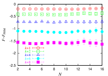
where $\mathrm{Ai}(x)$ is the Airy function and the type of correction ${\rm O}(e^{-2\pi\sqrt{\lambda}})$ is neglected. In fig. 2 (Left) we plot our results for $N=4$ and compare them with the FHM result (18). We find that our result agrees reasonably well with the FHM result in the strong coupling regime. To see more precisely, we plot in fig. 2 (Right) the difference between our result and the FHM result against $N$ for various $k$. It turns out that there are discrepancies which are almost independent of $N$. This strongly suggests that the FHM result correctly incorporates the finite $N$ effects except for a term which depends only on $k$. Note that this discrepancy cannot be explained by the worldsheet instanton effect ${\rm O}(e^{-2\pi\sqrt{\lambda}})$, which is neglected in FHM. See ref. [7] for a natural interpretation of this discrepancy from topological string theory.

In this paper we have established a simple numerical method for studying the ABJM theory on a three sphere for arbitrary rank $N$ and arbitrary Chern-Simons level $k$. The crucial point is that we are able to rewrite the ABJM matrix model, which is obtained after applying the localization technique, in such a way that the integrand becomes positive definite. By using this method, we have confirmed from first principles that the free energy in the M-theory limit grows proportionally to $N^{3/2}$ as predicted from the eleven-dimensional supergravity. We have also found that the FHM formula with the additional terms describes the free energy of the ABJM theory in the type IIA superstring and M-theory regimes. While we have focused on the free energy as the most fundamental quantity in the ABJM theory, our method can be used to calculate the expectation values of BPS operators. For instance, it is possible to calculate the expectation value of the circular Wilson loop for various representations [19].

We hope that the results of this work are convincing enough to show the power of the combination of the localization method and numerical simulation. We expect further numerical study of various localized matrix models will reveal exciting new aspects of supersymmetric gauge theories and quantum gravity.

References

- [1] J. Giedt, Int. J. Mod. Phys. A 24, 4045 (2009).
- [2] M. Hanada, J. Nishimura and S. Takeuchi, Phys. Rev. Lett. 99, 161602 (2007).
- [3] T. Eguchi and H. Kawai, Phys. Rev. Lett. 48, 1063 (1982).
- [4] T. Ishii, G. Ishiki, S. Shimasaki and A. Tsuchiya. Phys. Rev. D 78, 106001 (2008).
- [5] M. Hanada, S. Matsuura and F. Sugino, Prog. Theor. Phys. 126, 597 (2011).
- [6] V. Pestun, Commun. Math. Phys. 313, 71 (2012).
- [7] M. Hanada, M. Honda, Y. Honma, J. Nishimura, S. Shiba and Y. Yoshida, JHEP 1205, 121 (2012).
- [8] O. Aharony, O. Bergman, D. L. Jafferis and J. Maldacena, JHEP 0810 (2008) 091.
- [9]
A. Kapustin, B. Willett and I. Yaakov,
JHEP 1003 (2010) 089,
D. L. Jafferis, JHEP 1205, 159 (2012),
N. Hama, K. Hosomichi and S. Lee, JHEP 1103, 127 (2011). - [10]
M. Honda, G. Ishiki, J. Nishimura and A. Tsuchiya,
PoS LAT 2011, 244 (2011),
J. Nishimura, PoS LAT 2009, 016 (2009),
M. Honda, G. Ishiki, S. -W. Kim, J. Nishimura and A. Tsuchiya, PoS LATTICE 2010, 253 (2010). - [11]
J. K. Erickson, G. W. Semenoff and K. Zarembo,
Nucl. Phys. B 582, 155 (2000),
N. Drukker and D. J. Gross, J. Math. Phys. 42, 2896 (2001). - [12] W. Bietenholz and J. Nishimura, JHEP 0107, 015 (2001).
- [13]
M. Hanada, L. Mannelli and Y. Matsuo,
JHEP 0911, 087 (2009) ,
M. Honda and Y. Yoshida, Nucl. Phys. B 865, 21 (2012),
Y. Asano, G. Ishiki, T. Okada and S. Shimasaki, Phys. Rev. D 85, 106003 (2012). - [14] A. Kapustin, B. Willett and I. Yaakov, JHEP 1010, 013 (2010).
- [15] C. P. Herzog, I. R. Klebanov, S. S. Pufu and T. Tesileanu, Phys. Rev. D 83, 046001 (2011).
- [16] M. Marino and P. Putrov, J. Stat. Mech. 1203, P03001 (2012).
- [17] N. Drukker, M. Mariño and P. Putrov, Commun. Math. Phys. 306 (2011) 511.
- [18] H. Fuji, S. Hirano and S. Moriyama, JHEP 1108 (2011) 001.
- [19] M. Hanada, M. Honda, Y. Honma, J. Nishimura, S. Shiba and Y. Yoshida, in preparation.