跳到论文正文
W Papers独立论文阅读器 arXiv:1211.6827 论文正文 计算阅读时间 · 0%
引用这篇论文根据当前论文元数据生成,正式投稿前建议核对。


License: arXiv.org perpetual non-exclusive license
arXiv:1211.6827v1 [eess.SY] 29 Nov 2012

Additive-State-Decomposition-Based Tracking Control for TORA Benchmark

Quan Quan    Kai-Yuan Cai ††thanks: The authors are with Department of Automatic Control, Beijing University of Aeronautics and Astronautics, Beijing 100191, China. Q. Quan, Assistant Professor (Lecturer), qq_buaa@buaa.edu.cn, http://quanquan.buaa.edu.cn. K.-Y. Cai, Professor, kycai@buaa.edu.cn.
Abstract

In this paper, a new control scheme, called additive-state-decomposition-based tracking control, is proposed to solve the tracking (rejection) problem for rotational position of the TORA (a nonlinear nonminimum phase system). By the additive state decomposition, the tracking (rejection) task for the considered nonlinear system is decomposed into two independent subtasks: a tracking (rejection) subtask for a linear time invariant (LTI) system, leaving a stabilization subtask for a derived nonlinear system. By the decomposition, the proposed tracking control scheme avoids solving regulation equations and can tackle the tracking (rejection) problem in the presence of any external signal (except for the frequencies at ±1\pm 1) generated by a marginally stable autonomous LTI system. To demonstrate the effectiveness, numerical simulation is given.

Index Terms: 
TORA, RTAC, Nonminimum phase, Additive state decomposition.

I Introduction

The tracking (rejection) problem for a nonlinear benchmark system called translational oscillator with a rotational actuator (TORA) and also known as rotational-translational actuator (RTAC) has received a considerable amount of attention these years [1]-[8]. Some results were presented concerning the tracking (rejection) problem for general external signals [2],[3]. However, the proposed control methods cannot achieve asymptotic disturbance rejection. Taking this into account, the nonlinear output regulation theory was applied to track (reject) external signals generated by an autonomous system. In this case, asymptotic disturbance rejection can be achieved. By using different measurement, the tracking (rejection) problem for translational displacement of the TORA were investigated [4]-[6]. Readers can refer to [6] for details. Based on the same benchmark system, some other work was also presented concerning the tracking (rejection) problem for rotational position by nonlinear output regulation theory [7],[8]. For the two types of tracking (rejection) problems, regulator equations have to be solved and then the resulting solutions will be further used in the controller design. However, the difficulty of constructing and solving regulator equations will increase as the complexity of external signals increases. Moreover, it may fail to design a controller if regulator equations have no solutions. These are our major motivation.

In this paper, the tracking (rejection) problem for rotational position of the TORA as [7],[8] is revisited by a new control scheme called additive-state-decomposition-based tracking control, which is based on the additive state decomposition11 1 In this paper we have replaced the term “additive decomposition” in [9] with the more descriptive term “additive state decomposition”.. The proposed additive state decomposition is a new decomposition manner different from the lower-order subsystem decomposition methods. Concretely, taking the system x˙​(t)=f⁡(t,x),x∈ℝn\dot{x}\left(t\right)=f\left(t,x\right),x\in\mathbb{R}^{n} for example, it is decomposed into two subsystems: x˙1​(t)=f1​(t,x1,x2)\dot{x}_{1}\left(t\right)=f_{1}\left(t,x_{1},x_{2}\right) and x˙2​(t)=f2​(t,x1,x2)\dot{x}_{2}\left(t\right)=f_{2}\left(t,x_{1},x_{2}\right), where x1∈ℝn1x_{1}\in\mathbb{R}^{n_{1}}\ andx2∈ℝn2,\ x_{2}\in\mathbb{R}^{n_{2}}, respectively. The lower-order subsystem decomposition satisfies

n=n1+n2​ and ​x=x1⊕x2.n=n_{1}+n_{2}\text{ and }x=x_{1}\oplus x_{2}.

By contrast, the proposed additive state decomposition satisfies

n=n1=n2​ and​x=x1+x2.n=n_{1}=n_{2}\text{ and}\ x=x_{1}+x_{2}.

In our opinion, lower-order subsystem decomposition aims to reduce the complexity of the system itself, while the additive state decomposition emphasizes the reduction of the complexity of tasks for the system.

By following the philosophy above, the original tracking (rejection) task is ‘additively’ decomposed into two independent subtasks, namely the tracking (rejection) subtask for a linear time invariant (LTI) system and the stabilization subtask for a derived nonlinear system. Since tracking (rejection) subtask only needs to be achieved on an LTI system, the complexity of external signals can be handled easier by the transfer function method. It is proved that the designed controller can tackle the tracking (rejection) problem for rotational position of the TORA in the presence of any external signal (except for the frequency at ±1\pm 1) generated by a marginally stable autonomous LTI system.

This paper is organized as follows. In Section 2, the problem is formulated and the additive state decomposition is recalled briefly first. In Section 3, an observer is proposed to compensate for nonlinearity; then the resulting system is ‘additively’ decomposed into two subsystems; sequently, controllers are designed for them. In Section 4, numerical simulation is given. Section 5 concludes this paper.

II Nonlinear Benchmark Problem and Additive State Decomposition

II-A Nonlinear Benchmark Problem

As shown in Fig.1, the TORA system consists of a cart attached to a wall with a spring. The cart is affected by a disturbance force FF. An unbalanced point mass rotates around the axis in the center of the cart, which is actuated by a control torque N.N. The translational displacement of the cart is denoted by xcx_{c} and the rotational position of the unbalanced point mass is denoted by θ.\theta.

Refer to caption
Fig. 1: TORA system configuration [1]

For simplicity, after normalization and transformation, the TORA system is described by the following state-space representation [1]:

x˙1\displaystyle\dot{x}_{1} =x2\displaystyle=x_{2} (1a)
x˙2\displaystyle\dot{x}_{2} =−x1+εsinx3+Fd\displaystyle=-x_{1}+\varepsilon\sin x_{3}+F_{d} (1b)
x˙3\displaystyle\dot{x}_{3} =x4\displaystyle=x_{4} (1c)
x˙4\displaystyle\dot{x}_{4} =u−εcosx31−ε2​cos2⁡x3​Fd,x⁡(0)=x0\displaystyle=u-\frac{\varepsilon\cos x_{3}}{1-\varepsilon^{2}\cos^{2}x_{3}}F_{d},x\left(0\right)=x_{0} (1d)
where 0<ε<1,0<\varepsilon<1, x=[x1x2x3x4]T∈ℝ4x=[\begin{array}[c]{cccc}x_{1}&x_{2}&x_{3}&x_{4}\end{array}]^{T}\in\mathbb{R}^{4}, x3=θx_{3}=\theta, Fd∈ℝF_{d}\in\mathbb{R} is the unknown dimensionless disturbance, u∈ℝu\in\mathbb{R} is the dimensionless control torque. In this paper, the tracking (rejection) problem for rotational position of the TORA as [7],[8] is revisited. Concretely, for system (1), it is to design a controller uu such that the output y⁡(t)=x3​(t)→ry\left(t\right)=x_{3}\left(t\right)\rightarrow r as t→∞,t\rightarrow\infty, meanwhile keeping the other states bounded, where r∈(−π/2,π/2)r\in(-\pi\left/2\right.,\pi\left/2\right.) is a known constant. Obviously, this is a nonlinear nonminimum phase tracking problem, or say a nonlinear weakly minimum phase tracking problem. For system (1), the following assumptions are imposed.

Assumption 1. The state xx can be obtained.

Assumption 2. The disturbance Fd∈ℝF_{d}\in\mathbb{R} is generated by an autonomous LTI system

w˙=S​w,Fd=CdT​w\dot{w}=Sw,F_{d}=C_{d}^{T}w (2)

where S=−ST∈ℝm×mS=-S^{T}\in\mathbb{R}^{m\times m}, Cd∈ℝmC_{d}\in\mathbb{R}^{m} are constant matrix, w∈ℝm,w\in\mathbb{R}^{m}, and the pair (CdT,S)\left(C_{d}^{T},S\right) is observable.

Remark 1. If all eigenvalues of SS have zero real part, then, in suitable coordinates, the matrix SS can always be written to be a skew-symmetric matrix. The matrix SS in previous literature on the output regulation problem is often chosen in a simple form S=[0ω−ω0],S=\left[\begin{array}[c]{cc}0&\omega\\ -\omega&0\end{array}\right], where ω\omega is a positive real [4]-[8]. In such a case, FdF_{d} is in the form as sin(±ω​t)\left(\pm\omega t\right) and the solution to the regulator equation is easier to obtain. However, this is a difficulty when SS is complicated.

II-B Additive State Decomposition

In order to make the paper self-contained, the additive state decomposition [9] is recalled here briefly. Consider the following ‘original’ system:

f⁡(t,x˙,x)=0,x⁡(0)=x0f\left({t,\dot{x},x}\right)=0,x\left(0\right)=x_{0} (3)

where x∈ℝnx\in\mathbb{R}^{n}. We first bring in a ‘primary’ system having the same dimension as (3), according to:

fp(t,x˙p,xp)=0,x(0)p=xp,0f_{p}\left({t,\dot{x}_{p},x_{p}}\right)=0,x{{}_{p}}\left(0\right)=x_{p,0} (4)

where xp∈ℝn{x_{p}}\in\mathbb{R}^{n}. From the original system (3) and the primary system (4) we derive the following ‘secondary’ system:

f⁡(t,x˙,x)−fp​(t,x˙p,xp)=0,x⁡(0)=x0f\left({t,\dot{x},x}\right)-f_{p}\left({t,\dot{x}_{p},x_{p}}\right)=0,x\left(0\right)=x_{0} (5)

where xp∈ℝn{x_{p}}\in\mathbb{R}^{n} is given by the primary system (4). Define a new variable xs∈ℝn{x_{s}}\in\mathbb{R}^{n} as follows:

xs≜x−xp.{x_{s}\triangleq x-x_{p}}. (6)

Then the secondary system (5) can be further written as follows:

f(t,x˙s+x˙p,xs+xp)−fp(t,x˙p,xp)=0,x(0)s=x0−xp,0.f\left({t,\dot{x}_{s}+\dot{x}_{p},x_{s}+x_{p}}\right)-f_{p}\left({t,\dot{x}_{p},x_{p}}\right)=0,x{{}_{s}}\left(0\right)=x_{0}-x_{p,0}. (7)

From the definition (6), we have

x⁡(t)=xp​(t)+xs​(t),t≥0.{x}\left(t\right)={x_{p}\left(t\right)+x_{s}\left(t\right),t\geq 0.} (8)

Remark 2. By the additive state decomposition, the system (3) is decomposed into two subsystems with the same dimension as the original system. In this sense our decomposition is “additive”. In addition, this decomposition is with respect to state. So, we call it “additive state decomposition”.

As a special case of (3), a class of differential dynamic systems is considered as follows:

x˙\displaystyle\dot{x} =f⁡(t,x),x⁡(0)=x0,\displaystyle=f\left({t,x}\right),x\left(0\right)=x_{0},
y\displaystyle y =h⁡(t,x)\displaystyle=h\left({t,x}\right) (9)

where x∈ℝn{x}\in\mathbb{R}^{n} and y∈ℝm.y\in\mathbb{R}^{m}. Two systems, denoted by the primary system and (derived) secondary system respectively, are defined as follows:

x˙p\displaystyle\dot{x}_{p} =fp​(t,xp),xp​(0)=xp,0\displaystyle=f_{p}\left({t,x_{p}}\right),x_{p}\left(0\right)=x_{p,0}
yp\displaystyle y_{p} =hp​(t,xp)\displaystyle=h_{p}\left({t,x}_{p}\right) (10)

and

x˙s\displaystyle\dot{x}_{s} =f⁡(t,xp+xs)−fp​(t,xp),xs​(0)=x0−xp,0,\displaystyle=f\left({t,x_{p}}+{x_{s}}\right)-f_{p}\left({t,x_{p}}\right),x_{s}\left(0\right)=x_{0}-x_{p,0},
ys\displaystyle y_{s} =h⁡(t,xp+xs)−hp​(t,xp)\displaystyle=h\left({t,x_{p}}+{x_{s}}\right)-h_{p}\left({t,x}_{p}\right) (11)

where xs≜x−xp{x_{s}}\triangleq{x-x_{p}} and ys≜y−ypy_{s}\triangleq{y-y_{p}}. The secondary system (11) is determined by the original system (9) and the primary system (10). From the definition, we have

x⁡(t)=xp​(t)+xs​(t),y⁡(t)=yp​(t)+ys​(t),t≥0.{x}\left(t\right)={x_{p}\left(t\right)+x_{s}\left(t\right),y\left(t\right)=y_{p}\left(t\right)+y_{s}\left(t\right),t\geq 0.} (12)

III Additive-State-Decomposition-Based Tracking Control

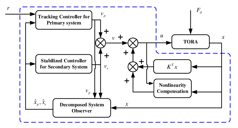
In this section, in order to decrease nonlinearity, an observer is proposed to compensate for the nonlinear term εcosx31−ε2​cos2⁡x3​Fd.\frac{\varepsilon\cos x_{3}}{1-\varepsilon^{2}\cos^{2}x_{3}}F_{d}. After the compensation, the resulting nonlinear nonminimum phase tracking system is decomposed into two systems by the additive state decomposition: an LTI system including all external signals as the primary system, leaving the secondary system with a zero equilibrium point. Therefore, the tracking problem for the original system is correspondingly decomposed into two subproblems by the additive state decomposition: a tracking problem for the LTI ‘primary’ system and a stabilization problem for the secondary system. Obviously, the two subproblems are easier than the original one. Therefore, the original tracking problem is simplified. The structure of the closed-loop system is shown in Fig.2.
Refer to caption
Fig. 2: Structure of the closed-loop system

III-A Nonlinearity Compensation

First, in order to estimate the termεcosx31−ε2​cos2⁡x3​Fd,\frac{\varepsilon\cos x_{3}}{1-\varepsilon^{2}\cos^{2}x_{3}}F_{d}, an observer is designed, which is stated in Theorem 1.

Theorem 1. Under Assumptions 1-2, for system (1), let the observer be designed as follows

w^˙\displaystyle\dot{\hat{w}} =S​w^+l1​εcosx31−ε2​cos2⁡x3​Cd​(x^4−x4)\displaystyle=S\hat{w}+l_{1}\frac{\varepsilon\cos x_{3}}{1-\varepsilon^{2}\cos^{2}x_{3}}C_{d}\left(\hat{x}_{4}-x_{4}\right)
x^˙4\displaystyle\dot{\hat{x}}_{4} =−l2​(x^4−x4)−l1​εcosx31−ε2​cos2⁡x3​CdT​w^+u\displaystyle=-l_{2}\left(\hat{x}_{4}-x_{4}\right)-l_{1}\frac{\varepsilon\cos x_{3}}{1-\varepsilon^{2}\cos^{2}x_{3}}C_{d}^{T}\hat{w}+u (13)
F^d\displaystyle\hat{F}_{d} =l1​CdT​w^,w^​(0)=0,x^4​(0)=0\displaystyle=l_{1}C_{d}^{T}\hat{w},\hat{w}\left(0\right)=0,\hat{x}_{4}\left(0\right)=0

where l1,l2>0.l_{1},l_{2}>0. Then limt→∞​εcosx31−ε2​cos2⁡x3​F~d​(t)=0,\underset{t\rightarrow\infty}{\lim}\frac{\varepsilon\cos x_{3}}{1-\varepsilon^{2}\cos^{2}x_{3}}\tilde{F}_{d}\left(t\right)=0, where F~d≜F^d−Fd.\tilde{F}_{d}\triangleq\hat{F}_{d}-F_{d}.

Proof. See Appendix A. □\square

By using the observer (13), the controller uu in (1) is designed as follows

u=KT​x+v+εcosx31−ε2​cos2⁡x3​F^du=K^{T}x+v+\frac{\varepsilon\cos x_{3}}{1-\varepsilon^{2}\cos^{2}x_{3}}\hat{F}_{d}

where K∈ℝ4K\in\mathbb{R}^{4} and v∈ℝv\in\mathbb{R} will be specified later. Then the system (1) becomes

x˙1\displaystyle\dot{x}_{1} =x2\displaystyle=x_{2}
x˙2\displaystyle\dot{x}_{2} =−x1+εsinx3+Fd\displaystyle=-x_{1}+\varepsilon\sin x_{3}+F_{d}
x˙3\displaystyle\dot{x}_{3} =x4\displaystyle=x_{4}
x˙4\displaystyle\dot{x}_{4} =KT​x+v+εcosx31−ε2​cos2⁡x3​F~d,x⁡(0)=x0.\displaystyle=K^{T}x+v+\frac{\varepsilon\cos x_{3}}{1-\varepsilon^{2}\cos^{2}x_{3}}\tilde{F}_{d},x\left(0\right)=x_{0}. (14)

III-B Additive State Decomposition of Original System

Introduce a zero term ε​D​(C+a​B)T​x−ε⁡(y+a​y˙)=0\varepsilon D\left(C+aB\right)^{T}x-\varepsilon\left(y+a\dot{y}\right)=0\ into the system (14), where a>0,a>0, B=[0001]TB=[\begin{array}[c]{cccc}0&0&0&1\end{array}]^{T}, C=[0010]TC=[\begin{array}[c]{cccc}0&0&1&0\end{array}]^{T}\ and (C+a​B)T​x=y+a​y˙.\left(C+aB\right)^{T}x=y+a\dot{y}. Then the system (14) becomes

x˙\displaystyle\dot{x} =A​x+B​v+ϕ⁡(y,y˙)+D​Fd+φ\displaystyle=Ax+Bv+\phi\left(y,\dot{y}\right)+DF_{d}+\varphi
y\displaystyle y =CT​x,x⁡(0)=x0\displaystyle=C^{T}x,x\left(0\right)=x_{0} (15)

where

A0\displaystyle A_{0} =[0100−100000010000],A=A0+B​KT+ε​D​(C+a​B)T,\displaystyle=\left[\begin{array}[c]{cccc}0&1&0&0\\ -1&0&0&0\\ 0&0&0&1\\ 0&0&0&0\end{array}\right],A=A_{0}+BK^{T}+\varepsilon D\left(C+aB\right)^{T},
D\displaystyle D =[0100],ϕ⁡(y,y˙)=[0ε​sin⁡y−ε⁡(y+a​y˙)00],φ=[000εcosx31−ε2​cos2⁡x3​F~d].\displaystyle=\left[\begin{array}[c]{c}0\\ 1\\ 0\\ 0\end{array}\right],\phi\left(y,\dot{y}\right)=\left[\begin{array}[c]{c}0\\ \varepsilon\sin y-\varepsilon\left(y+a\dot{y}\right)\\ 0\\ 0\end{array}\right],\varphi=\left[\begin{array}[c]{c}0\\ 0\\ 0\\ \frac{\varepsilon\cos x_{3}}{1-\varepsilon^{2}\cos^{2}x_{3}}\tilde{F}_{d}\end{array}\right].

The additive state decomposition is ready to apply to the system (15), for which the primary system is chosen to be an LTI system including all external signals as follows

x˙p\displaystyle\dot{x}_{p} =A​xp+B​vp+d+φ\displaystyle=Ax_{p}+Bv_{p}+d+\varphi
yp\displaystyle y_{p} =CT​xp,xp​(0)=x0\displaystyle=C^{T}x_{p},x_{p}\left(0\right)=x_{0} (32)

where d=ϕ⁡(r,0)+D​Fd.d=\phi\left(r,0\right)+DF_{d}. Then, according to the rule (11), the secondary system is derived from the original system (15) and the primary system (32) as follows

x˙s\displaystyle\dot{x}_{s} =A​xs+B​vs+ϕ⁡(yp+ys,y˙p+y˙s)−ϕ⁡(r,0)\displaystyle=Ax_{s}+Bv_{s}+\phi\left(y_{p}+y_{s},\dot{y}_{p}+\dot{y}_{s}\right)-\phi\left(r,0\right)
ys\displaystyle y_{s} =CT​xs,xs​(0)=0\displaystyle=C^{T}x_{s},x_{s}\left(0\right)=0 (33)

where vs=v−vp.v_{s}=v-v_{p}. According to (12), we have

x=xp+xs​and ​y=yp+ys.x=x_{p}+x_{s}\ \text{and }y=y_{p}+y_{s}. (34)

Remark 3. The pair (A0,B)\left(A_{0},B\right) is uncontrollable, while the pair (A0+ε​D​(C+a​B)T,B)\left(A_{0}+\varepsilon D\left(C+aB\right)^{T},B\right) is controllable. Therefore, there always exists a vectorK\ K such that A=A0+B​KT+ε​D​(C+a​B)TA=A_{0}+BK^{T}+\varepsilon D\left(C+aB\right)^{T} is a stable matrix.

Remark 4. If yp≡ry_{p}\equiv r and y˙p≡0,\dot{y}_{p}\equiv 0, then (xs,vs)=0\left(x_{s},v_{s}\right)=0 is a zero equilibrium point of the secondary system (33).

So far, the nonlinear nonminimum phase tracking system (15) is decomposed into two systems by the additive state decomposition, where the external signal d+φd+\varphi is shifted to (32) and the nonlinear term ϕ⁡(⋅)\phi\left(\cdot\right) is shifted to (33). The strategy here is to assign the tracking (rejection) task to the primary system (32) and stabilization task to the secondary system (33). More concretely, in (32) design vpv_{p} to track rr, and design vsv_{s} to stabilize (33). If so, by the relationship (34), yy can track r.r. In the following, controllers vpv_{p} and vsv_{s} are designed separately.

III-C Tracking Controller Design for Primary System

Before proceeding further, we have the following preliminary result.

Consider the following linear system

z˙1\displaystyle\dot{z}_{1} =Sz​z1+A12​ez\displaystyle=S_{z}z_{1}+A_{12}e_{z}
z˙2\displaystyle\dot{z}_{2} =A21​z1+A22​z2+d1+φ1\displaystyle=A_{21}z_{1}+A_{22}z_{2}+d_{1}+\varphi_{1}
ez\displaystyle e_{z} =CeT​z2+d2+φ2,z⁡(0)=z0\displaystyle=C_{e}^{T}z_{2}+d_{2}+\varphi_{2},z\left(0\right)=z_{0} (35)

where Sz∈ℝm1×m1S_{z}\in\mathbb{R}^{m_{1}\times m_{1}} is a marginally stable matrix, A12∈ℝm1,A_{12}\in\mathbb{R}^{m_{1}}, Ce∈ℝm2,C_{e}\in\mathbb{R}^{m_{2}}, A21∈ℝm2×m2,A_{21}\in\mathbb{R}^{m_{2}\times m_{2}}, A22∈ℝm2×m1,A_{22}\in\mathbb{R}^{m_{2}\times m_{1}}, z1∈ℝm1,z_{1}\in\mathbb{R}^{m_{1}}, z2,d1,φ1∈ℝm2,z_{2},d_{1},\varphi_{1}\in\mathbb{R}^{m_{2}}, z=[z1Tz2T]T∈ℝm1+m2z=[\begin{array}[c]{cc}z_{1}^{T}&z_{2}^{T}\end{array}]^{T}\in\mathbb{R}^{m_{1}+m_{2}} and ez,d2,φ2∈ℝ.e_{z},d_{2},\varphi_{2}\in\mathbb{R}.

Lemma 1. Suppose i) φi​(t)\varphi_{i}\left(t\right) is bounded on [0,∞)\left[0,\infty\right) andlimt→∞‖φi(t)‖=0,i=1,2,\ \underset{t\rightarrow\infty}{\lim}\left\|\varphi_{i}\left(t\right)\right\|=0,i=1,2, ii) every element of d1​(t),d2​(t)d_{1}\left(t\right),d_{2}\left(t\right) are bounded on [0,∞)\left[0,\infty\right) and can be generated by w˙z=Sz​wz,\dot{w}_{z}=S_{z}w_{z}, dz=CzT​wzd_{z}=C_{z}^{T}w_{z}\ with appropriate initial values, where Cz∈ℝm1,C_{z}\in\mathbb{R}^{m_{1}}, iii) the parameters in (35) satisfy

max⁡Re⁡λ⁡(Az)<0,Az=[SzA12​CeTA21A22].\max\operatorname{Re}\lambda\left(A_{z}\right)<0,A_{z}=\left[\begin{array}[c]{cc}S_{z}&A_{12}C_{e}^{T}\\ A_{21}&A_{22}\end{array}\right]. (36)

Then in (35) limt→∞​ez​(t)=0,\underset{t\rightarrow\infty}{\lim}e_{z}\left(t\right)=0, meanwhile keeping z1​(t)z_{1}\left(t\right) and z2​(t)z_{2}\left(t\right) bounded.

Proof. See Appendix B. □\square

Define a filtered tracking error to be

ep=y~p+a​y~˙p=(C+a​B)T​xp−re_{p}=\tilde{y}_{p}+a\dot{\tilde{y}}_{p}=\left(C+aB\right)^{T}x_{p}-r (37)

where y~p=yp−r,\tilde{y}_{p}=y_{p}-r, r˙=0\dot{r}=0 and a>0a>0. Let us consider the tracking problem for the primary system (32). With Lemma 1 in hand, the design of vpv_{p} is stated in Theorem 2.

Theorem 2. For the primary system (32), let the controller vpv_{p} be designed as follows

ξ˙\displaystyle\dot{\xi} =Sa​ξ+L1​ep\displaystyle=S_{a}\xi+L_{1}e_{p}
vp​(ξ,xp,r)\displaystyle v_{p}\left(\xi,x_{p},r\right) =L2T​xp+L3T​ξ\displaystyle=L_{2}^{T}x_{p}+L_{3}^{T}\xi (38)

where Sa=S_{a}=diag(0,S),\left(0,S\right), L1∈ℝm+1,L2∈ℝ4L_{1}\in\mathbb{R}^{m+1},L_{2}\in\mathbb{R}^{4} and L3∈ℝm+1L_{3}\in\mathbb{R}^{m+1} satisfy

max⁡Re⁡λ⁡(Aa)<0,Aa=[SaL1​(C+a​B)TB​L3TA+B​L2T].\max\operatorname{Re}\lambda\left(A_{a}\right)<0,A_{a}=\left[\begin{array}[c]{cc}S_{a}&L_{1}\left(C+aB\right)^{T}\\ BL_{3}^{T}&A+BL_{2}^{T}\end{array}\right]. (39)

Then limt→∞​yp​(t)=r\underset{t\rightarrow\infty}{\lim}y_{p}\left(t\right)=r\ andlimt→∞​y˙p​(t)=0\ \underset{t\rightarrow\infty}{\lim}\dot{y}_{p}\left(t\right)=0 meanwhile keeping xp​(t)x_{p}\left(t\right) andξ⁡(t)\ \xi\left(t\right) bounded.

Proof. Incorporating the controller (38) into the primary system (32) results in

ξ˙\displaystyle\dot{\xi} =Sa​ξ+L1​ep\displaystyle=S_{a}\xi+L_{1}e_{p}
x˙p\displaystyle\dot{x}_{p} =(A+B​L2T)​xp+B​L3T​ξ+d+φ\displaystyle=\left(A+BL_{2}^{T}\right)x_{p}+BL_{3}^{T}\xi+d+\varphi
ep\displaystyle e_{p} =(C+a​B)T​xp−r\displaystyle=\left(C+aB\right)^{T}x_{p}-r

where the definition (37) is utilized. Moreover, every element of dd\ andr\ r\ can be generated by an autonomous system in the form w˙a=Sa​wa,da=CaT​wa\dot{w}_{a}=S_{a}w_{a},d_{a}=C_{a}^{T}w_{a}\ with appropriate initial values, where Ca=[1CdT]T.C_{a}=[\begin{array}[c]{cc}1&C_{d}^{T}\end{array}]^{T}. By Lemma 1, if (39) holds, then limt→∞​ep​(t)=0\underset{t\rightarrow\infty}{\lim}e_{p}\left(t\right)=0 meanwhile keeping xp​(t)x_{p}\left(t\right) andξ⁡(t)\ \xi\left(t\right) bounded. It is easy to see from (37) that both y~p\tilde{y}_{p} and y~˙p\dot{\tilde{y}}_{p} can be viewed as outputs of a stable system with epe_{p} as input. This means that y~p\tilde{y}_{p} and y~˙p\dot{\tilde{y}}_{p} are bounded if epe_{p} is bounded. In addition, limt→∞​y~p​(t)=0\underset{t\rightarrow\infty}{\lim}\tilde{y}_{p}\left(t\right)=0\ andlimt→∞​y~˙p​(t)=0.\ \underset{t\rightarrow\infty}{\lim}\dot{\tilde{y}}_{p}\left(t\right)=0. □\square

In most of cases, the controller parameters L1,L2L_{1},L_{2} and L3L_{3} in (38) can be always found. This is shown in the following proposition.

Proposition 1. For any S=−STS=-S^{T} without eigenvalues ±j,\pm j, the parameters

L1=[1CdT]T,L2=−1a​C−B−1a​H−1a​K,L3=−1a​L1L_{1}=[\begin{array}[c]{cc}1&C_{d}^{T}\end{array}]^{T},L_{2}=-\frac{1}{a}C-B-\frac{1}{a}H-\frac{1}{a}K,L_{3}=-\frac{1}{a}L_{1} (40)

can always make max⁡Re⁡λ⁡(Aa)<0,\max\operatorname{Re}\lambda\left(A_{a}\right)<0, where H=[0ε01]T.H=[\begin{array}[c]{cccc}0&\varepsilon&0&1\end{array}]^{T}.

Proof. See Appendix C. □\square

Remark 5. Proposition 1 in fact implies that, in the presence of any external signal (except for the frequencies at ±1\pm 1), the controller (38) with parameters (40) can always make limt→∞​yp​(t)=r\underset{t\rightarrow\infty}{\lim}y_{p}\left(t\right)=r\ andlimt→∞​y˙p​(t)=0\ \underset{t\rightarrow\infty}{\lim}\dot{y}_{p}\left(t\right)=0 meanwhile keeping xp​(t)x_{p}\left(t\right) andξ⁡(t)\ \xi\left(t\right) bounded. In other words, the disturbance like sin⁡t\sin t cannot be dealt with, which is consistent with [7]. If the external signal contains the component with frequencies at ±1,\pm 1, then such a frequency component can be chosen not to compensate for, i.e., SaS_{a} in (38) will not contain eigenvalues ±j\pm j.

III-D Stabilized Controller Design for Secondary System

So far, we have designed the tracking controller for the primary system (32). In this section, we are going to design the stabilized controller for the secondary system (33). It can be rewritten as

x˙1,s\displaystyle\dot{x}_{1,s} =x2,s\displaystyle=x_{2,s}
x˙2,s\displaystyle\dot{x}_{2,s} =−x1,s+ε​sin⁡(x3,s+r)−ε​sin⁡r+g\displaystyle=-x_{1,s}+\varepsilon\sin\left(x_{3,s}+r\right)-\varepsilon\sin r+g
x˙3,s\displaystyle\dot{x}_{3,s} =x4,s\displaystyle=x_{4,s}
x˙4,s\displaystyle\dot{x}_{4,s} =KT​xs+vs,xs​(0)=0\displaystyle=K^{T}x_{s}+v_{s},x_{s}\left(0\right)=0 (41)

where g=ε​sin⁡(yp+x3,s)−ε​sin⁡(r+x3,s)−ε⁡(yp+a​y˙p−r).g=\varepsilon\sin\left(y_{p}+x_{3,s}\right)-\varepsilon\sin\left(r+x_{3,s}\right)-\varepsilon\left(y_{p}+a\dot{y}_{p}-r\right). Our constructive procedure has been inspired by the design in [3]. We will start the controller design procedure from the marginally stable (x1,s,x2,s)\left(x_{1,s},x_{2,s}\right)-subsystem.

Step 1. Consider the (x1,s,x2,s)\left(x_{1,s},x_{2,s}\right)-subsystem of (41) with x3,sx_{3,s} viewed as the virtual control input. Differentiating the quadratic function V1=12​(x1,s2+x2,s2)V_{1}=\frac{1}{2}\left(x_{1,s}^{2}+x_{2,s}^{2}\right) results in

V˙1=ε​x2,s​[sin⁡(x3,s+r)−sin⁡r]+ε​x2,s​g.\dot{V}_{1}=\varepsilon x_{2,s}\left[\sin\left(x_{3,s}+r\right)-\sin r\right]+\varepsilon x_{2,s}g. (42)

Guided by the state-feedback design [10], we introduce the following “Certainty Equivalence” (CE) based virtual controller

x3,s=−b​atan​x2,s+x3,s′.x_{3,s}=-b\text{atan}x_{2,s}+x_{3,s}^{\prime}. (43)

Then

x˙1,s\displaystyle\dot{x}_{1,s} =x2,s\displaystyle=x_{2,s}
x˙2,s\displaystyle\dot{x}_{2,s} =−x1,s+2​ε​sin⁡(−b​atan​x2,s2)​cos⁡(−b​atan​x2,s+2​r2)+g′\displaystyle=-x_{1,s}+2\varepsilon\sin\left(\frac{-b\text{atan}x_{2,s}}{2}\right)\cos\left(\frac{-b\text{atan}x_{2,s}+2r}{2}\right)+g^{\prime} (44)

where

g′=ε​sin⁡(r−b​atan​x2,s+x3,s′)−ε​sin⁡(r−b​atan​x2,s)+g.g^{\prime}=\varepsilon\sin\left(r-b\text{atan}x_{2,s}+x_{3,s}^{\prime}\right)-\varepsilon\sin\left(r-b\text{atan}x_{2,s}\right)+g. (45)

In order to ensure cos⁡(−b​atan​x2,s+2​r2)>0,\cos\left(\frac{-b\text{atan}x_{2,s}+2r}{2}\right)>0, the parameter bb is chosen to satisfy 0<b<2​(1−2​|r|/π).0<b<2\left(1-2\left|r\right|\left/\pi\right.\right). Since r∈(−π/2,π/2)r\in(-\pi\left/2\right.,\pi\left/2\right.) is a constant, bb always exists. The term CE is used here because x3,s′=0x_{3,s}^{\prime}=0 in (43) makes V˙1\dot{V}_{1} in (42) negative semidefinite as g≡0.g\equiv 0.

Step 2. We will apply backstepping to the (x3,s′,x4,s)\left(x_{3,s}^{\prime},x_{4,s}\right)-subsystem and design a nonlinear controller vsv_{s} to drive x3,s′x_{3,s}^{\prime} to the origin. By the definition (43), x3,s′=x3,s+bx_{3,s}^{\prime}=x_{3,s}+batanx2,s.x_{2,s}. Then the time derivative of the new variable x3,s′x_{3,s}^{\prime} is

x˙3,s′=x4,s+ψ+b​11+x2,s2​g\dot{x}_{3,s}^{\prime}=x_{4,s}+\psi+b\frac{1}{1+x_{2,s}^{2}}g (46)

where ψ=b​11+x2,s2​[−x1,s+ε​sin⁡(x3,s+r)−ε​sin⁡r].\psi=b\frac{1}{1+x_{2,s}^{2}}\left[-x_{1,s}+\varepsilon\sin\left(x_{3,s}+r\right)-\varepsilon\sin r\right]. Define a new variable x4,s′x_{4,s}^{\prime} as follows

x4,s′=x3,s′+x4,s+ψ.x_{4,s}^{\prime}=x_{3,s}^{\prime}+x_{4,s}+\psi. (47)

Then (46) becomes

x˙3,s′=−x3,s′+x4,s′+b​11+x2,s2​g.\dot{x}_{3,s}^{\prime}=-x_{3,s}^{\prime}+x_{4,s}^{\prime}+b\frac{1}{1+x_{2,s}^{2}}g.

By the definition (47), the time derivative of the new variable x4,s′x_{4,s}^{\prime} is

x˙4,s′\displaystyle\dot{x}_{4,s}^{\prime} =x˙3,s′+x˙4,s+ψ˙\displaystyle=\dot{x}_{3,s}^{\prime}+\dot{x}_{4,s}+\dot{\psi}
=−x3,s′+x4,s′+b​11+x2,s2​g+KT​xs+vs+ψ˙,\displaystyle=-x_{3,s}^{\prime}+x_{4,s}^{\prime}+b\frac{1}{1+x_{2,s}^{2}}g+K^{T}x_{s}+v_{s}+\dot{\psi},

where

ψ˙\displaystyle\dot{\psi} =−2​b​x2,s​1(1+x2,s2)2​[−x1,s+ε​sin⁡(x3,s+r)−ε​sin⁡r]\displaystyle=-2bx_{2,s}\frac{1}{\left(1+x_{2,s}^{2}\right)^{2}}\left[-x_{1,s}+\varepsilon\sin\left(x_{3,s}+r\right)-\varepsilon\sin r\right]
+b​11+x2,s2​[−x2,s+ε​cos⁡(x3,s+r)​x4,s].\displaystyle\text{ \ \ }+b\frac{1}{1+x_{2,s}^{2}}\left[-x_{2,s}+\varepsilon\cos\left(x_{3,s}+r\right)x_{4,s}\right].

Design vsv_{s} for the secondary system (41) as follows

vs​(xp,xs,r)=x3,s′−2​x4,s′−KT​xs−ψ˙.v_{s}\left(x_{p},x_{s},r\right)=x_{3,s}^{\prime}-2x_{4,s}^{\prime}-K^{T}x_{s}-\dot{\psi}. (48)

Then the (x3,s′,x4,s′)\left(x_{3,s}^{\prime},x_{4,s}^{\prime}\right)-subsystem becomes

x˙3,s′\displaystyle\dot{x}_{3,s}^{\prime} =−x3,s′+x4,s′+b​11+x2,s2​g\displaystyle=-x_{3,s}^{\prime}+x_{4,s}^{\prime}+b\frac{1}{1+x_{2,s}^{2}}g
x˙4,s′\displaystyle\dot{x}_{4,s}^{\prime} =−x4,s′+b​11+x2,s2​g.\displaystyle=-x_{4,s}^{\prime}+b\frac{1}{1+x_{2,s}^{2}}g. (49)

It is easy to see that limt→∞​x3,s′​(t)=0\underset{t\rightarrow\infty}{\lim}x_{3,s}^{\prime}\left(t\right)=0 and limt→∞​x4,s′​(t)=0\underset{t\rightarrow\infty}{\lim}x_{4,s}^{\prime}\left(t\right)=0\ as limt→∞​g​(t)=0.\underset{t\rightarrow\infty}{\lim}g\left(t\right)=0.

We are now ready to state the theorem for the secondary system.

Theorem 3. Suppose limt→∞​yp​(t)=r\underset{t\rightarrow\infty}{\lim}y_{p}\left(t\right)=r and limt→∞​y˙p​(t)=0.\underset{t\rightarrow\infty}{\lim}\dot{y}_{p}\left(t\right)=0. Let the controller vsv_{s} for the secondary system (41) be designed as (48), where 0<b<2​(1−2​|r|/π)0<b<2\left(1-2\left|r\right|\left/\pi\right.\right). Then limt→∞​‖xs​(t)‖=0\underset{t\rightarrow\infty}{\lim}\left\|x_{s}\left(t\right)\right\|=0 meanwhile keeping xs​(t)x_{s}\left(t\right) bounded.

Proof. See Appendix D. □\square

III-E Controller Synthesis for Original System

It should be noticed that the controller design above is based on the condition that xpx_{p} and xsx_{s} are known as priori. A problem arises that the states xpx_{p} and xsx_{s} cannot be measured directly except for x=xp+xsx=x_{p}+x_{s}. By taking this into account, the following observer is proposed to estimate the states xpx_{p} and xsx_{s}, which is stated in Theorem 4.

Theorem 4. Let the observer be designed as follows

x^˙s\displaystyle\dot{\hat{x}}_{s} =A​x^s+B​vs+ϕ⁡(y,y˙)−ϕ⁡(r,0)\displaystyle=A\hat{x}_{s}+Bv_{s}+\phi\left(y,\dot{y}\right)-\phi\left(r,0\right)
x^p\displaystyle\hat{x}_{p} =x−x^s,x^s​(0)=0\displaystyle=x-\hat{x}_{s},\hat{x}_{s}\left(0\right)=0 (50)

where AA is stable. Then x^p≡xp\hat{x}_{p}\equiv x_{p}\ and x^s≡xs.\hat{x}_{s}\equiv x_{s}.

Proof. Since x=xp+xs,x=x_{p}+x_{s}, we have y=yp+ys.y=y_{p}+y_{s}. Consequently, (50) can be rewritten as

x^˙s\displaystyle\dot{\hat{x}}_{s} =A​x^s+B​vs+ϕ⁡(yp+ys,y˙p+y˙s)−ϕ⁡(r,0)\displaystyle=A\hat{x}_{s}+Bv_{s}+\phi\left(y_{p}+y_{s},\dot{y}_{p}+\dot{y}_{s}\right)-\phi\left(r,0\right)
x^p\displaystyle\hat{x}_{p} =x−x^s,x^s​(0)=0.\displaystyle=x-\hat{x}_{s},\hat{x}_{s}\left(0\right)=0. (51)

Subtracting (33) from (51) results in

x~˙s=A​x~s,x~s​(0)=0\dot{\tilde{x}}_{s}=A\tilde{x}_{s},\tilde{x}_{s}\left(0\right)=0 (52)

where x~s=x^s−xs.\tilde{x}_{s}=\hat{x}_{s}-x_{s}. Then x^s≡xs.\hat{x}_{s}\equiv x_{s}. Furthermore, with the aid of the relationship xp=x−xs,x_{p}=x-x_{s}, we have x^p≡xp.□\hat{x}_{p}\equiv x_{p}.\ \square

Remark 6. Unlike traditional observers, the proposed observer can estimate the states of the primary system and the secondary system directly rather than asymptotically or exponentially. This can be explained that, although the initial value x0x_{0} is unknown, the initial value of either the primary system or the secondary system can be specified exactly, leaving an unknown initial value for the other system. The measurement xx and parameters may be inaccurate. In this case, it is expected that small uncertainties lead to x^p\hat{x}_{p}\ close to xpx_{p} (or x^s\hat{x}_{s}\ close to xsx_{s}). From (52), a stable matrix AA\ can ensure a small x~s\tilde{x}_{s} in the presence of small uncertainties.

Theorem 5. Suppose that the conditions of Theorems 1-4 hold. Let the controller uu in the system (1) be designed as follows

ξ˙\displaystyle\dot{\xi} =Sa​ξ+L1​[(C+a​B)T​x^p−r]\displaystyle=S_{a}\xi+L_{1}[\left(C+aB\right)^{T}\hat{x}_{p}-r]
u\displaystyle u =KT​x+vp​(ξ,x^p,r)+vs​(x^p,x^s,r)+εcosx31−ε2​cos2⁡x3​F^d\displaystyle=K^{T}x+v_{p}\left(\xi,\hat{x}_{p},r\right)+v_{s}\left(\hat{x}_{p},\hat{x}_{s},r\right)+\frac{\varepsilon\cos x_{3}}{1-\varepsilon^{2}\cos^{2}x_{3}}\hat{F}_{d} (53)

where F^d\hat{F}_{d} is given by (13), x^p\hat{x}_{p} and x^s\hat{x}_{s} are given by (50), vp​(⋅)v_{p}\left(\cdot\right) is defined in (38), and vs​(⋅)v_{s}\left(\cdot\right) is defined in (48). Then limt→∞​y​(t)=r\underset{t\rightarrow\infty}{\lim}y\left(t\right)=r meanwhile keeping xx\ and ξ\xi bounded.

Proof. Note that the original system (1), the primary system (32) and the secondary system (33) have the relationship: x=xp+xsx=x_{p}+x_{s} and y=yp+ys.y=y_{p}+y_{s}. With the controller (53), for the primary system (32), limt→∞​yp​(t)=r\underset{t\rightarrow\infty}{\lim}y_{p}\left(t\right)=r meanwhile keeping xpx_{p}\ andξ\ \xi bounded by Theorem 2. On the other hand, for the secondary system (33), we have limt→∞​xs​(t)=0\underset{t\rightarrow\infty}{\lim}x_{s}\left(t\right)=0\ meanwhile keeping xsx_{s} bounded on [0,∞)\left[0,\infty\right) by Theorem 3. In addition, Theorem 4 ensures that x^p≡xp\hat{x}_{p}\equiv x_{p}\ and x^s≡xs.\hat{x}_{s}\equiv x_{s}. Therefore, limt→∞​y​(t)=r\underset{t\rightarrow\infty}{\lim}y\left(t\right)=r meanwhile keeping xx\ and ξ\xi bounded. □\square

IV Numerical Simulation

In the simulation, set ε=0.2\varepsilon=0.2\ and the initial value x0=[0000]Tx_{0}=[\begin{array}[c]{cccc}0&0&0&0\end{array}]^{T}\ in (1). The unknown dimensionless disturbance FdF_{d} is generated by an autonomous LTI system (2) with the parameters as follows

S=[02−20],Cd=[10]T,w⁡(0)=[00.02]T.S=\left[\begin{array}[c]{cc}0&2\\ -2&0\end{array}\right],C_{d}=[\begin{array}[c]{cc}1&0\end{array}]^{T},w\left(0\right)=[\begin{array}[c]{cc}0&0.02\end{array}]^{T}.

The objective here is to design a controller uu such that the output y⁡(t)=x3​(t)→r=0.5y\left(t\right)=x_{3}\left(t\right)\rightarrow r=0.5 as t→∞t\rightarrow\infty meanwhile keeping the other states bounded.

The parameters of the observer (13) are chosen as l1=l2=10l_{1}=l_{2}=10. In (III-B), the parameters of AA are chosen as a=1a=1\ andK=[0−ε−1−2]T.\ K=[\begin{array}[c]{cccc}0&-\varepsilon&-1&-2\end{array}]^{T}. Then max\maxRe(λ⁡(A))=−0.01<0.\left(\lambda\left(A\right)\right)=-0.01<0. Since matrix SS does not possess the eigenvalues ±j,\pm j, the parameters of the tracking controller (38) of the primary system can be chosen according to Proposition 1 that L1=[1CdT]T,L2=04×1L_{1}=[\begin{array}[c]{cc}1&C_{d}^{T}\end{array}]^{T},L_{2}=0_{4\times 1} and L3=−L1.L_{3}=-L_{1}. These make AaA_{a} in (39) satisfies max⁡Re⁡λ⁡(Aa)=−0.0084<0\max\operatorname{Re}\lambda\left(A_{a}\right)=-0.0084<0. The parameter bb of the stabilized controller (48) is chosen as b=1.5​(1−1/π)b=1.5(1-1\left/\pi\right.) <2​(1−2​|r|/π).<2\left(1-2\left|r\right|\left/\pi\right.\right).

The TORA system (1) is driven by the controller (53) with the parameters above. The evolutions of all states of (1) are shown in Fig.3. As shown, the proposed controller uu drives the output y⁡(t)=x3​(t)→0.5y\left(t\right)=x_{3}\left(t\right)\rightarrow 0.5 as t→∞t\rightarrow\infty, meanwhile keeping the other states bounded.

Refer to caption
Fig. 3: Evolutions of all states

Unlike the output regulation theory, the proposed method does not require the regulator equations. If the disturbance FdF_{d} consists of more frequency components, i.e., SS is more complicated, the designed controller above does not need to be changed except for the corresponding SS and CdC_{d}. This demonstrates the effectiveness of the proposed control method. For example, we consider that the unknown dimensionless disturbance FdF_{d} is generated by an autonomous LTI system (2) with the parameters as follows

S\displaystyle S =diag​(S1,S2),S1=[02−20],S2=[01.5−1.50]\displaystyle=\text{diag}\left(S_{1},S_{2}\right),S_{1}=\left[\begin{array}[c]{cc}0&2\\ -2&0\end{array}\right],S_{2}=\left[\begin{array}[c]{cc}0&1.5\\ -1.5&0\end{array}\right]
Cd\displaystyle C_{d} =[1010]T,w⁡(0)=[00.0200.02]T.\displaystyle=[\begin{array}[c]{cccc}1&0&1&0\end{array}]^{T},w\left(0\right)=[\begin{array}[c]{cccc}0&0.02&0&0.02\end{array}]^{T}.

The controller in the first simulation is still applied to this case except for replacing SS and CdC_{d} (the dimension is changed correspondingly). Driven by the new controller, the evolutions of all states of (1) are shown in Fig.4. As shown, the proposed controller uu drives the output y⁡(t)=x3​(t)→0.5y\left(t\right)=x_{3}\left(t\right)\rightarrow 0.5 as t→∞,t\rightarrow\infty, meanwhile keeping the other states bounded.

Refer to caption
Fig. 4: Evolutions of all states when disturbance is complicated

V Conclusions

In this paper, the tracking (rejection) problem for rotational position of the TORA was discussed. Our main contribution lies in the presentation of a new decomposition scheme, named additive state decomposition, which not only simplifies the controller design but also increases flexibility of the controller design. By the additive state decomposition, the considered system was decomposed into two subsystems in charge of two independent subtasks respectively: an LTI system in charge of a tracking (rejection) subtask, leaving a nonlinear system in charge of a stabilization subtask. Based on the decomposition, the subcontrollers corresponding to two subsystems were designed separately, which increased the flexibility of design. The tracking (rejection) controller was designed by the transfer function method, while the stabilized controller was designed by the backstepping method. This numerical simulation has shown that the designed controller can achieve the objective, moreover, can be changed flexibly according to the model of external signals.

VI Appendix

VI-A Proof of Theorem 1

The disturbance Fd∈ℝF_{d}\in\mathbb{R} is generated by an autonomous LTI system (2) with an initial value w⁡(0).w\left(0\right). It can also be generated by the following system

w˙=S​w,Fd=l1​CdT​w\dot{w}=Sw,F_{d}=l_{1}C_{d}^{T}w (54)

with the initial value 1l1​w​(0).\frac{1}{l_{1}}w\left(0\right). Subtracting (1d) and (54) from (13) results in

w~˙\displaystyle\dot{\tilde{w}} =S​w~+l1​εcosx31−ε2​cos2⁡x3​Cd​x~4\displaystyle=S\tilde{w}+l_{1}\frac{\varepsilon\cos x_{3}}{1-\varepsilon^{2}\cos^{2}x_{3}}C_{d}\tilde{x}_{4}
x~˙4\displaystyle\dot{\tilde{x}}_{4} =−l2​x~4−l1​εcosx31−ε2​cos2⁡x3​CdT​w~\displaystyle=-l_{2}\tilde{x}_{4}-l_{1}\frac{\varepsilon\cos x_{3}}{1-\varepsilon^{2}\cos^{2}x_{3}}C_{d}^{T}\tilde{w} (55)

where l1,l2>0,l_{1},l_{2}>0, x~4≜x^4−x4\tilde{x}_{4}\triangleq\hat{x}_{4}-x_{4} and w~≜w^−w.\tilde{w}\triangleq\hat{w}-w. Design a Lyapunov function as follows

V1=12​w~T​w~+12​x~42.V_{1}=\frac{1}{2}\tilde{w}^{T}\tilde{w}+\frac{1}{2}\tilde{x}_{4}^{2}.

Taking the derivative of V1V_{1} along (55) results in

V˙1\displaystyle\dot{V}_{1} =12​w~T​(S+ST)​w~+l1​w~T​εcosx31−ε2​cos2⁡x3​Cd​x~4\displaystyle=\frac{1}{2}\tilde{w}^{T}\left(S+S^{T}\right)\tilde{w}+l_{1}\tilde{w}^{T}\frac{\varepsilon\cos x_{3}}{1-\varepsilon^{2}\cos^{2}x_{3}}C_{d}\tilde{x}_{4}
−l2​x~42−l1​x~4​εcosx31−ε2​cos2⁡x3​CdT​w~.\displaystyle-l_{2}\tilde{x}_{4}^{2}-l_{1}\tilde{x}_{4}\frac{\varepsilon\cos x_{3}}{1-\varepsilon^{2}\cos^{2}x_{3}}C_{d}^{T}\tilde{w}.

By Assumption 2, S+ST=0.S+S^{T}=0. Then the derivative of V1V_{1} becomes

V˙1≤−l2​x~42≤0.\dot{V}_{1}\leq-l_{2}\tilde{x}_{4}^{2}\leq 0.

Since l2>0,l_{2}>0, from the inequality above, it can be concluded by LaSalle’s invariance principle [12] that limt→∞​x~4​(t)=0\underset{t\rightarrow\infty}{\lim}\tilde{x}_{4}\left(t\right)=0 and limt→∞​εcosx31−ε2​cos2⁡x3​CdT​w~​(t)=0.\underset{t\rightarrow\infty}{\lim}\frac{\varepsilon\cos x_{3}}{1-\varepsilon^{2}\cos^{2}x_{3}}C_{d}^{T}\tilde{w}\left(t\right)=0. □\square

VI-B Proof of Lemma 1

Before proving Lemma 1, we need the following preliminary result.

Lemma 2. If the pair (Az,Bz)\left(A_{z},B_{z}\right) is controllable, then there exists a C0∈ℝmC_{0}\in\mathbb{R}^{m} such that

C0T​(s​Im−Az)−1​Bz=1det(s​Im−Az)C_{0}^{T}(sI_{m}-A_{z})^{-1}B_{z}=\frac{1}{\det\left(sI_{m}-A_{z}\right)}

where Az∈ℝm×mA_{z}\in\mathbb{R}^{m\times m}\ andBz∈ℝm.\ B_{z}\in\mathbb{R}^{m}.

Proof. First, we have

(s​Im−Az)−1​Bz=N​[sn−1⋯1]T/det(s​Im−Az)(sI_{m}-A_{z})^{-1}B_{z}=N[\begin{array}[c]{ccc}s^{n-1}&\cdots&1\end{array}]^{T}\left/\det\left(sI_{m}-A_{z}\right)\right.

where N∈ℝm×m.N\in\mathbb{R}^{m\times m}. If the pair (Az,Bz)\left(A_{z},B_{z}\right) is controllable, the matrix NN is full rank [11]. We can complete this proof by choosing C0=(N−1)T​[0⋯01]T.C_{0}=\left(N^{-1}\right)^{T}[\begin{array}[c]{cccc}0&\cdots&0&1\end{array}]^{T}. □\square

With Lemma 2 in hand, we are ready to prove Lemma 1.

i) For the system (35), we have

z⁡(t)=e−Az​t​z0+∫0te−Az​(t−τ)​(da+φa)​(τ)​𝑑τ,t≥0z\left(t\right)=e^{-A_{z}t}z_{0}+{\displaystyle\int\nolimits_{0}^{t}}e^{-A_{z}\left(t-\tau\right)}\left(d_{a}+\varphi_{a}\right)\left(\tau\right)d\tau,t\geq 0

whereda=[d2T​A12Td1T]T\ d_{a}=[\begin{array}[c]{cc}d_{2}^{T}A_{12}^{T}&d_{1}^{T}\end{array}]^{T} and φa=[φ2T​A12Tφ1]T.\varphi_{a}=[\begin{array}[c]{cc}\varphi_{2}^{T}A_{12}^{T}&\varphi_{1}\end{array}]^{T}. Based on the equation above, since λ⁡(Az)<0\lambda\left(A_{z}\right)<0 and ‖da​(t)‖\left\|d_{a}\left(t\right)\right\|, ‖φa​(t)‖\left\|\varphi_{a}\left(t\right)\right\| are bounded on [0,∞)\left[0,\infty\right), it is easy to see that ‖z1​(t)‖\left\|z_{1}\left(t\right)\right\| and ‖z2​(t)‖\left\|z_{2}\left(t\right)\right\| are bounded on [0,∞)\left[0,\infty\right).

ii) For the system (35), the Laplace transformation of z⁡(s)z\left(s\right)\ is

z⁡(s)=(s​I−Az)−1​[da​(s)+φa​(s)+z0].z\left(s\right)=\left(sI-A_{z}\right)^{-1}\left[d_{a}\left(s\right)+\varphi_{a}\left(s\right)+z_{0}\right].

Then z1​(s)=Ca​(s​I−Az)−1​[da​(s)+φa​(s)+z0],z_{1}\left(s\right)=C_{a}\left(sI-A_{z}\right)^{-1}\left[d_{a}\left(s\right)+\varphi_{a}\left(s\right)+z_{0}\right], where Ca=[Im10m1×m2]T.C_{a}=[\begin{array}[c]{cc}I_{m_{1}}&0_{m_{1}\times m_{2}}\end{array}]^{T}. The condition λ⁡(Az)<0\lambda\left(A_{z}\right)<0 implies that the pair (Sz,A12)\left(S_{z},A_{12}\right)\ is controllable. Otherwise, for the autonomous system z˙=Az​z,\dot{z}=A_{z}z, the variable z1z_{1} cannot converge to zero as SzS_{z} is a marginally stable matrix. This contradicts with the condition λ⁡(Az)<0\lambda\left(A_{z}\right)<0. Then by Lemma 1, there exists a C0∈ℝm1C_{0}\in\mathbb{R}^{m_{1}} such that

C0T​z1​(s)=1det(s​I−Sz)​ez​(s).C_{0}^{T}z_{1}\left(s\right)=\frac{1}{\det\left(sI-S_{z}\right)}e_{z}\left(s\right).

Then ez​(s)e_{z}\left(s\right) can be written as

ez​(s)\displaystyle e_{z}\left(s\right) =det(s​I−Sz)​C0T​z1​(s)\displaystyle=\det\left(sI-S_{z}\right)C_{0}^{T}z_{1}\left(s\right)
=Q⁡(s)​det(s​I−Sz)​[da​(s)+φa​(s)+z0].\displaystyle=Q\left(s\right)\det\left(sI-S_{z}\right)\left[d_{a}\left(s\right)+\varphi_{a}\left(s\right)+z_{0}\right].

where Q⁡(s)=C0T​Ca​(s​I−Az)−1​Da.Q\left(s\right)=C_{0}^{T}C_{a}\left(sI-A_{z}\right)^{-1}D_{a}. Since every element of dad_{a} can be generated by w˙z=Sz​wz,dz=CzT​wz\dot{w}_{z}=S_{z}w_{z},d_{z}=C_{z}^{T}w_{z}, we haveda​(s)=[CzT​(s​I−Sz)−1​wz,i​(0)](m1+m2)×1,\ d_{a}\left(s\right)=[C_{z}^{T}\left(sI-S_{z}\right)^{-1}w_{z,i}\left(0\right)]_{\left(m_{1}+m_{2}\right)\times 1}, where wz,i​(0)∈ℝ.w_{z,i}\left(0\right)\in\mathbb{R}. Since (s​I−Sz)−1=1det(s​I−Sz)\left(sI-S_{z}\right)^{-1}=\frac{1}{\det\left(sI-S_{z}\right)}adj(s​I−Sz)\left(sI-S_{z}\right), ez​(s)e_{z}\left(s\right) is further represented as

ez​(s)\displaystyle e_{z}\left(s\right) =Q⁡(s)​CdT​wz​(0)​[CzT​adj​(s​I−Sz)​wz,i​(0)](m1+m2)×1\displaystyle=Q\left(s\right)C_{d}^{T}w_{z}\left(0\right)\left[C_{z}^{T}\text{adj}\left(sI-S_{z}\right)w_{z,i}\left(0\right)\right]_{\left(m_{1}+m_{2}\right)\times 1}
+(s​I−Az)−1​[φa​(s)+z0].\displaystyle\text{ \ \ }+\left(sI-A_{z}\right)^{-1}\left[\varphi_{a}\left(s\right)+z_{0}\right]. (56)

Since λ⁡(Az)<0\lambda\left(A_{z}\right)<0\ and the order of AzA_{z} is higher than that of Sz,S_{z}, moreover ‖φa​(t)‖\left\|\varphi_{a}\left(t\right)\right\| is bounded on [0,∞)\left[0,\infty\right) andlimt→∞​‖φa​(t)‖=0,\ \underset{t\rightarrow\infty}{\lim}\left\|\varphi_{a}\left(t\right)\right\|=0, for any initial value wz,i​(0),w_{z,i}\left(0\right), we have limt→∞​ez​(t)=0\underset{t\rightarrow\infty}{\lim}e_{z}\left(t\right)=0 from (56). □\square

VI-C Proof of Proposition 1

If we can prove that the following system

ξ˙\displaystyle\dot{\xi} =Sa​ξ+L1​(C+a​B)T​xp\displaystyle=S_{a}\xi+L_{1}\left(C+aB\right)^{T}x_{p}
x˙p\displaystyle\dot{x}_{p} =(A+B​L2T)​xp+B​L3T​ξ\displaystyle=\left(A+BL_{2}^{T}\right)x_{p}+BL_{3}^{T}\xi (57)

is asymptotic stable, then Re⁡λ⁡(Aa)<0\operatorname{Re}\lambda\left(A_{a}\right)<0 holds. Choose a Lyapunov function as follows

V=12​ξT​ξ+12​x1,p2+12​x2,p2+12​p2V=\frac{1}{2}\xi^{T}\xi+\frac{1}{2}x_{1,p}^{2}+\frac{1}{2}x_{2,p}^{2}+\frac{1}{2}p^{2}

where p=x3,p+a​x4,p=(C+a​B)T​xp.p=x_{3,p}+ax_{4,p}=\left(C+aB\right)^{T}x_{p}. With the parameters L1=[1CdT]T,L2=−1a​C−B−1a​H−KL_{1}=[\begin{array}[c]{cc}1&C_{d}^{T}\end{array}]^{T},L_{2}=-\frac{1}{a}C-B-\frac{1}{a}H-K and L3=−1a​L1,L_{3}=-\frac{1}{a}L_{1}, the derivative of VV along (57) is

V˙=−p2.\dot{V}=-p^{2}.

Define 𝒮={x|V˙(x)=0},\mathcal{S}=\left\{\left.x\right|\dot{V}\left(x\right)=0\right\}, where x=[ξTxpT]T.x=[\begin{array}[c]{cc}\xi^{T}&x_{p}^{T}\end{array}]^{T}. The remaindering work is to prove 𝒮={x|x=0}.\mathcal{S}=\left\{\left.x\right|x=0\right\}. If so, by LaSalle’s invariance principle [12], we have limt→∞​‖x⁡(t)‖=0.\underset{t\rightarrow\infty}{\lim}\left\|x\left(t\right)\right\|=0. Therefore, the system (57) with the parameters is globally asymptotically stable. Then Re⁡λ⁡(Aa)<0\operatorname{Re}\lambda\left(A_{a}\right)<0.

Since V˙=0⇒p=0\dot{V}=0\Rightarrow p=0\ and a>0,a>0, we have 𝒮={x|x3,p=x4,p=0}.\mathcal{S}=\left\{\left.x\right|x_{3,p}=x_{4,p}=0\right\}. Let xx be a solution belonging to 𝒮\mathcal{S} identically. Then, from (57), we have

ξ˙\displaystyle\dot{\xi} =Sa​ξ\displaystyle=S_{a}\xi (58)
x˙1,p\displaystyle\dot{x}_{1,p} =x2,p,x˙2,p=−x1,p\displaystyle=x_{2,p},\dot{x}_{2,p}=-x_{1,p} (59)
0\displaystyle 0 =−ε​x2,p+L3T​ξ\displaystyle=-\varepsilon x_{2,p}+L_{3}^{T}\xi (60)

From (59), it holds that

x2,p∈𝒮1={[01]ξ|ξ˙=[01−10]ξ}.x_{2,p}\in\mathcal{S}_{1}=\left\{\left.[\begin{array}[c]{cc}0&1\end{array}]\xi\right|\dot{\xi}=\left[\begin{array}[c]{cc}0&1\\ -1&0\end{array}\right]\xi\right\}.

On the other hand, from (58) and (60), it holds that

x2,p∈𝒮2={1εL3Tξ|ξ˙=Saξ}x_{2,p}\in\mathcal{S}_{2}=\left\{\left.\frac{1}{\varepsilon}L_{3}^{T}\xi\right|\dot{\xi}=S_{a}\xi\right\}

where matrix SaS_{a} does not possess eigenvalues ±j\pm j\ as matrix SS does not. Therefore x2,p∈𝒮1∩𝒮2={0}x_{2,p}\in\mathcal{S}_{1}\cap\mathcal{S}_{2}=\left\{0\right\}\ and then x1,p=0x_{1,p}=0, namely 𝒮={x|xp=0}.\mathcal{S}=\left\{\left.x\right|x_{p}=0\right\}.

Let xx be a solution that belongs identically to 𝒮.\mathcal{S}. Then L3T​ξ=0.L_{3}^{T}\xi=0. Since the pair (CdT,S)\left(C_{d}^{T},S\right) is observable, by the definition L1=−1a​[1CdT]T,L_{1}=-\frac{1}{a}[\begin{array}[c]{cc}1&C_{d}^{T}\end{array}]^{T}, the pair (L3T,Sa)\left(L_{3}^{T},S_{a}\right) is observable as well. Consequently, we can conclude that ξ=0,\xi=0, namely 𝒮={x|x=[ξTxpT]T=0}.\mathcal{S}=\left\{\left.x\right|x=[\begin{array}[c]{cc}\xi^{T}&x_{p}^{T}\end{array}]^{T}=0\right\}. □\square

VI-D Proof of Theorem 3

This proof is composed of three parts.

Part 1. limt→∞​x3,s′​(t)=0,\underset{t\rightarrow\infty}{\lim}x_{3,s}^{\prime}\left(t\right)=0, limt→∞​x4,s′​(t)=0\underset{t\rightarrow\infty}{\lim}x_{4,s}^{\prime}\left(t\right)=0 and limt→∞​g′​(t)=0\underset{t\rightarrow\infty}{\lim}g^{\prime}\left(t\right)=0 as limt→∞​g​(t)=0.\underset{t\rightarrow\infty}{\lim}g\left(t\right)=0. If limt→∞​yp​(t)=r\underset{t\rightarrow\infty}{\lim}y_{p}\left(t\right)=r and limt→∞​y˙p​(t)=0,\underset{t\rightarrow\infty}{\lim}\dot{y}_{p}\left(t\right)=0, then from the definition of ϕ⁡(y,y˙),\phi\left(y,\dot{y}\right), we have limt→∞​g​(t)=0\underset{t\rightarrow\infty}{\lim}g\left(t\right)=0\ no matter what ysy_{s} is. According to this, it is easy from (49) to see that limt→∞​x3,s′​(t)=0\underset{t\rightarrow\infty}{\lim}x_{3,s}^{\prime}\left(t\right)=0\ and limt→∞​x4,s′​(t)=0\underset{t\rightarrow\infty}{\lim}x_{4,s}^{\prime}\left(t\right)=0\ when the controller vsv_{s} for the secondary system (41) is designed as (48). Then, in (44), limt→∞​g′​(t)=0.\underset{t\rightarrow\infty}{\lim}g^{\prime}\left(t\right)=0.

Part 2. limt→∞​x1,s​(t)=0\underset{t\rightarrow\infty}{\lim}x_{1,s}\left(t\right)=0 and limt→∞​x2,s​(t)=0.\underset{t\rightarrow\infty}{\lim}x_{2,s}\left(t\right)=0. Since 0<b<2​(1−2​|r|/π),0<b<2\left(1-2\left|r\right|\left/\pi\right.\right), the derivative V1V_{1} in (42) negative semidefinite when g′​(t)≡0,g^{\prime}\left(t\right)\equiv 0, namely,

V˙1=2​ε​x2,s​sin⁡(−b​atan​x2,s2)​cos⁡(−b​atan​x2,s+2​r2)≤0,\dot{V}_{1}=2\varepsilon x_{2,s}\sin\left(\frac{-b\text{atan}x_{2,s}}{2}\right)\cos\left(\frac{-b\text{atan}x_{2,s}+2r}{2}\right)\leq 0,

where the equality holds at some time instant t≥0t\geq 0 if and only if x2,s​(t)=0.x_{2,s}\left(t\right)=0. By LaSalle’s invariance principle [12] that limt→∞​x1,s​(t)=0\underset{t\rightarrow\infty}{\lim}x_{1,s}\left(t\right)=0 and limt→∞​x2,s​(t)=0\underset{t\rightarrow\infty}{\lim}x_{2,s}\left(t\right)=0\ when g′​(t)≡0.g^{\prime}\left(t\right)\equiv 0. Because of the particular structure of (x1,s,x2,s)\left(x_{1,s},x_{2,s}\right)-subsystem (44), by using [13, Lemma 3.6], one can show that any globally asymptotically stabilizing feedback for (x1,s,x2,s)\left(x_{1,s},x_{2,s}\right)-subsystem (44) when g′​(t)≡0g^{\prime}\left(t\right)\equiv 0 achieves global asymptotic stability of (x1,s,x2,s)\left(x_{1,s},x_{2,s}\right)-subsystem (44) when limt→∞​g′​(t)=0\underset{t\rightarrow\infty}{\lim}g^{\prime}\left(t\right)=0. Therefore, based on Part 1, limt→∞​x1,s​(t)=0\underset{t\rightarrow\infty}{\lim}x_{1,s}\left(t\right)=0 and limt→∞​x2,s​(t)=0.\underset{t\rightarrow\infty}{\lim}x_{2,s}\left(t\right)=0.

Part 3.Combining the two parts above, we have limt→∞​‖xs​(t)‖=0.\underset{t\rightarrow\infty}{\lim}\left\|x_{s}\left(t\right)\right\|=0. For the (x1,s,x2,s)\left(x_{1,s},x_{2,s}\right)-subsystem and (x3,s′,x4,s′)\left(x_{3,s}^{\prime},x_{4,s}^{\prime}\right)-subsystem, ‖xs​(t)‖\left\|x_{s}\left(t\right)\right\| is bounded in any finite time. With the obtained result limt→∞​‖xs​(t)‖=0,\underset{t\rightarrow\infty}{\lim}\left\|x_{s}\left(t\right)\right\|=0, we have ‖xs​(t)‖\left\|x_{s}\left(t\right)\right\| is bounded on [0,∞)\left[0,\infty\right). □\square

References

  • [1] Wan C.-J. , Bernstein D.S., Coppola V.T. Global stabilization of the oscillating eccentric rotor. Nonlinear Dynamics 1996; 10: 49–62.
  • [2] Zhao J., Kanellakopoulos I. Flexible backstepping design for tracking and disturbance attenuation. International Journal of Robust and Nonlinear Control 1998; 8(4-5): 331–348.
  • [3] Jiang Z.P., Kanellakopoulos I. Global output-feedback tracking for a benchmark nonlinear system. IEEE Transactions on Automatic Control 2000; 45(5): 1023–1027.
  • [4] Huang J., Hu G. Control design for the nonlinear benchmark problem via the output regulation method. Journal of Control Theory and Applications 2004; 2(1): 11–19.
  • [5] Pavlov A., Janssen B., van de Wouw N., Nijmeijer H. Experimental output regulation for a nonlinear benchmark system. IEEE Transactions on Control Systems Technology 2007; 15(4): 786–793.
  • [6] Fabio C. Output regulation for the TORA benchmark via rotational position feedback. Automatica 2011; 47(3): 584–590.
  • [7] Lan W., Chen B.M., Ding Z. Adaptive estimation and rejection of unknown sinusoidal disturbances through measurement feedback for a class of non-minimum phase non-linear MIMO systems. International Journal of Adaptive Control and Signal Processing 2006; 20(2): 77–97.
  • [8] Jiang Y., Huang J. Output regulation for a class of weakly minimum phase systems and its application to a nonlinear benchmark system. American Control Conference 2009: 5321–5326.
  • [9] Quan Q., Cai K.-Y. Additive decomposition and its applications to internal-model-based tracking. Joint 48th IEEE Conference on Decision and Control and 28th Chinese Control Conference 2009: 817–822.
  • [10] Jiang Z.P., Hill D.J., Guo Y. Stabilization and tracking via output feedback for the nonlinear benchmark system. Automatica 1998; 34(7): 907–915.
  • [11] Cao C., Hovakimyan N. Design and analysis of a novel ℒ1\mathcal{L}_{1} adaptive control architecture with guaranteed transient performance. IEEE Transactions on Automatic Control 2008; 53(2): 586–591.
  • [12] Khalil H.K. Nonlinear Systems. Prentice-Hall: Upper Saddle River, NJ, 2002.
  • [13] Sussmann H.J., Sontag E.D., Yang Y. A general result on the stabilization of linear systems using bounded controls. IEEE Transactions on Automatic Control 1994; 39(12): 2411–2425.