Neutrino Lump Fluid in Growing Neutrino Quintessence

The cosmon-neutrino coupling is described by the energy-momentum exchange

where $\beta$ is a dimensionless coupling parameter and $T_{(\nu)}\equiv T^{\mu\lambda}_{(\nu)}g_{\mu\lambda}$ is the trace of the neutrino energy-momentum tensor. We work in units where $8\pi G=1$ and use the metric convention $ds^{2}=-(1+2\Psi)dt^{2}+a^{2}(1-2\Phi)d{\boldsymbol{x}}^{2}$. This type of coupling corresponds to early proposals of coupled quintessence [9, 10]. On the particle physics level, the coupling is realized as a dependence of the (average) neutrino mass $m_{\nu}$ on the cosmon field [6]:

For simplicity, we consider the case of a constant coupling parameter $\beta$ as used in, e. g., [7, 11, 8]. Typical values are of order $\beta\sim-10^{2}$.

When the cosmon rolls down its potential towards larger values, a negative $\beta$ implies a growing neutrino mass. As long as the neutrinos are highly relativistic ($w_{\nu}\approx 1/3$), the trace $T_{(\nu)}=-\rho_{\nu}(1-3w_{\nu})$ is close to zero and hence the coupling is small. This changes once the neutrinos become nonrelativistic. The coupling then stops the further evolution of the cosmon resulting in an effective cosmological constant. In this way, the model addresses the “why now” problem of dark energy. As in standard quintessence models [12, 13], the energy density of the dark energy scalar field $\varphi$ decays similarly to the other species during most of the cosmological evolution, thereby alleviating the fine-tuning of the present amount of dark energy.

The energy-momentum exchange, Eqs. (1) and (2), implies [14], in the Newtonian limit, an attractive force between the neutrinos of order

We shall see that the interaction between neutrino lumps is similar but with an effective coupling weaker than $\beta$.

The simulations of growing neutrino quintessence have shown that, after a phase of rapid neutrino clustering, almost all cosmic neutrinos are bound in roughly spherical lumps, cf. Fig. 1.

Inside these lumps, the neutrinos have relativistic velocities [11, 8]. For the neutrino fluid alone, one thus observes a large pressure such that a nonrelativistic treatment is not applicable. This is reflected in the equation of state $w_{\nu}=p_{\nu}/\rho_{\nu}$, which reaches $w_{\nu}\approx 0.1$ at $z=1$ [8]. Nevertheless, we argue that the lumps as static bound objects behave as particles with vanishing internal pressure. The pressure induced by the neutrino motions is cancelled by a corresponding negative pressure of the local cosmon perturbations. Furthermore, the peculiar velocities of the lumps are nonrelativistic. This is similar to a gas of atoms at low velocities. Although the electrons move at high velocities, their contribution to the pressure is cancelled by a contribution from the electromagnetic field.

Whereas the total pressure of a lump vanishes, the contributions of neutrinos and the cosmon perturbation do not cancel locally. The neutrinos are rather concentrated and hence their pressure contribution is restricted to a small radius. The cosmon perturbation, in contrast, extends to larger distances, analogously to the gravitational potential around a massive object. The cancellation thus only refers to the integrated contributions at a sufficiently large distance from the lump.

In the following, we discuss this in more detail. Since gravity is subdominant compared to the fifth force, cf. Eq. (4), it may be neglected for a simple discussion. On general grounds, one can show that a bound object has vanishing pressure if three conditions are met:

1. 1.

   The object is described by a conserved energy-momentum tensor.

2. 2.

   The energy-momentum tensor vanishes outside a volume surrounding the object.

3. 3.

   The energy-momentum tensor is static.

The argument is given in Sec. IV.1. For the purpose of illustration, we have numerically simulated an exemplary spherical neutrino lump satisfying these idealized conditions. The staticity of the lump was realized by a hydrodynamic balance equation, cf. Sec. V.2. The neutrino pressure integrated to a comoving radius $r$ from the center is given by a sum over particles $p$

with the Lorentz factor $\gamma_{p}$ and the determinant of the spatial metric $\sqrt{g^{(3)}}\approx a^{3}$. The contribution of the cosmon perturbation is

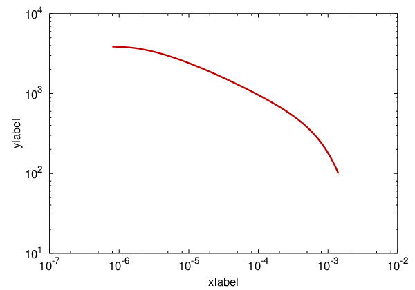
where we have subtracted the pressure induced by the background field $\bar{\varphi}$. Figure 2 shows the cancellation of the pressure contributions for large radii.

As already explained, the cosmon contribution is more extended than the neutrino contribution.

In the cosmological context, the aforementioned conditions are met, at best, approximately and realistic neutrino lumps will not be exactly pressureless. We shall now discuss the three conditions. First, only the total energy-momentum tensor of neutrinos, local cosmon perturbation, and background cosmon is conserved. The background field, however, cannot be attributed to the lump (otherwise, the second condition would not be satisfied). The energy-momentum tensor of the lump, defined to include the neutrinos and the local cosmon perturbation, is thus not exactly conserved due to exchange between the lump and the outside cosmon field. Finally, even for a virialized lump with a fixed number of neutrinos, the energy-momentum tensor is not static. Due to the time evolution of the outside cosmon field, the mass of the neutrinos and therefore the mass of the lump changes.

One may argue that these effects are suppressed by the difference in the relevant time scales for the dynamics of the lump and the cosmological evolution. Indeed, the violations of staticity and energy-momentum conservation are proportional to the time derivative of the cosmon field averaged on length scales much larger than the size of the lump. This is suppressed by the fact that the associated time scale is large as compared to the dynamical time scale of the lump. The effective description of growing neutrino quintessence presented in the next section assumes that the pressure of neutrino lumps approximately vanishes.

Let us introduce a comoving length scale $\lambda$, which is larger than the typical lump sizes but smaller than their typical distances (the mean distance between neighboring lumps is of order $100\,h^{-1}$Mpc). On scales larger than $\lambda$, a lump $l$ at comoving coordinates $\boldsymbol{x}_{l}$ looks effectively point-shaped,

the amplitude $A^{\mu\nu}$ being given by the integrated local energy-momentum tensor of the lump,

We will see in Sec. IV.1 that this indeed reduces to the standard one-particle case

where $M_{l}$ is the lump’s rest mass (consisting of a neutrino and a cosmon contribution) and $u^{\mu}$ is its four-velocity. The Lorentz factor is defined as $\gamma=\sqrt{-g_{00}}\,u^{0}$. In the background metric, we have $\gamma=u^{0}$. The result for $A^{\mu\nu}$ is a consequence of the approximate pressure cancellation discussed in Sec. II.2.

The interactions between the lumps are mediated by the cosmon field $\varphi$. Given that the distances between the lumps are greater than $\lambda$, it suffices to consider the smoothed field (indicated by a hat)

with a suitable window $W_{\lambda}$ of size $\lambda$.

Analogously to the fundamental coupling parameter $\beta$, Eq. (3), we may define the effective coupling by

The effective coupling may depend on the scale $\lambda$ over which the field is averaged. Whereas the fundamental coupling $\beta$ describes the dependence of the microscopic neutrino mass $m_{\nu}$ on the local cosmon field $\varphi$, the effective coupling $\beta_{l}$ measures the mass dependence of the total lump mass $M_{l}$ on the large-scale cosmon value $\hat{\varphi}$. As the fundamental parameter $\beta$ quantifies the force between neutrinos, cf. Eq. (4), the effective parameter $\beta_{l}$ will determine the interactions between lumps.

We next show quantitative results for the distribution of lumps and the effective couplings at $z=1$. For this purpose, we have performed $10$ simulation runs with the method and the parameters of Ref. [8]: fundamental coupling $\beta=-52$, box size $L=600\,h^{-1}$Mpc, but with reduced resolution $N_{\text{cells}}=128^{3}$. The positions of the lumps have been identified as local maxima of the neutrino density field (cf. DENMAX halo finding [15]). A glance at Fig. 1 shows that there is not much ambiguity in identifying lumps.

Once a stable lump has formed, the number of bound neutrinos is approximately fixed (neglecting merging processes). It is thus natural to characterize different lumps by their amount of neutrinos.

We measure the effective couplings $\beta_{l}$ and the lump masses $M_{l}$. The latter include a (dominant) neutrino contribution $M^{(\nu)}_{l}$ and a somewhat smaller cosmon part $M^{(\varphi)}_{l}$. Integration over the comoving lump volume $V_{l}$ yields

with $\rho_{\varphi}=\frac{{\dot{\varphi}}^{2}}{2}+\frac{|\boldsymbol{\nabla}\varphi|^{2}}{2a^{2}}+V(\varphi)$. The Lorentz factor $\gamma$ depends on the velocities of the lumps or particles, respectively. The smoothed field $\hat{\varphi}$ is considered external to the lump and thus subtracted.

Figure 3 shows the abundance of lumps and the distributions of $\beta_{l}$ and $M_{l}$.

The couplings $\beta_{l}$ are measured by numerical differentiation according to Eq. (11). The two lower figures show approximate functional dependences on the neutrino amount with only relatively small statistical fluctuations. The effective coupling is systematically weaker than the fundamental coupling. This becomes more pronounced with increasing neutrino number.

For the averaging scale $\lambda$, we have taken $\lambda=30\,h^{-1}$Mpc. This is clearly smaller than the typical lump distances $\sim 100\,h^{-1}$Mpc but larger than the neutrino concentration of the lumps. Concerning the cosmon field, there remains some ambiguity since we attribute only the cosmon perturbations at scales smaller than $\lambda$ to the lumps. If $\lambda$ is chosen larger, the pressure cancellation and thus the particle approximation are better, cf. Fig. 2, but there may arise overlaps between spatially close lumps.

Within our effective description, the equation of motion of a neutrino lump is derived from the standard one-particle action

with the proper time $\tau$ and the smoothed cosmon field $\hat{\varphi}$ evaluated at the lump trajectory. Along the same lines as for the single neutrino case [8], we arrive at

The left-hand side describes gravity (expansion and gravitational potential), the right-hand side is due to the cosmon-neutrino interaction. The (spatial) term $\beta_{l}\boldsymbol{\nabla}\hat{\varphi}$ is the cosmon-mediated fifth force analogous to Newtonian gravity, cf. Eq. (4). The second contribution on the right-hand side reflects momentum conservation: A lump is accelerated when it moves towards a direction where it loses mass.

In order to use this effective equation of motion, we need to know the smoothed cosmon field $\hat{\varphi}$, the gravitational potential $\Psi$, and the background evolution. In the following, we shall describe how this is achieved.

For the calculation of $\hat{\varphi}$, we recall the coupled Klein-Gordon equation, separated in background and perturbation parts [8],

In Eq. (17) we have neglected the gravitational potential against the cosmon perturbation. The second equation is similar to the gravitational Poisson equation. A natural choice for the cosmon potential $V$ is the exponential potential $V(\varphi)\propto\exp(-\alpha\varphi)$ [16].

Next, we will smooth the perturbation equation (17). For the left-hand side, it is straightforward to show by partial integration that

up to surface terms and neglecting the metric perturbations, $\sqrt{g^{(3)}}\approx a^{3}$. On the right-hand side, we write $\widehat{\delta T_{(\nu)}}=\hat{T}_{(\nu)}-\bar{T}_{(\nu)}$ with the smoothed energy-momentum tensor of neutrinos

We next employ the relation (shown in Sec. IV.2)

Here, the smoothed trace of the energy-momentum tensor of a lump $\hat{T}_{l}$ can be calculated from the effective lump energy-momentum tensor, Eqs. (7) and (9), $T_{l}=T^{\mu\nu}_{l}g_{\mu\nu}$:

With these results, the smoothed perturbation equation eventually reads

Assuming that all neutrinos are bound in lumps, one has

in some cosmological volume $V_{\text{phys}}$.

On scales larger than $\lambda$, the window $W_{\lambda}(\boldsymbol{x}-\boldsymbol{x}_{l})$ in Eq. (22) may be replaced by a point $\propto\delta^{(3)}(\boldsymbol{x}-\boldsymbol{x}_{l})$. For an approximate solution of Eq. (22) at distances larger than $\lambda$ from the sources, we thus use a sum of Yukawa potentials,

with the scalar mass $m_{\varphi}^{2}\equiv V^{\prime\prime}(\bar{\varphi})$. The residual term $\delta\varphi_{\text{res},l}(\boldsymbol{x}-\boldsymbol{x}_{l})$ is needed to cancel the background part $\propto\bar{T}_{(\nu)}$ on the right-hand side and to ensure $\overline{\delta\varphi}=0$ in a simulation volume, similar to $\Psi_{\text{res},l}$ below.

If the lumps are moving rather slowly compared to the speed of light, $\gamma_{l}\approx 1$, the two smoothed metric potentials are equivalent, $\hat{\Phi}\approx\hat{\Psi}$. Numerically, this relation is verified on large scales [8]. Then, we write for the smoothed gravitational potential induced by lumps (with the same approximations as for $\hat{\varphi}$)

The solution is (up to a constant)

where the residual contribution can be given explicitly as $\Psi_{\text{res},l}=M_{l}a^{2}|\boldsymbol{x}-\boldsymbol{x}_{l}|^{2}/V_{\text{phys}}$. The total gravitational potential also includes the matter-induced potential which is calculated as usual. Taking into account relativistic corrections would require the calculation of both potentials, $\hat{\Psi}$ and $\hat{\Phi}$, cf. Ref. [8].

In order to have a full description of the cosmological dynamics, we still need to describe the evolution of the cosmological background, i. e. the Hubble expansion $H$ and the background cosmon $\bar{\varphi}$. The background evolution cannot be calculated without taking into account the backreaction due to the perturbation evolution [17, 8]. Instead, the background and the perturbations have to be evolved simultaneously. In particular, one averages first $\beta{\bar{T}}_{(\nu)}$ as in Eq. (23) and inserts this into the background part of the Klein-Gordon equation (16). In every step, the perturbations enter the background equations via $\beta_{l}$ and $M_{l}$.

The methods developed in the previous sections allow for a considerable simplification of the numerical treatment. Rather than evolving a large number of N-body particles and the fields $\varphi$ and $\Psi$ on a grid, one now merely has to evolve a drastically reduced set of differential equations. This becomes possible as soon as a collection of stable neutrino lumps has formed (at about $z\approx 1$). The preceding cosmological evolution has to be carried out with the comprehensive simulation method of Ref. [8]. Its final state at $z\approx 1$ provides a distribution of lumps at positions $\boldsymbol{x}_{l}$, with neutrino number factions $f_{l}$, rest masses $M_{l}$, and effective couplings $\beta_{l}$. This is the starting point for the simplified scheme.

Section III.2 collects a set of coupled differential equations describing the cosmological evolution. These are the equation of motion (15), the background Klein-Gordon equation (16) with its right-hand side (23) and the usual Friedmann equations. They involve the averaged potentials at the lump positions, i. e. $\{\delta\hat{\varphi}(\boldsymbol{x}_{l})\}$ and $\{\hat{\Psi}(\boldsymbol{x}_{l})\}$ (and their gradients) as given by Eqs. (24) and (26). Finally, the mass change is computed according to $\frac{dM_{l}}{dt}=-\beta_{l}M_{l}\frac{d\hat{\varphi}}{dt}$. All these equations have mutual dependences and can only be solved simultaneously. Cold dark matter, if included, has to be treated with standard N-body techniques. The influence of neutrino lumps on the matter component was studied in [18, 11, 8].

The aforementioned equations are only complete together with functional relations $\beta_{l}(f_{l},\hat{\varphi})$ and $M_{l}(f_{l},\hat{\varphi})$, cf. Fig. 3, known at all times. As a first approach, one may assume a time-independent relation. This is reasonable if the lumps are virialized and hence their inner structure is approximately frozen. We will explore the stability of individual lumps in Sec. V. Furthermore, the dependence on $\hat{\varphi}$ may be neglected if the derivative $\partial\beta/\partial\hat{\varphi}$ or the variation of $\hat{\varphi}$ are sufficiently small.

It is not clear whether $z\approx 1$ is late enough for the virialization process to have sufficiently proceeded. A hint that the cosmological configuration of the neutrinos is stabilizing, however, is given by the evolution of the total neutrino energy $E_{(\nu)}=\int d^{3}x\,\sqrt{g^{(3)}}\,\rho_{\nu}(\boldsymbol{x})\propto\bar{\rho}_{\nu}a^{3}$, shown in Fig. 4.

For $a\gtrsim 0.45$, one observes a transition to a regime with a small constant slope. This would be compatible with a small monotonic change of the large-scale cosmon field and an effective lump mass depending on this field, corresponding to the expectation of approximate mass freezing within neutrino lumps [19]. This may be taken as a hint that the neutrino lump fluid may become a reasonable picture for $a\gtrsim 0.45$.

We now study a single neutrino lump described by its energy-momentum tensor ${T^{\mu}}_{\nu}$ including contributions of the bound neutrinos and the local cosmon field. The lump occupies a volume $V$; its energy-momentum tensor vanishes outside. On scales much larger than the lump size, it is useful to consider the amplitude

We first switch to the rest frame of the lump where we will show ${A^{\mu}}_{\nu}=-M_{l}\,\delta^{\mu}_{0}\,\delta^{0}_{\nu}$. Let us therefor consider the different components separately. Clearly, ${A^{0}}_{0}=-M_{l}$ by definition of the rest mass. $A^{i0}=P^{i}$ is the total momentum and thus vanishes in the rest frame, whereby ${A^{i}}_{0}=0$. It remains to show ${A^{i}}_{j}=0$.

We assume that the lump is approximately static, i. e. its energy-momentum content in a physical volume is conserved,

neglecting the metric perturbations. Together with the energy-momentum conservation equation,

the staticity condition implies $\partial_{i}{T^{i}}_{j}=0$.

It is convenient to define the three-vector $\boldsymbol{v}=({T^{1}}_{j},{T^{2}}_{j},{T^{3}}_{j})$ for a given column $j$. We have just shown $\text{div}\,\boldsymbol{v}=0$. From now on, we choose $i=j=1$ for simplicity. The amplitude ${A^{1}}_{1}$ can then be written as

where $S_{x}$ is the slice of $V$ normal to the $x$ direction. Outside the lump, we extend the area $S_{x}$ to a closed surface. We can equally integrate over this closed surface since there is no contribution outside the lump. We conclude that the integral vanishes since $\text{div}\,\boldsymbol{v}=0$ inside the enclosed volume. This implies ${A^{1}}_{1}=0$. The derivation can equally be done for arbitrary $i$ and $j$, whereby ${A^{i}}_{j}=0$.

In the presence of an external cosmon perturbation $\delta\hat{\varphi}$ sourced by other lumps, the energy-momentum conservation used in Eq. (29) only applies to the full energy-momentum tensor $T^{\mu\nu}_{\text{tot}}$ including the contribution due to $\delta\hat{\varphi}$. Spatial variations of $\hat{\varphi}$ on the scale of the lump are, however, small, such that $\partial_{i}T^{i}_{\text{tot}\,j}\approx\partial_{i}{T^{i}}_{j}=\text{div}\,\boldsymbol{v}$. If the external field $\delta\hat{\varphi}$ varies only slowly, the staticity condition, Eq. (28), applies to the total energy-momentum tensor as well.

The straightforward generalization of the rest-frame result gives the amplitude ${A^{\mu}}_{\nu}=M_{l}\,u^{\mu}u_{\nu}/\gamma$ as anticipated in Sec. III.1. The lump, on scales larger than its size, is described by a standard one-particle energy-momentum tensor

where we have used $u^{0}=dx^{0}/d\tau$ and $\gamma=\sqrt{-g_{00}}\,u^{0}$.

In the effective description, the two dynamic components are the collection of lumps (with the neutrino and a local cosmon contribution) and the cosmon field $\hat{\varphi}$ outside the lumps, which mediates the interaction. This differs from the usual split in the neutrinos $T^{\mu\nu}_{(\nu)}$ and the cosmon $T^{\mu\nu}_{(\varphi)}$ introduced in Sec. II.1. The total energy-momentum content $T^{\mu\nu}_{\text{tot}}$ can thus be expressed in two ways,

The neutrino contribution is completely contained in $T^{\mu\nu}_{\text{lumps}}$. The cosmon field splits into $\varphi=\hat{\varphi}+\delta\varphi_{\text{loc}}$, and the contribution of the local perturbation $\delta\varphi_{\text{loc}}$ is attributed to the energy-momentum tensor of the lumps. The part of the cosmon energy-momentum tensor not depending on the local fluctuation $\delta\varphi_{\text{loc}}$ is

which corresponds to the standard form of a scalar-field energy-momentum tensor.

Only the total energy-momentum tensor is conserved and we want to investigate the energy-momentum flow between the components $T^{\mu\nu}_{(\hat{\varphi})}$ and $T^{\mu\nu}_{\text{lumps}}$. This will yield an effective coupling $\beta_{l}$ between the lumps and $\hat{\varphi}$. The four-divergence of $T^{\mu\nu}_{(\hat{\varphi})}$ is

In order to evaluate the right-hand side, we employ the equation of motion of the full cosmon field $\varphi$ inferred from Eq. (1):

Smoothing this relation at the scale $\lambda$ (cf. Sec. III.1) at linear order in $\delta\varphi_{\text{loc}}$ and inserting into Eq. (35) yields

The right-hand side can be expressed in terms of lump properties by making use of the conservation equation for the total energy-momentum tensor, $\nabla_{\lambda}T^{\mu\lambda}_{(\hat{\varphi})}=-\nabla_{\lambda}T^{\mu\lambda}_{\text{lumps}}$. The part $\nabla_{\lambda}T^{\mu\lambda}_{\text{lumps}}$ can be analyzed in the effective description where lumps are treated as point particles. The equation of motion (15) implies

Comparison with Eq. (37) yields

which is the relation used in Sec. III.2.

The cosmon-mediated fifth force felt by the neutrinos is stronger than but in some respects similar to gravity. The field equation for $\delta\varphi$, Eq. (17), can be compared to the usual gravitational Poisson equation. The cosmon perturbation $\delta\varphi$ thus plays the role of a potential – similar to the gravitational potential – in which a neutrino particle moves. In contrast to the gravitational case, however, the particle changes its mass $m_{\nu}=m_{\nu}(\varphi)$ while moving with velocity $u^{\mu}$ according to

The loss of mass when moving towards a minimum of the potential implies, by momentum conservation, an additional acceleration [8]. Hence, it has to be investigated whether neutrino lumps are unstable, i. e. continuously shrink to smaller sizes until they are stabilized, e. g., by the degeneracy pressure [20].

The cosmon-mediated fifth force, despite the mass variation along a particle trajectory, shares an important property with gravity: the conservation of angular momentum. For example, a single particle moving in a spherically symmetric and static cosmon potential $\varphi(r)$ (in physical coordinates) has the conserved angular momentum

in polar coordinates $(r,\theta)$ and with the Lorentz factor $\gamma$. The equation of motion, written for the radial momentum $p_{r}=\gamma m_{\nu}\dot{r}$, then contains an angular momentum barrier, which prevents the particle from falling into the center. It reads

This is analogous to Newtonian gravity with an angular momentum barrier $\propto L^{2}/r^{3}$ and an inward potential gradient. The only difference is the variation of $m_{\nu}$ (and $\gamma$) along the particle’s trajectory. Since the mass decreases when approaching the center, this even amplifies the angular momentum barrier.

Of course, these results for a test particle in a central potential need not generalize to a distribution of particles forming a lump. There, we define a neutrino angular momentum density $l^{\mu\nu\alpha}_{(\nu)}$ as in special relativity,

which, without the cosmon-neutrino coupling, would satisfy a conservation equation $\nabla_{\alpha}(l^{ij\alpha}_{(\nu)}/a)=0$ due to the conservation equation for $T^{\mu\nu}_{(\nu)}$. Here, derivatives are taken with respect to comoving coordinates. Defining the total spatial neutrino angular momentum

the conservation equation for $l^{ij\alpha}_{(\nu)}$ in the uncoupled case translates to the conservation law

With the coupling, Eq. (2), we instead obtain

and thus

For a spherically symmetric lump and thus cosmon potential $\varphi=\varphi(t,r)$, it is straightforward to show

In this case, the quantity $a^{2}L^{ij}_{(\nu)}$ is indeed conserved. This is related to the fact that a spherically symmetric scalar field does not carry spatial angular momentum,

The conservation of the total angular momentum $a^{2}L^{ij}_{\text{tot}}$ then reduces to the conservation of $a^{2}L^{ij}_{(\nu)}$.

Our considerations hold for an arbitrary isotropic and homogeneous background metric. Thus, $a$ does not need to be the cosmic scale factor but can also describe some local properties of the metric. Fluctuations of the metric around the background metric as well as fluctuations of the cosmon around an averaged field as $\hat{\varphi}$ in Eq. (10) can be added to the neutrino energy-momentum tensor in Eq. (43). The right-hand side of Eq. (48) involves then $\hat{\varphi}$ instead of $\varphi$ and $\beta_{l}$ instead of $\beta$, resulting in a reduction of the change of angular momentum. We conclude that angular momentum conservation is similar to standard gravity. This constitutes a strong hint for a dynamic stabilization of the lump.

We will now study a neutrino lump within a hydrodynamic framework and derive a balance equation for a simple class of lumps. For this purpose, we will employ moments of the neutrino phase-space distribution function $f(t,x^{i},p_{j})$ describing the distribution of particles with comoving position $x^{i}$ and momentum $p_{j}=m_{\nu}u_{j}$. A discussion of stability based on the Tolman-Oppenheimer-Volkoff equation can be found in Ref. [21]. For simplicity, we will restrict ourselves to first-order relativistic corrections in this section. The equations of motion for a neutrino particle under the influence of the fifth force can then be written as

The fully relativistic equation in terms of the four-velocity $u^{\mu}$ is presented in [8].

We will consider the following moments of the phase-space distribution function $f$:

The quantities $n(t,\boldsymbol{x})$, $\boldsymbol{U}(t,\boldsymbol{x})$, and $\sigma_{ij}(t,\boldsymbol{x})$ are interpreted as the number density, the locally averaged peculiar velocity, and the velocity dispersion tensor, respectively. Their evolution equations can be derived from the principle of particle conservation in phase-space, which is expressed by the continuity equation

The whole procedure is similar to the standard case of gravity (cf. Ref. [22]) with the peculiarity of a varying mass $m_{\nu}=m_{\nu}(\varphi)$.

Integrating over the momentum in Eq. (55) yields the zeroth moment

with $\partial_{r_{i}}=a^{-1}\partial/\partial x^{i}$. A static number density profile, $\dot{n}=0$, is realized if the microscopic motion adds locally up to zero, $\boldsymbol{U}=0$. This is the case for a locally isotropic velocity distribution. For this class of lumps, the equation for $\dot{\boldsymbol{U}}$, which follows by taking the first moment of Eq. (55) and using the equations of motion (51), takes a particularly simple form:

with $\sigma\equiv{\sigma^{i}}_{i}/3$.

For a static lump, we demand $\dot{\boldsymbol{U}}=0$ in addition to $\dot{n}=0$. A glance at Eq. (57) shows that this requires a certain balance between the effective pressure $\propto\partial_{r_{j}}\sigma_{ij}$, generated by the microscopic neutrino motion, and the fifth force $\propto\beta\partial_{r_{i}}\varphi$. Assuming spherical symmetry, the balance equation reads

with a prime denoting derivatives with respect to the radial coordinate. Here, we have used $\sigma_{ij}=\sigma\,\delta_{ij}$. Solving this equation together with the (radial) Klein-Gordon equation for the cosmon field yields static lump configurations. These lump configurations differ from the solutions discussed in Ref. [20] since the stabilizing pressure is now provided by the neutrino motion rather than by the degeneracy pressure.

At first sight, it is not clear whether this staticity condition constitutes a stable equilibrium. We perform an exemplary numerical check by simulating a single, isolated lump with the N-body technique [8]. Rather than starting with a static lump configuration by Eq. (58), we use a somewhat smaller velocity dispersion $\sigma$. In the subsequent evolution, the lump shrinks and the neutrino pressure increases. Figure 5 shows how the neutrino profile becomes more concentrated and indeed stabilizes. The simulation evolves the lump in physical time $t$. For convenience, we have translated time intervals $\Delta t$ to scale factor intervals $\Delta a$ by the Hubble parameter at $z=1$.

The pressure cancellation between the contributions of neutrinos and the cosmon perturbations, cf. Sec. II.2, is established during the stabilization process. This is shown in Fig. 6.

Similar to Fig. 2, we observe that the pressure cancellation is only established at rather large distances from the lump. At smaller distances, a residual positive pressure remains.

References

- [1] A. G. Riess et al. (Supernova Search Team), Astron.J. 116, 1009 (1998), arXiv:astro-ph/9805201 [astro-ph]
- [2] S. Perlmutter et al. (Supernova Cosmology Project), Astrophys.J. 517, 565 (1999), arXiv:astro-ph/9812133 [astro-ph]
- [3] M. Doran, G. Robbers, and C. Wetterich, Phys.Rev. D75, 023003 (2007), arXiv:astro-ph/0609814 [astro-ph]
- [4] C. L. Reichardt, R. de Putter, O. Zahn, and Z. Hou, Astrophys.J. 749, L9 (2012), arXiv:1110.5328 [astro-ph.CO]
- [5] L. Amendola, M. Baldi, and C. Wetterich, Phys.Rev. D78, 023015 (2008), arXiv:0706.3064 [astro-ph]
- [6] C. Wetterich, Phys.Lett. B655, 201 (2007), arXiv:0706.4427 [hep-ph]
- [7] D. Mota, V. Pettorino, G. Robbers, and C. Wetterich, Phys.Lett. B663, 160 (2008), arXiv:0802.1515 [astro-ph]
- [8] Y. Ayaita, M. Weber, and C. Wetterich, Phys.Rev. D85, 123010 (2012), arXiv:1112.4762 [astro-ph.CO]
- [9] C. Wetterich, Astron.Astrophys. 301, 321 (1995), arXiv:hep-th/9408025 [hep-th]
- [10] L. Amendola, Phys.Rev. D62, 043511 (2000), arXiv:astro-ph/9908023 [astro-ph]
- [11] M. Baldi, V. Pettorino, L. Amendola, and C. Wetterich, Mon.Not.Roy.Astron.Soc. 418, 214 (2011), arXiv:1106.2161 [astro-ph.CO]
- [12] C. Wetterich, Nucl.Phys. B302, 668 (1988)
- [13] B. Ratra and P. Peebles, Phys.Rev. D37, 3406 (1988)
- [14] N. Wintergerst, V. Pettorino, D. Mota, and C. Wetterich, Phys.Rev. D81, 063525 (2010), arXiv:0910.4985 [astro-ph.CO]
- [15] J. M. Gelb and E. Bertschinger, Astrophys.J. 436, 467 (1994), arXiv:astro-ph/9408028 [astro-ph]
- [16] C. Wetterich, Phys.Rev. D77, 103505 (2008), arXiv:0801.3208 [hep-th]
- [17] V. Pettorino, N. Wintergerst, L. Amendola, and C. Wetterich, Phys.Rev. D82, 123001 (2010), arXiv:1009.2461 [astro-ph.CO]
- [18] N. Brouzakis, V. Pettorino, N. Tetradis, and C. Wetterich, JCAP 1103, 049 (2011), arXiv:1012.5255 [astro-ph.CO]
- [19] N. J. Nunes, L. Schrempp, and C. Wetterich, Phys.Rev. D83, 083523 (2011), arXiv:1102.1664 [astro-ph.CO]
- [20] N. Brouzakis, N. Tetradis, and C. Wetterich, Phys.Lett. B665, 131 (2008), arXiv:0711.2226 [astro-ph]
- [21] A. E. Bernardini and O. Bertolami, Phys.Rev. D80, 123011 (2009), arXiv:0909.1541 [gr-qc]
- [22] F. Bernardeau, S. Colombi, E. Gaztanaga, and R. Scoccimarro, Phys.Rept. 367, 1 (2002), arXiv:astro-ph/0112551 [astro-ph]