In Ref. [12], the amplitudes corresponding to the minimal surfaces in $AdS_{3}$ were analyzed. The classical string equations of motion describing the minimal surfaces were reduced to the $su(2)$ Hitchin system or a generalized sinh-Gordon equation via the Pohlmeyer reduction. The regularized area was divided into several terms, and they were explicitly evaluated for the eight-point amplitudes with the help of the results on the moduli space of a four-dimensional ${\cal N}=2$ supersymmetric theory [24]. The explicit form of the surfaces is not needed in this analysis, as mentioned.

The analysis in Ref. [12] was extended to the minimal surfaces in $AdS_{5}$ in Ref. [13], where the Pohlmeyer reduction led to the $su(4)$ Hitchin system. Interestingly, it was shown there that a non-trivial part of the regularized area for the six-point amplitudes is obtained by solving a set of integral equations, which turn out to be the TBA equations associated with the ${\mathbb{Z}}_{4}$-symmetric two-dimensional integrable model [25]. Following this work, the integral equations for the 10- and 12-cusp minimal surfaces in $AdS_{3}$ were derived in Ref. [1]. The general case of the $\tilde{n}$-cusp minimal surfaces in $AdS_{5}$ was studied in Ref. [14]. For the minimal surfaces in $AdS_{3}$ and $AdS_{4}$, the integral equations obtained there were identified in Ref. [1] with the TBA equations of a two-dimensional integrable model called the homogeneous-sine Gordon (HSG) model [26]. In the rest of this section, we follow the results in Ref. [14].

In order to calculate the $2n$-point amplitudes corresponding to the minimal surfaces in $AdS_{3}$, one first needs to solve the following set of integral equations:

where $s=1,...,n-3$, $\tilde{Y}_{0}=\tilde{Y}_{n-2}=0$, and $\ast$ stands for the convolution, $f\ast g:=\int f(\theta-\theta^{\prime})g(\theta^{\prime})\,d\theta^{\prime}$. The parameter $\theta$ is an auxiliary parameter called the spectral parameter. The complex parameters $m_{s}=|m_{s}|e^{i\varphi_{s}}$ correspond to the shape of the minimal surfaces, which gives the momenta of the external particles through (2.2). By tildes, we denote the shift of the argument of the Y-functions, $Y_{s}(\theta)$, as $\tilde{Y}_{s}(\theta):=Y_{s}(\theta+i\varphi_{s})$. The kernels in the convolution are

where $I_{sr}=\delta_{s,r+1}+\delta_{s,r-1}$ is the incidence matrix of the $A_{n-3}$ algebra. Thus, the “interaction” among the Y-functions are represented by the Dynkin diagram of $A_{n-3}$ (see Fig. 3).

Precisely, the form of (3.1) is valid for $|\varphi_{s}-\varphi_{s\pm 1}|<\pi/2$. Outside this range, it is obtained by continuation, to pick up contributions of the poles in the kernels. Under the condition that $\tilde{Y}_{s}(\theta)$ are analytic for $|\im\theta\,|<\pi/2$, the integral equations are converted into a set of algebraic equations called the Y-system [27]:

where the bracket stands for the shift of the argument,

The Y-functions represent the cross-ratios of the cusp coordinates extended by the spectral parameter. Indeed, one finds that

where $x_{i,j}^{\mu}:=x_{i}^{\mu}-x_{j}^{\mu}$, and the indices for the cusps are labeled modulo $n$. For example, $Y_{1}(-\pi i/2)=x^{+}_{15}x^{+}_{67}/x^{+}_{56}x^{+}_{17}$, $Y_{1}(0)={x^{-}_{15}x^{-}_{67}}/{x^{-}_{56}x^{-}_{17}}$ for $n=7$. Graphically, these cross-ratios are represented by the tetragons inside the $n$-gons formed by $x_{i}^{\pm}$. In Fig. 4, we show an example of $n=7$.

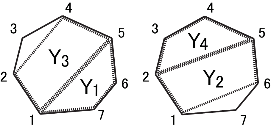
As mentioned above, the equations (3.1) are nothing but the TBA equations of the HSG model. In the context of the two-dimensional integrable model, $m_{s}$ are the (complexified) mass parameters, $\theta$ is the rapidity, and $Y_{s}$ are the exponentials of the pseudo-energies.

Once the Y-functions are obtained by solving the TBA equations (3.1), one can write down the formula of the remainder function, which is defined by the difference between the amplitude and the BDS formula. For the time being, we focus on the case of the $2n$-point amplitudes with $n$ odd. In this case, the formula reads

The overall coupling constant $\sqrt{\lambda}$ has been omitted above. The first term is a constant. The second term, which is given by

comes from period integrals over an auxiliary hyperelliptic curve $y^{2}=p(z)$ with $p(z)$ being a polynomial of degree $n-2$. The third term, which is given by

comes from the difference between a term satisfying the anomalous dual conformal Ward identities and a similar term in the BDS formula. Here, $c_{i,j}^{\pm}$ are the sequential cross-ratios formed by the nearest neighbor distances of $x_{i}^{\pm}$,

Similarly to $Y_{s}$ in Fig. 4, these are graphically represented by polygons inside the $n$-gons formed by $x_{i}^{\pm}$. In Fig. 5, we show an example of $c^{\pm}_{1,6}$ for $n=7$.

The last term is given by the following integral,

Interestingly, this is nothing but the free energy associated with the TBA system (up to a factor). From these expressions, we find that there are two non-trivial parts, $\Delta A_{\rm BDS}$ and $A_{\rm free}$, in expressing the remainder function in terms of the mass parameters $m_{s}$.

Given the formula of the remainder function, what we should do is to solve the TBA equations. They are solved numerically by iterations, to get numbers of $R_{2n}$ for given $m_{s}$. The TBA equations (3.1) are also solved exactly in the limit where all $m_{s}$ approach 0 or $\infty$. The former limit corresponds to the UV limit where the two-dimensional integrable model reduces to a CFT, or to the limit where the corresponding Wilson loops become regular-polygonal. The latter corresponds to the IR limit where the particles in the two-dimensional integrable model become free massive particles, or to soft limits of the SYM theory.

However, the solutions to the TBA system (3.1) have not been fully understood yet. To find the momentum dependence of the remainder function and its structures, one also needs to find the relation between $m_{s}$ and the momenta, since the TBA equations are solved for given $m_{s}$. Here, one may need some analytic data. In addition, interesting analytic results have been obtained at two loops [28, 29, 30, 31]. Taking these into account, it would be worthwhile to explore analytic results at strong coupling besides in the special limits $m_{s}\to 0,\infty$.

This is the subject of the rest of this talk. In particular, we discuss analytic expansions of the remainder function around the UV/CFT limit $m_{s}\to 0$. For later use, here we introduce the mass scale $M$, the length scale $L$ which corresponds to the inverse temperature of the TBA system, the dimensionful mass parameters $M_{s}$ and the relative masses $\tilde{M}_{s}$, so that

In terms of these parameters, the CFT limit we consider is represented as

Since $A_{\rm free}$ is the free energy of the HSG model, it is straightforward to expand it around the CFT limit by using the action (4.1) and CPT. By the standard procedure [8], one has

The first term $c_{n}=(n-2)(n-3)/n$ is the central charge of the coset CFT for $\widehat{su}(n-2)_{2}/[\widehat{u}(1)]^{n-3}$. The second term $f_{n}^{\rm bulk}$ is the bulk term given for $n$ odd by

which cancels with $A_{\rm periods}$ in (3.7). The terms in the summation come from the perturbation by $\Phi$,

where the correlators are connected ones evaluated at the CFT point and we have set $x_{1}=1$. At the lowest order, we have

where

$\gamma(x):=\Gamma(x)/\Gamma(1-x)$, and $G(\tilde{M}_{s})$ is a normalization factor defined through

To determine the dependence on $\tilde{M}_{s}$, one needs to find the precise form of $\Phi(\tilde{M}_{s})$ in terms of the weight 0 adjoint operators. We will come back to this issue later.

Next, let us consider the expansion of $\Delta A_{\rm BDS}$, which is given by the sequential cross-ratios $c_{i,j}^{\pm}$. Interestingly, with the help of graphical representations as in Figs. 4 and 5, one can show that these cross-ratios are directly expressed by the T-functions [32], which are related to the Y-functions as

One then finds for $n$ odd that

Consequently, $\Delta A_{\rm BDS}$ is represented by the T-functions as

where $T_{s}^{[k]}(\theta)$ are evaluated at $\theta=0$. We see that each term in the remainder function (3.6) nicely fits into the language of two-dimensional integrable models: $A_{\rm free}$ is the free energy, and $A_{\rm periods}$ and $\Delta A_{\rm BDS}$ are given by the mass parameters and the T-functions, respectively. Now, we have only to expand $T_{s}$ around the CFT limit.

To expand the T-functions, we use an interesting relation[33, 34, 35] between the T-function and the boundary entropy or the $g$-function [36]. Since the $g$-function is regarded as a boundary contribution to the free energy, one can compute it around the CFT limit by using CPT with boundary [34, 35].

The precise relation between the $g$- and T-functions is obtained by (i) constructing the reflection factors of the HSG model which satisfy the unitarity, the crossing symmetry, and the boundary Yang-Baxter equation, (ii) deriving the integral equations for the $g$-functions associated with the boundaries corresponding to the reflection factors, and (iii) comparing those equations with those for the T-functions. Here, to satisfy the boundary Yang-Baxter equation, the imaginary resonance parameters or the phases of the mass parameters need to be vanishing, as they are in our discussion so far. For details, we refer to Ref. [3].

In expanding $T_{s}$, we then use their quasi-periodicity for $n$ odd,

This follows from the relations (4.10) which are written in the form of the T-system,

with $T_{0}=T_{n-2}=1$. Combining this quasi-periodicity and the structure of the CPT, the T-functions are expanded for real $m_{s}$ and $n$ odd as

with $t_{n-2-s}^{(p,2q)}=(-1)^{p}t_{s}^{(p,2q)}$. The T-system then fixes the lower coefficients as

and $t_{s}^{(1,0)}=t_{s}^{(0,2)}=t_{s}^{(1,2)}=0$. Further using the results on the conformal perturbation of the $g$-function, and translating them into the expansion of the T-functions, we obtain

where $B(a,b)=\Gamma(a)\Gamma(b)/\Gamma(a+b)$. We note that the ratios of the sine functions come from the modular S-matrix of the coset CFT. In relation to the $g$-function, the form of $t_{s}^{(0,0)}$ in (4.16) is also interpreted in this way. From the T-system, one can also show that $t_{s}^{(0,4)}$ are given by $t_{s}^{(2,0)}$ via

Together with (4.17), we see that all $t_{s}^{(2,0)}$ and $t^{(0,4)}_{s}$ are expressed, e.g., by $t_{1}^{(2,0)}\propto\kappa_{n}G(\tilde{M}_{s})$.

From the expansion of $A_{\rm free}$ and the one of $\Delta A_{\rm BDS}$ via those of $T_{s}$, the remainder function is expanded around the CFT limit. After some algebras, we find that

for $n$ odd and real $m_{s}$, where

and

The first term in the expansion $R_{2n}^{(0)}$ gives the remainder function in the CFT limit, or for the regular-polygonal Wilson loops. We also note that $t_{s}^{(3,0)},t_{s}^{(2,2)}$ and $t_{s}^{(4,0)}$ do not appear, and hence $R_{2n}^{(4)}$ is expressed by $t_{1}^{(2,0)}$ or $\kappa_{n}G$.

The absence of $t_{s}^{(3,0)},t_{s}^{(2,2)},t_{s}^{(4,0)}$ in the above expansion is understood as a consequence of the ${\mathbb{Z}}_{2n}$-symmetry, which is the symmetry under the cyclic shift of the cusp points: $k$-th cusp $\to$ $(k+1)$-th cusp or, in terms of the light-cone coordinates,

This is concisely expressed in terms of the Y-functions as [37]

or in terms of the mass parameters as $m_{s}\to m_{s}/i$. Acting with this symmetry twice induces a simple translation $x_{j}^{\pm}\to x_{j+1}^{\pm}$. For general complex $m_{s}$, the expansion of $T_{s}$ in (4.15) is modified so that $t_{s}^{(p,2q)}\cosh(2p\theta/n)\to\frac{1}{2}(t_{s}^{(p,2q)}e^{2p\theta/n}+\bar{t}_{s}^{(p,2q)}e^{-2p\theta/n})$. The shift $\theta\to\theta+\pi i/2$ in (4.23) is thus translated into the phase shift of the coefficients $t_{s}^{(p,2q)},\bar{t}_{s}^{(p,2q)}$. Then, the non-constant invariant combinations under the ${\mathbb{Z}}_{2n}$-symmetry are only $t_{s}^{(2,0)}\bar{t}_{s}^{(2,0)}$ and $t_{s}^{(0,4)}$ up to ${\cal O}(l^{8\over n})$, which explains the terms in the expansion of $R_{2n}$.

So far, we have considered real $m_{s}$ corresponding to the vanishing imaginary resonance parameters. The expansion for complex $m_{s}$ is also obtained so as to maintain this ${\mathbb{Z}}_{2n}$-symmetry: we rewrite the expansion in terms of the ${\mathbb{Z}}_{2n}$-invariant combinations of $t_{s}^{(p,2q)}$, and then continue the real $\tilde{M}_{s}$ in $t_{s}^{(p,2q)}$ to complex $\tilde{M}_{s}$. Up to ${\cal O}(l^{8\over n})$, this procedure reduces to replacing $\kappa_{n}^{2}G^{2}$ for real $m_{s}$ by $\kappa_{n}^{2}G\bar{G}$ for complex $m_{s}$. The ${\mathbb{Z}}_{2n}$-symmetry strongly constrains the structure of the remainder function in this way.

So far, we have focused on the case of $n$ of $2n$ odd. For $n$ even, there are several changes. For example, the remainder function has an extra term $A_{\rm extra}$ in addition to those in (3.6) due to a non-trivial monodromy of an auxiliary variable defined by $dw=\sqrt{p(z)}dz$. The expressions of $A_{\rm periods}$ and $\Delta A_{\rm BDS}$ are also changed. Since $T_{n-2}\neq 1$ generally for $n$ even, the quasi-periodicity of the T-functions is also modified. Due to this, their expansions have extra factors compared with (4.15). The remaining part, which we denote by $\hat{T}_{s}$, however, has the same quasi-periodicity and the form of the expansion as in (4.13) and (4.15), respectively. We refer to Ref. [4] for derails. In any case, since the extra term $A_{\rm extra}$ and the extra factors in $T_{s}$ are irrelevant up to $o(l)$, the expansion of $R_{2n}$ up to ${\cal O}(l^{\frac{8}{n}})$ for $n\geq 10$ is similar to the one for $n$ odd. We then obtain the expansion of the form (4.19) with

for $n\geq 10$. Here, $\hat{A}_{n,s}$ are give by (4.21) with $t^{(p,2q)}_{s}$ replaced by $\hat{t}^{(p,2q)}_{s}$, which are the expansion coefficients of $\hat{T}_{s}$. In the expansion up to this order, the relevant $\hat{t}^{(p,2q)}_{s}$ are however the same as $t^{(p,2q)}_{s}$ and given by (4.16), (4.17) and (4.18).

For $n=6,8$, we have also checked that various modifications in each term in $R_{2n}$ eventually cancel each other, and we are left with the same expression as for $n\geq 10$. The relevant coefficients $\hat{t}_{s}^{(p,2q)}$ are the same as $t_{s}^{(p,2q)}$ and given by (4.16), (4.17) and (4.18) again. The case of $n=4$ is special in that the TBA system becomes trivial. In this case, the integral expression of the remainder function is given in Ref. [12], and is expanded in $l^{2}$ to all orders in Ref. [3].

The expansion for general complex $m_{s}$ is obtained by complexifying $m_{s}$ similarly to the case of $n$ odd.

The expansion so far is given in terms of $|t_{s}^{(2,0)}|^{2}\propto\kappa_{n}^{2}G\bar{G}$. To express the remainder function as a function of the momenta, we need to find the relation between those expansion parameters and the cross-ratios. For this purpose, we first note that the Y-functions have the quasi-periodicity,

for $n$ both odd and even. This follows from the Y-system (3.3). Then, similarly to $T_{s}$, the Y-functions for general complex $m_{s}$ are expanded around the CFT limit as

where $y_{s}^{(0,0)}$ are the solution to the constant Y-system,

From the relations (4.10), we then find that

Inverting this gives

up to the present order, where we have set $t_{s}^{(2,0)}=|t_{s}^{(2,0)}|e^{i\phi_{s}}$, and $\delta Y_{s}^{[k]}$ are the deviations of the cross-ratios from the CFT/regular-polygonal limit, $\delta Y_{s}^{[k]}:=Y_{s}^{[k]}-y_{s}^{(0,0)}$. By using the relations (3.5), these are indeed expressed in terms of the cross-ratios (which depend on each other at this order through (4.28)). The momentum dependence of the remainder function is found by substituting (4.29) into the expansion.

At higher orders, the expansion may not be expressed only by $\kappa_{n}G$. Thus, we need to find the precise form of the perturbing term $\kappa_{n}\Phi$ for given $m_{s}$, i.e., the mass-coupling relation in the HSG model. This is also necessary to make contact with numerics using the TBA system (3.1) for given masses, as well as to find the connection between $m_{s}$ and the cross-ratios/shape of the minimal surfaces.

This is achieved for some cases where the TBA system has only one mass scale. A classification of such cases is given in Ref. [38]. In this subsection, we set $m_{s}$ to be real again. To see this, we first parameterize $\Phi$ as

where $\phi_{l,l^{\prime}}$ are the weight 0 adjoint operators normalized so that $\langle\phi_{l,\bar{l}}(z)\phi_{l^{\prime},\bar{l}^{\prime}}(0)\rangle=\delta_{l,l^{\prime}}\delta_{\bar{l},\bar{l}^{\prime}}|z|^{-4\Delta}$, and $\boldsymbol{\lambda}=\sum_{j=1}^{n-3}\tilde{M}_{j}^{1-\Delta}\boldsymbol{{\hat{\lambda}}}_{j}$. Classically, $\hat{\boldsymbol{\lambda}}_{j}$ are the fundamental weights of $su(n-2)$ [39, 40]. In this parameterization, one has

When the mass parameters are set to be $M_{1}=M,\,M_{2}=\cdots=M_{n-3}=0$, the TBA system reduces to the one for the (RSOS)_n-2 scattering theory [41, 42], which is regarded as a massive integrable deformation of the unitary minimal model ${\cal M}_{n-1,n}$ by the $\phi_{1,3}$ operator. From the result in Ref. [43], we then find that

When only the $k$-th mass parameter is non-vanishing, i.e., $M_{j}=\delta_{jk}M$, the TBA system reduces to the one for an integrable deformation of the coset CFT associated with $\widehat{su}(2)_{k}\oplus\widehat{su}(2)_{n-2-k}/\widehat{su}(2)_{n-2}$ by the $\phi_{1,1,{\rm adj}}$ operator [44]. Using the result in Ref. [45] together with (4.32), we also find that

References

- [1] Y. Hatsuda, K. Ito, K. Sakai and Y. Satoh, JHEP 1004 (2010) 108.
- [2] Y. Hatsuda, K. Ito, K. Sakai and Y. Satoh, JHEP 1009 (2010) 064.
- [3] Y. Hatsuda, K. Ito, K. Sakai and Y. Satoh, JHEP 1104 (2011) 100.
- [4] Y. Hatsuda, K. Ito and Y. Satoh, JHEP 1202 (2012) 003.
- [5] J. A. Minahan and K. Zarembo, JHEP 0303 (2003) 013.
- [6] I. Bena, J. Polchinski and R. Roiban, Phys. Rev. D 69 (2004) 046002.
- [7] N. Beisert, C. Ahn, L. F. Alday, Z. Bajnok, J. M. Drummond, L. Freyhult, N. Gromov and R. A. Janik et al., Lett. Math. Phys. 99 (2012) 3.
- [8] Al. B. Zamolodchikov, Nucl. Phys. B 342 (1990) 695.
- [9] Z. Bajnok, A. Hegedus, R. A. Janik and T. Lukowski, Nucl. Phys. B 827 (2010) 426.
- [10] B. Eden, P. Heslop, G. P. Korchemsky, V. A. Smirnov and E. Sokatchev, Nucl. Phys. B 862 (2012) 123.
- [11] L. F. Alday and J. M. Maldacena, JHEP 0706 (2007) 064.
- [12] L. F. Alday and J. Maldacena, JHEP 0911 (2009) 082.
- [13] L. F. Alday, D. Gaiotto and J. Maldacena, JHEP 1109 (2011) 032.
- [14] L. F. Alday, J. Maldacena, A. Sever and P. Vieira, J. Phys. A 43 (2010) 485401.
- [15] L. F. Alday and R. Roiban, Phys. Rept. 468 (2008) 153.
- [16] J.M. Drummond, G.P. Korchemsky and E. Sokatchev, Nucl. Phys. B 795 (2008) 385.
- [17] Z. Bern, L. J. Dixon and V. A. Smirnov, Phys. Rev. D 72 (2005) 085001.
- [18] L. F. Alday and J. Maldacena, JHEP 0711 (2007) 068.
- [19] J. M. Drummond, J. Henn, G. P. Korchemsky and E. Sokatchev, Nucl. Phys. B 826 (2010) 337.
- [20] Z. Bern, L. J. Dixon, D. A. Kosower, R. Roiban, M. Spradlin, C. Vergu and A. Volovich, Phys. Rev. D 78 (2008) 045007.
- [21] J. M. Drummond, J. Henn, G. P. Korchemsky and E. Sokatchev, Nucl. Phys. B 815 (2009) 142.
- [22] K. Sakai and Y. Satoh, JHEP 0910 (2009) 001.
- [23] K. Sakai and Y. Satoh, JHEP 1003 (2010) 077.
- [24] D. Gaiotto, G. W. Moore and A. Neitzke, Commun. Math. Phys. 299 (2010) 163.
- [25] R. Koberle and J. A. Swieca, Phys. Lett. B 86 (1979) 209.
- [26] C. R. Fernandez-Pousa, M. V. Gallas, T. J. Hollowood, J. L. Miramontes, Nucl. Phys. B 484 (1997) 609.
- [27] Al. B. Zamolodchikov, Phys. Lett. B 253 (1991) 391.
- [28] V. Del Duca, C. Duhr and V. A. Smirnov, JHEP 1005 (2010) 084.
- [29] A. B. Goncharov, M. Spradlin, C. Vergu and A. Volovich, Phys. Rev. Lett. 105 (2010) 151605.
- [30] V. Del Duca, C. Duhr and V. A. Smirnov, JHEP 1009 (2010) 015.
- [31] P. Heslop and V. V. Khoze, JHEP 1011 (2010) 035.
- [32] A. Kuniba, T. Nakanishi, J. Suzuki, J. Phys. A 44 (2011) 103001.
- [33] V. V. Bazhanov, S. L. Lukyanov and A. B. Zamolodchikov, Commun. Math. Phys. 177 (1996) 381.
- [34] P. Dorey, I. Runkel, R. Tateo and G. Watts, Nucl. Phys. B 578 (2000) 85.
- [35] P. Dorey, A. Lishman, C. Rim and R. Tateo, Nucl. Phys. B 744 (2006) 239.
- [36] I. Affleck, A. W. W. Ludwig, Phys. Rev. Lett. 67 (1991) 161.
- [37] D. Gaiotto, J. Maldacena, A. Sever and P. Vieira, JHEP 1103 (2011) 092.
- [38] F. Ravanini, R. Tateo, A. Valleriani, Int. J. Mod. Phys. A 8 (1993) 1707.
- [39] C. R. Fernandez-Pousa and J. L. Miramontes, Nucl. Phys. B 518 (1998) 745.
- [40] P. Dorey and J. L. Miramontes, Nucl. Phys. B 697 (2004) 405.
- [41] Al. B. Zamolodchikov, Nucl. Phys. B 358 (1991) 497.
- [42] H. Itoyama, P. Moxhay, Phys. Rev. Lett. 65 (1990) 2102.
- [43] Al. B. Zamolodchikov, Int. J. Mod. Phys. A 10 (1995) 1125.
- [44] Al. B. Zamolodchikov, Nucl. Phys. B 366 (1991) 122.
- [45] V. A. Fateev, Phys. Lett. B 324 (1994) 45.
- [46] T. R. Klassen and E. Melzer, Nucl. Phys. B 350 (1991) 635.
- [47] P. Dorey, D. Fioravanti, C. Rim and R. Tateo, Nucl. Phys. B 696 (2004) 445.
- [48] A. Brandhuber, P. Heslop, V. V. Khoze and G. Travaglini, JHEP 1001 (2010) 050.
- [49] P. Dorey, C. Dunning and R. Tateo, J. Phys. A 40 (2007) R205.