An Independent Measurement of the Incidence of MgII Absorbers along Gamma-Ray Burst Sightlines: the End of the Mystery?
Abstract
In 2006, Prochter et al. reported a statistically significant enhancement of very strong Mg II absorption systems intervening the sightlines to gamma-ray bursts (GRBs) relative to the incidence of such absorption along quasar sightlines. This counterintuitive result, has inspired a diverse set of astrophysical explanations (e.g. dust, gravitational lensing) but none of these has obviously resolved the puzzle. Using the largest set of GRB afterglow spectra available, we reexamine the purported enhancement. In an independent sample of GRB spectra with a survey path 3 times larger than Prochter et al., we measure the incidence per unit redshift of Å rest-frame equivalent width Mg II absorbers at to be . This is fully consistent with current estimates for the incidence of such absorbers along quasar sightlines. Therefore, we do not confirm the original enhancement and suggest those results suffered from a statistical fluke. Signatures of the original result do remain in our full sample ( shows an enhancement over ), but the statistical significance now lies at c.l. Restricting our analysis to the subset of high-resolution spectra of GRB afterglows (which overlaps substantially with Prochter et al.), we still reproduce a statistically significant enhancement of Mg II absorption. The reason for this excess, if real, is still unclear since there is no connection between the rapid afterglow follow-up process with echelle (or echellette) spectrographs and the detectability of strong Mg II doublets. Only a larger sample of such high-resolution data will shed some light on this matter.
Keywords:
gamma-ray: burst - techniques: spectroscopic - quasars: absorption linesI Introduction
In the last decade, the study of the inter-galactic (IGM) and circum-galactic medium (CGM) has received a great boost thanks to large spectroscopic surveys of distant quasars, in particular the dataset provided by the Sloan Digital Sky Surveys [82]. These objects randomly sample thousands of lines of sight and, being bright background sources of light, probe gas and matter located in foreground objects.
One of the most commonly surveyed set of transitions in quasar spectra is the Mg II doublet at Å. Its common detection stems from the large rest wavelength (which makes them easily detectable by most optical spectrographs when the absorber is located at redshift ), the relatively high abundance of Mg, and the strength of this resonance-line doublet. The Mg II systems are frequently classified in terms of the rest-frame equivalent width, , of the bluer component as “weak” ( Å), “strong” ( Å), and “very strong” [66, Å, like in]. For simplicity, throughout the paper we will refer to this last category as “strong”, since it is the only one pertinent to this work. Mg II doublet lines have been surveyed extensively from in the optical passband and now to with near-IR spectroscopy [72, 54, 62, 64, 70, 83, e.g.]. The results indicate that while the weak and strong absorbers incidence show small if any evolution with redshift, the very strong Mg ii absorbers present an increasing trend up to before declining at higher redshift [62, 46]. This evolution rather closely tracks the cosmic star formation history [62, 83], suggesting that some systems may be causally connected to on-going star formation [49, 46], although, accurate analysis of the SDSS survey needs to be carefully taken into account in order to avoid technical biases [45].
For several decades now, strong Mg II absorption has been associated with gas in and around galaxies. Early work identified a small sample of galaxies at modest impact parameters ( kpc) to quasars exhibiting strong Mg II absorption [4, 43, 71] , although no significant trend has been found for a population of Luminous Red Galaxies [e.g. 8, and references therein].
These observations motivate the association of Mg II gas with the outer disk and/or CGM of these galaxies. Several QSOs line of sights presenting Mg ii absorbers have been explored in order to probe the extent and the baryon content around low- galaxies [37, 15, and reference therein], as well as a diagnostic of the inner part of these galaxies’ interstellar medium [7]. Also, a stack analysis was performed by [84] using light profiles (from associated galaxies) of quasars exhibiting strong Mg II absorption in the SDSS. With their image-stacking technique they studied the cross-correlation between the Mg ii gas and the galaxy light from 10 to 200 kpc, finding that strong Mg ii absorbers may be explained by models that include metal-enriched outflows from star-forming/bursting galaxies. Most recently, several attempts to trace the covering fraction and nature of Mg II absorption by targeting known galaxies with coincident background quasars have been performed [3, 13, 81]. Their results indicate the mean covering fraction increases from for Å to for Å, confirming that extended Mg ii absorbing haloes are a common feature around normal galaxies. Finally, it has been found that “strong” absorbers are often associated with nearby (within 75 kpc) galaxies along the line of sight [38, 53, 13].
The survey and analysis of Mg II gas is no longer limited to quasar spectroscopy. For example, researchers have now used distant galaxies to probe foreground galaxies enabling searches at very small impact parameter [67] and statistical ‘maps’ of the absorption correlated with the foreground galaxy orientation [6]. Similarly, Gamma-ray Bursts (GRBs), with their extraordinarily bright optical afterglows provide not only direct information on their host galaxies, but also trace matter intercepting their lines of sight [50].
The advantage of using GRBs as background sources is twofold: first, they can be observed up to very high redshifts [40, 73, 68, 21], which allows one to explore a larger redshift path length, and second, their discovery is largely unbiased with respect to intrinsic properties of their hosts (extinction, luminosity or mass). When a GRB fades away, they leave the line of sights clear for future deep observations in order to search for the Mg II counterparts [80, 36, 69, 12]. One of the first attempt to identify the nature of three absorbers along GRB 060418 was performed by [56], which identified the absorbers to be galaxies at very small impact parameter from the GRB location ( kpc). Deep imaging of several other fields have confirmed these early findings [14]. On the other hand, the number of GRBs discovered and spectroscopically observed is several orders of magnitude less then the number of quasars available in large optical surveys (e.g. SDSS DR8). This difference has been reduced, however, with the success of the Swift satellite providing the discovery and follow-up of several hundred GRBs [29, 30].
Shortly after the launch of Swift in November 2004, a survey of Mg II absorption in GRB afterglow spectroscopy was performed for an early sample of Swift bursts and a heterogeneous sample of pre-existing GRB spectra [63, P06 hereafter]. The authors revealed an extremely puzzling result: the incidence of strong (Å) intervening Mg II absorbers was about 4 times higher along GRB sightlines than quasar sightlines. Despite the small sample size, the statistical significance of their dataset was high: the null hypothesis that GRBs and quasar spectra would show identical incidences of strong, foreground Mg II absorption was ruled out at confidence.
The authors proposed several hypotheses that might explain the difference, which have since been studied in greater detail: 1) a possible intrinsic origin of these absorbers associated near the GRBs themselves [20, 5]; 2) a significant dust bias along QSO lines of sight [48, 58, 9]; 3) a geometric effect difference due to the sizes of the emitting regions between GRBs and QSOs [27, 58, 44] ; 4) a gravitational lensing effect [76, 57, 65]. Subsequent work has ruled out several of these possibilities and none appears to be sufficient on its own to explain the observations. After seven years of the Swift mission and more than two hundred GRBs with spectroscopic confirmations, this mystery remains.
It is important to emphasize that the original P06 work, and even the studies that have followed, have relied on a small sample of GRB afterglow spectra. Even the largest analysis to date analyzed only 26 line of sights (finding 22 absorbers), for a total redshift path of [76]. Furthermore, no study has analyzed a completely independent set of GRB sightlines from the P06 analysis.
In this paper, we use data obtained primarily during the Swift era by several facilities, to obtain the most complete sample of GRB afterglow spectra and the largest redshift pathlength available to date. From this parent sample, we are able to construct sub-samples which are entirely independent from the original work of P06. Similarly, we can study possible instrumental biases (e.g. spectral resolution) which may affect the final results.
The paper is structured as follow: in §II we describe our dataset and the data analysis procedure, while in §III we present our procedure for defining the redshift path density per GRB sightline. §IV describes the search methodology to identify possible Mg ii systems along every line of sight, with distinction between different datasets (e.g. high-resolution vs. low-resolution, strong vs weak Mg ii equivalent width). Finally, in Section §V and §VI we present our findings, including interesting sub-samples results, and we summarize them in light of possible steps forward into understanding this puzzling phenomenon. All the quoted errors, unless otherwise stated, are considered at 1- confidence level.
II Data Selection
The acquisition of an optical spectrum from a given GRB afterglow is a complex and unrepeatable process. During the Swift era, the timelapse between the discovery of the gamma-ray emission (by the Swift/BAT instrument) and the afterglow localization (by XRT and/or UVOT on-board the spacecraft) is generally less than a few minutes, with some exceptions due to observability constraints which delay the satellite to slew towards the BAT position (e.g., due to the small angular separation between the GRB and the Moon or the Sun).
The on-board localization has an accuracy between several arcminutes (BAT only) to subarcseconds (UVOT). The immediate transmission to the ground of all the Swift-acquired data via the Gamma-Ray Burst Network [2] allows rapid (seconds to hours) follow-up with ground-based optical/IR telescopes.
In most of the cases presented in this paper, rapid follow-up spectroscopic observations were triggered as soon as an X-ray counterpart position was delivered (XRT identified more than 98% of the BAT GRBs). Before the actual trigger is sent to the opportune telescope, we check the current telescope/camera set-up available, the visibility window at the telescope site, and weather conditions. A finding chart is usually provided to the telescope operator, using archival images (usually SDSS or USNO catalogues), which also helps to identify the afterglow. Once the trigger is sent to the telescope, usually via Target of Opportunity (ToO) programs, a long acquisition image of the field is acquired. In the eventuality that a “new” source has been found inside the XRT error circle (by comparison with the finding chart), a spectroscopic sequence is executed.
In other cases, especially for high- bursts, robotic, real-time follow-up by different facilities have provided similarly accurate identification within the first hour, using redder filters than the ones available on Swift/UVOT [32, 77, e.g. the GROND and RAPTOR instruments,]. Thanks to the prompt responses, different groups have been able to obtain spectroscopic observations of the optical afterglow when it was bright enough to detect absorption lines, which generally yields a definitive estimate of the GRB redshift. For this purpose, the identification of fine-structure lines represents a secure determination of the GRBs host galaxies and the GRB circumstellar environment [60]. Other secure identification is the presence of a Damped Lyman- system, which also has been signature of a typical high- GRB host galaxy environment. Whenever these features are not present, we assume that the higher redshift system of absorption features from several ionized transitions corresponds to the GRB redshift, but obviously does not guarantee that these features do not rise, instead, in foreground objects along the GRB line of sight [55, see for example GRB 071003,].
For GRBs that occurred before the launch of the Swift satellite a similar procedure was followed: the gamma-ray identification was made by high-energy facilities in orbit (BATSE, HETE-2 spacecrafts), while X-ray observations were due to slower response missions (like Beppo-SAX), which required several hours to repoint. This inevitable delay propagated often to a late follow-up observation, which, in few cases, led to a spectroscopic sequence to executed.
For our parent sample, we set out to obtain the optical afterglow spectra for all GRBs with reported redshifts, restricted as follows. Because of our interest in detecting Mg ii lines, and because most spectrographs have wavelength coverage beginning at Å (or poor UV sensitivity), we require the Mg ii doublet rest-frame wavelength to be redshifted beyond this limit. This leads us to include all the publicly available spectra obtained from GRBs with redshift higher than .
The spectra analyzed in this paper were obtained with facilities across the world, including the Gemini Observatory, Keck Observatory, and Very Large Telescope. Many of these data were obtained by our respective research teams, although several tens were taken from public data archives or were kindly contributed by members of the community. Table 1 lists all of the sightlines with reported GRB redshifts where we were able to retrieve a spectrum. The last column lists the literature references for GRB afterglow spectra that have been previously published.
A small sample of seven GRB spectra, as mentioned in §I, was obtained during the pre-Swift era: these GRBs were discovered by non-GRB dedicated missions, like the Interplanetary Network (GRB 000926), Beppo-SAX (GRB 010222) and HETE-2 (GRB 020813,GRB 021004,GRB 030226,GRB 030323,GRB 030429), and followed from the ground several hours (if not days) after the events were discovered. Neverthless, these data have sufficiently high quality to be included in our work.
Our large dataset consists of a total of 118 GRB afterglows observed by different facilities and instruments, including the Gemini telescopes with the GMOS instruments (46 spectra), the Very Large Telescope equipped with FORS1, FORS2, UVES, and the X-Shooter spectrographs (55), the North Optical Telescope (NOT) with the ALFOSC camera (6), the Keck telescopes with the HIRES,LRIS and ESI instruments (13), and the Magellan Clay telescope with the MagE spectrograph (1). Finally, we also include two spectra obtained by the KAST spectrograph mounted on the 3-m Shane Telescope at Lick Observatory and several from the Magellan and the Telescopio Nazionale Galileo (TNG). The spectral resolution of these data ranges from 450 km/sec (or Å , NOT/ALFOSC) to 7 km/sec (Å, HIRES/UVES). This large variety of data give us the opportunity to test different subsamples drawn from the overall 118 GRBs. All the data presented are part of a public repository of GRB spectra11 1 http://grbspecdb.ucolick.org/.
The VLT sample has been obtained with a specific set of observational criteria, making the best use of the different instruments available and the technical improvement for ToO observations, like the Rapid Response Mode (RRM), which allows the observer to execute the required observation remotely and without a major intervention by the telescope operators [28, see].
Most of the FORS1/2 data are part of the catalog presented in [28] and [22], while most of the high-resolution ones (HIRES, ESI, UVES) were already published in single-GRB papers or as part of [76]. A large fraction of the Gemini spectra are presented here for the first time, and are the result of our group’s follow-up efforts over the last 7 years [18, see also ]. We encourage the readers to refer to the reference in the last column in Table 1 for the data reduction procedures and the original published papers. In the following sections we will briefly review the reduction procedure for the Gemini and the X-Shooter data.
II.1 Gemini sample
These datasets are part of several follow-up programs for which Target of Opportunity time was awarded between 2005 and 2011. All the data included were obtained with the Gemini Multi-object spectrographs [33, GMOS;]. The typical observation sequence consists of two spectra in two dithered positions along the slit (usually 1″ wide) in order to facilitate sky-line subtraction. Immediately before or after the science frames, a ThAr lamp is observed and a flat field is obtained in order to allow data reduction “on-the fly”.
We used the GEMINI/GMOS data analysis packages under the IRAF22 2 IRAF is distributed by the National Optical Astronomy Observatory, which is operated by the Association for Research in Astronomy, Inc., under cooperative agreement with the National Science Foundation. environment in order to perform the basic reduction, flat fielding and wavelength calibration. Cosmic rays were identified and replaced by a median of the surrounding pixels which were not flagged as bad pixels. For this purpose we used the lacos_spec tool [75]. Finally, one frame was subtracted from the other to remove the strongest skylines. This procedure provides good results at Å, but leaves significant residuals in the reddest portion of the spectra where the GMOS spectrographs suffer substantial CCD-fringing. Therefore, the extracted error arrays associated with the Gemini-GMOS data reflect these higher-noise patterns at longer wavelengths.
One dimensional spectra were then extracted using the IRAF APALL tool and coadded weighting each spectrum by the inverse of its variance spectrum in order to increase the of the final result. The APALL package also produces a 1-d array with the poissonian statistical error and the 1-d sky background (estimated in regions selected far from the object trace, so to avoid any spurious contamination). These last two arrays have been summed in quadrature to obtain the final error array per pixel. In some cases we assess the quality of the extracted error array with the estimated RMS of the data-array and modified the latter in order to fully account for the poissonian fluctuations in the actual data. Finally, using the splot routine we estimated signal-to-noise over the whole wavelength range (also reported in Table 1).
II.2 X-Shooter data
Data for GRB 090926A and GRB 100418A, were obtained via the ESO Archive33 3 Based on observations made with ESO Telescopes at the La Silla Paranal Observatory under programs ID 60.A-9427(A) and ID 085.A-0009(B) and reduced with version 1.3.7 of the X-Shooter pipeline [31] in physical mode. The spectra in the UVB and VIS arms were used for the redshift pathlength estimate as well as the Mg ii search. We do not use NIR arm due to the high level of contamination from skylines in the infrared. Furthermore, the infrared sample of QSO spectra, largely obtained by [46], are still small compared to the large compilation from SDSS.
II.3 Subsamples
The set of spectra listed in Table 1 comprises our full sample for analysis which we refer to as Sample F. This sample maximizes the survey path for Mg II absorption along GRB sightlines. From this parent sample, we consider several subsamples for the same analysis. Most important is the independent subsample (Sample I) which ignores all of the data analyzed in the original paper of P06. We focus first and foremost on this subsample to perform a complementary study. In addition, we consider two other subsamples which cut the data according to spectral resolution: we combined all the high-resolution spectra, obtained with echelle or echellette spectrographs (ESI, HIRES, MagE and UVES) in Sample H and, all other data in Sample L. These are summarized in Table 2.
III Survey Path
The starting point of a survey for intervening absorption-line systems is to estimate the redshift path density . This function expresses, as a function of redshift, the number of unique sightlines for which an absorption line could be detected in the survey to a limiting equivalent width. In practice, one determines for each spectrum those regions that have sufficient S/N and are free of strong blending by terrestial or intrinsic gas. These specific windows define redshift intervals , , for the th quasar (or GRB) where within each window and zero otherwise. By integrating across the full spectrum, one recovers the redshift path covered by the source.
To properly determine for each sightline, several issues must be considered to minimize systematic effects that could bias the search. First, we exclude from the search the wavelengths (or the redshift ranges) that fall in the atmospheric telluric bands, which heavily absorb the afterglow flux, rendering it very difficult to identify any features (intrinsic to the GRB, or QSO, host or intervening). Since some of our spectra extend towards the near-IR regime, we also consider atmospheric absorption at these wavelengths. A complete list of the excluded regions is presented in Table 3.
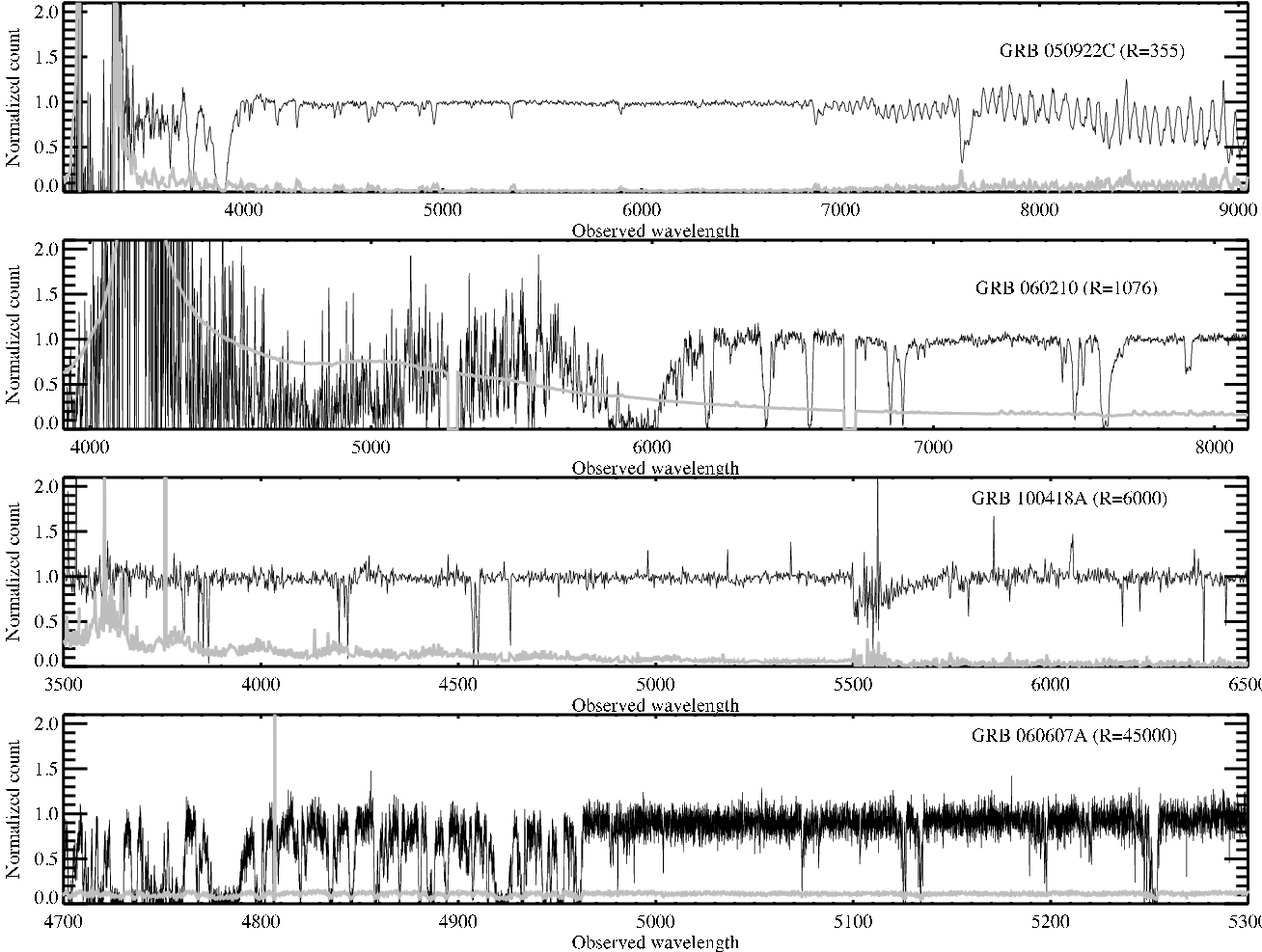
Second, GRB afterglow spectra exhibit strong absorption lines belonging to ionic species located in the progenitor environment and up to tens kpc along the line of sight. The number of detected host features varies depending on the brightness of the afterglow, the properties of the host galaxy, the signal-to-noise and the resolution of the spectrograph (see Figure 1). [16] created a high- composite spectrum using 66 afterglow spectra obtained with low and mid-resolution spectrographs. Strong absorption lines were identified as well as weak ones previously undetected in the individual spectra. Since most of these lines are common in GRB host galaxies we compile a sublist of these absorption features to be excluded in our redshift pathlength calculation. We included also some of the most common fine-structure transitions. To be more conservative, a region equivalent to one half-resolution element both blueward and redward of the observed central wavelength of the considered transition (as set by the redshift of the host galaxy) has had set to zero. In the cases of high-resolution spectra, the minimum size of the masked region is 200 km/s. A complete list of these features is also presented in Table 3.
Finally, for some of the spectrographs (e.g. UVES, GMOS), the spectral coverage is non-contiguous due to gaps between detector chips and/or the use of multiple cameras. Regions without data were simply masked in the evaluation. In several cases, regions beyond Å were heavily effected by fringing, even after correcting for it in the data processing. We opted for a visual inspection of the data and decided on a case-by-case which regions needed to be excluded for the search.
As an example, in Figure 2 we present the Gemini/GMOS spectrum of GRB 060210, where all of the masked regions are indicated. It is clear from Figure 2 that the maximum redshift, , allowed for our intervening Mg ii search is dictated by the host galaxy redshift, in particular, we begun our search starting 1500 km s-1 blueward the corresponding Mg ii feature (or ). Also, the minimum, , is indicated either by the bluest wavelength covered by the spectrograph or, as in the case of GRB 060210, by the presence of the Ly feature (at rest-frame Å) such that , where (or equivalently km s-1 redward the Ly feature). We do not extend the search for intervening Mg II into the Ly forest and we avoid the (typically) very strong damped Ly absorption profile of the GRB host galaxy.
Once these regions have been excluded we determined the equivalent width limit per pixel, using the variance spectrum associated to each object (shown as red in Figure 2), considering a simple gaussian profile of , where is the resolution element. At each unmasked pixel in the spectrum, we query whether the equivalent width limit exceeds a given rest-frame survey limit for Mg II 2796 (e.g. 1Å). If the limit is satisfied, we query whether the corresponding Mg II 2803 line lies in an unmasked region. If both of these criteria are satisfied, for the redshift interval covered by that pixel otherwise we set . This generally leads to a series of discontinuous redshift intervals for the Mg II survey, as listed in Table 4.
Figure 3 presents the total redshift path density for Sample F and Sample I, which represents the number of GRB sight-lines available for our Mg ii search as a function of redshift. These are shown for a limiting rest-frame equivalent width of 1Å at 5 confidence. It is immediately clear from this figure that we accurately excluded from our analysis the telluric lines regions (i.e. at and ). Also, the analysis is mainly performed where we have the majority of the searchable path, in the interval range, due to the larger statistical sample from the GRB and the QSO samples.
The total of the survey crudely expresses its statistical power. This may be calculated by simply summing the values for each source. For the full sample (F), a redshift pathlength of for the 1Å equivalent width limit. For the independent sample (I), we find . The latter represents a 4 times larger survey sample than P06.
IV Identifying and measuring intervening Mg ii absorbers
We described in the previous section the construction of the redshift path density which defines, for each spectrum, the regions where an intervening Mg ii doublet may be detected at significance. Independent of this calculation, we have searched each sightline for the presence of Mg ii absorbers.
Using the algorithm for optimal extraction [34], we constructed an equivalent width spectrum by convolving the normalized data with a Gaussian profile with width set by the resolution of the spectrograph and weighting the flux at each wavelength by the associated variance. From this array, we determined every feature satisfying a detection threshold via an automatic procedure similar to the C iv doublet search performed in [17]. We considered each line as a possible Mg ii absorber, and confirmed this association through the presence of a proper Mg ii doublet (both in velocity separation and relative ). Finally, we inspected every candidate identified by this procedure visually, confirming the presence of a genuine doublet with the additional identification of other common features (e.g. Mg i Fe ii). We also accurately measured the equivalent widths of the doublet components via line profile fitting (see Table 5). As sanity check, each GRB sightline was also manually inspected by the lead authors in search of Mg ii doublets that might be missed by the automatic screening process. We found two doublets in addition to the candidates automatically identified which may be Mg ii features (see §IV.1 for our completeness analysis). Also, we found some doublets which were misidentified as Mg ii doublets: in reality these features were host galaxy fine-structure transitions or other metal lines belonging to other intervening systems (e.g. GRB 061121). We estimated that our total redshift pathlength would be decreased of a factor of if we would have masked also these features, therefore we prefer not to exclude these spectral regions to preserve a maximum searchable path. Again, our visual inspection prevent these features to be accounted in our Mg ii search.
Table 5 lists the Mg ii systems that have been discovered, and Figures 10a–10m show the line-profiles of all the strong Mg ii systems in combination, when available, with other metal features. The values for the Mg ii doublet were estimated by fitting the line-profiles with Gaussian profiles or in the case of line-black saturated transitions (e.g. high resolution data) by pixel summation. We estimated the uncertainty in our values by summing the pixel-by-pixel variance in quadrature.
IV.1 Completeness estimate
It is important to note that the sample under consideration has been obtained by a large variety of facilities and, also, GRBs have been observed at different epochs (meaning at different afterglow brightness) as well as with different atmospheric conditions. Therefore, it is worthwhile evaluating our completeness in finding very strong Mg ii absorbers at the considered confidence level. To assess our completeness we inserted mock Mg ii features into our spectra (taking into account the S/N and the resolution of the original spectra) and then we re-process these new datasets via our automatic procedure. The injected features, in a number which is drawn by a poisson distribution centered on the expected number of absorbers () for the GRB sample, have random equivalent widths between 0.05 to 5Å and a maximum number of seven sub-components, each with a range of doppler parameters km/s. These features were inserted between and as defined in Sec.III per each GRB. We repeated this process 50 times per sightline for a total of 5250 iterations. We compared the number of injected strong features (Å) that should be automatically identified because they were located in regions of the spectra were , (accordingly to Sec. III) with the actual recovered list: we conclude that of the systems were correctly identified and detected as genuine strong Mg ii doublets. Figure 4 shows the result of our completeness test: on the top panel we show the total number of absorbers correctly identified (black histogram) and not (in red) depending on the instrument resolution. It is clear that the lowest-resolution spectra (e.g. the V300 grating with the FORS1 spectrograph) have a low completeness level using our automated search but that the other spectra give excellent results. For the missed absorbers in the lowest-resolution data, we find that these doublets are usually self-blended (resembling a single broad line) or they are blended with the profile wings of other lines (intervening systems metal lines or host galaxy features) preventing the automatic identification of both doublet components.
We examined again our original sample and we confidently retrieved only two such cases: GRB 090812 and a possible absorber at and GRB 070110 with a possible doublet at . Nevertheless, including such features, which were not automatically recovered, does not effect our conclusions.
In the bottom panel of Figure 4 we present our cumulative completeness level with increasing resolution. Again, as noticed previously, we reach level around the resolution of the Gemini-GMOS instrument (R400 grating, ), whose spectra provide the best combination of Signal-to-Noise ratio and resolving power to properly identify the population of strong Mg ii absorbers characterizing the GRB intervening system population.
V Results
V.1 Incidence
Combining the results from the previous two sections, we may estimate the incidence of Mg ii absorption per unit redshift (also referred to as or ). The standard estimator for to a limiting is the observed ratio of the number of absorbers discovered, , having in a given redshift interval to the total redshift pathlength searched, , in that redshift interval
| (1) |
with
| (2) |
Figure 5 presents our estimates for Å Mg ii absorbers, for Sample I and Sample F restricted between and 2. The error estimates assume Poisson statistics for and correspond to 68% confidence. The values for the GRB sightlines have roughly constant value with redshift at and for Sample I and Sample F respectively.
For comparison, we display a fit to the measured values for Å Mg ii absorbers discovered along the thousands of quasar sightlines drawn from the SDSS [83]. These spectra have been chosen to have , so to assure a high confident statistical sample of Mg ii.
This quasar sample was searched for Mg ii absorbers at wavelengths redward of the strong C iv quasar line (Å) and blueward of the reliable response of the Sloan fibers up to the quasar’s Mg II emission line.
From Figure 5 it is evident that while the Sample I follows the expected distribution derived from the QSO analysis, Sample F still presents a modest excess of absorbers. In the case of Sample F, for instance, and the number of absorbers identified is (). Overall the , a factor greater than the expected quasar density of absorbers (). Considering the independent sample, which as mentioned in §II.3 excludes all the lines of sight in PO6, we obtain . Following the same analysis, similar results are evident using the high-resolution and the low-resolution samples (Sample H and Sample L): in these cases we identify an overabundance of strong Mg ii absorbers in the high-resolution sample, leading to a , a factor 2.6 larger then the expected (). We summarize our analysis in Table 2.
Figure 6 shows the cumulative distribution of Mg ii absorbers detected from GRB Sample F and Sample I, together with the quasar estimates. We may compare these results against the predicted cumulative distribution functions for a QSO survey with identical search path to the GRB analysis by simply convolving the GRB with :
| (3) |
It is evident that the full Sample F exhibits a modest excess of , but that the independent Sample I shows no excess. The new results for Sample I do not confirm earlier works which reported an excess of strong Mg II absorption along GRB sightlines.
V.2 Monte Carlo Analysis
To assess the significance of these results, in particular the observed excess for Sample F, we perform a Monte Carlo analysis as follows. First, we selected a set of 12700 SDSS quasars from [83] that have a continuous redshift path density from to , where is the greater of 0.4 and and . This is the brighter subset of quasars in the SDSS with correspondingly higher S/N spectra. Restricting our Monte Carlo analysis to this QSO sample facilitates the generation of random samples with a survey path identical to the GRB analysis.
For GRBs with , an SDSS QSO matched in redshift will cover the survey path of the GRB analysis. For a given GRB, we selected all quasars close in redshift space to (usually in the range there were always at least 50 such quasars). In each Monte Carlo realization we randomly picked one and by construction adopted the from the reference GRB spectrum. We then identified the total number of absorbers discovered by [83] along the lines of sight of these quasars and recorded those that satisfy the Å limit and have .
For , the Mg II survey performed by [83] using the SDSS quasars does not extend as low in redshift as our GRB analysis because those authors truncated the search bluer then the C IV emission peak. As a result, we considered two approaches to handling this difference. The cleanest approach is to artificially truncate the GRB analysis at the same starting redshift as the quasars, i.e.,
| (4) |
The other ‘hybrid’ approach, which maximizes the survey path of this Monte Carlo comparison, is to introduce a second random quasar (with ) to cover the redshift path at in the GRB spectrum. In these cases, the minimum quasar redshift is . Finally, for very high-redshift GRBs () the second quasar has to be chosen such that and , which allows us to select at least 50 QSOs covering the desired redshift path coverage.
We ran ten thousand Monte Carlo iterations using both approaches and we recorded for each iteration the number of Mg II absorbers recovered. We performed this analysis for each of the GRB samples. Figure 7 presents our outcomes using the hybrid approach, though no relevant differences are present using the truncated redshift path.
The results indicate that the incidence of Mg II absorbers detected in our independent Sample I are consistent with the results along quasar sightlines. In fact, we recovered a slightly greater number of absorbers on average along the quasar sightlines. Furthermore, the analysis shows that there is no statistically significant discrepancy between the expected total number of absorbers along the QSOs and the full parent GRB sample (Sample F). In of our simulated quasar lines of sight, we observed a number of absorbers equal to or larger than the Sample F (corresponding to a significance). Only in the case of the high-resolution sub-sample, Sample H is there a statistically significant excess. This sample, however, is dominated by the sightlines analyzed in previous works (e.g. P06). We discuss this result further in the following section. A summary of our Monte Carlo analysis is given in Table 2.
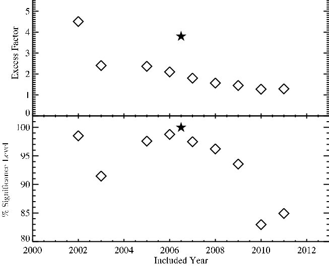
It is further illuminating to estimate the statistical significance of the Mg II enhancement along GRB sightlines as a function of historical time. Figure 8 shows the results of a Monte Carlo analysis for each year, where we include all GRBs from that year and any previous. Until the end of 2006 a significant () excess was present. Since that time, the statistical significance has steadily declined and the current full sample (which has several times the survey path of P06) has only a modest statistical significance. At present, we do not find a statistically significant difference in the incidence of strong Mg II absorbers between GRB and quasar sightlines.
V.3 Other Characteristics of the Mg II GRB Sample
In Fig. 9 we present the cumulative distributions of the equivalent widths and relative velocities for the strong Mg ii full sample. The latter is calculated assuming that these intervening systems are local to the GRB environments and are moving at such velocity towards the observer to mimic a lower redshift system [see also 20, for the intrinsic properties of a small sample of such systems]. As previously observed, more than of the intervening systems would require ejection velocities larger than km s-1, making very unlikely an intrinsic origin of these absorbers. Recently, [5], based on similar distribution of strong Mg ii absorbers along blazars, have suggested a possible theoretical model for producing such high relative velocities.
The red curves represent similar quantities from our Monte Carlo analysis of the QSO sightlines. A KS-test analysis shows for both metrics that the GRB and QSO absorbers are consistent with having been drawn from the same parent population ( and , for the and the projected velocity respectively).
VI Discussion and Conclusion
We have presented the largest compilation to date of GRB spectroscopic data, more than one hundred spectra including data from previous published works, proprietary datasets, and publicly available datasets not yet published. We have leveraged this dataset to investigate the puzzling excess of strong Mg ii absorbers along GRB sightlines as first noted by [63]. Most importantly, we have performed such analysis on a fully independent dataset to the original P06 study in order to test their findings.
This independent sample, our Sample I, comprises 83 GRB lines of sights, yielding a redshift path length over the interval . Along these spectra, we detect only 8 absorbers, for a total incidence of strong Mg II absorbers (Å) of . This incidence lies in good agreement with estimations along QSO lines of sight taken from the latest work by [83] (). No excess has been identified in the independent sample and, therefore, we do not confirm the original findings of P06 that an excess of Mg II absorbers lie along GRB sightlines.
It is likely that the earlier works on the incidence of Mg II absorption along GRB sightlines were biased by a remarkable, statistical fluke. In particular, the presence of a small set of lines of sight with multiple absorbers appears to have driven the results [39, as suggested by].
Even including the original P06 data (i.e. our full dataset, Sample F), which maximizes the redshift path coverage observed along GRBs sightlines (), we estimate , which corresponds to an excess of strong Mg ii absorbers by a factor over QSO sightlines (at c.l. for Poisson distribution). We tested the significance of this excess using a Monte Carlo analysis and find that of random QSO samples exhibit as many absorbers as the GRB survey. This suggests the null hypothesis is ruled out at confidence level. In conclusion, the data no longer demand a different incidence of strong Mg II absorption along GRB and QSO sightlines.
We wish to emphasize that the P06 analysis was not inherently flawed. Indeed, if we restrict our analysis to the set of high-resolution data, which has large overlap with the P06 sample, we find a significant excess ( times) at a high statistical significance (). At face value, this could suggest that we have underestimated for the low-resolution sample, e.g. because we mis-estimated our sensitivity to 1Å absorbers. Our sample of low-resolution data, however, includes a large diversity of S/N. In order to investigate the effect of these diversity on our detection rate, we degraded the spectra in Sample H to the lowest S/N and resolution for which we are able to estimate the redshift path length (e.g. the ALFOSC spectrum of GRB 050802, which has S/N=7 and ): all the strong Mg ii doublets could still be detected at level. Furthermore, we have identified many additional Mg II absorbers in these spectra (Table 5) where the selection criteria are not fully satisfied. We also established our completeness level and the reliability of our automatic searching algorithm creating a larger (5000) set of spectra, derived by the original full sample, where we randomly injected mocked doublet profiles with different equivalent widths. The automatic identification process recovered of the mocked features. At this stage, we suspect that the few lines of sight observed with high-resolution spectrographs were simply “peculiar” with respect the presence of strong Mg ii doublets. Surely a larger collection of such data (e.g. the sample building with X-Shooter) will allow for an independent test of the high-resolution results.
It is also worth noting, in this context, that other authors have explored whether the brightness of the GRB afterglow correlates with the presence of intervening Mg II absorption, i.e. to bias the observations towards such sightlines. [39] have investigated the optical properties of these GRBs in relation to the presence/absence of Mg ii absorbers and the possibility that GRB optical afterglows brightness may be boosted due to gravitational lensing [59, 48, see]. In particular they compared the absolute mean -band magnitude (estimated at one day post-burst and normalized at ) of GRB with strong absorbers and without (which usually present weak absorbers). For this purpose they used afterglow spectra obtained with echelle spectrographs which provide high-. No appreciable difference was noticed between the two samples. While we defer the reader to [47] for a quantitative estimate of possible gravitational lensing effects, we note that considering only the lines of sight with strong absorbers, our Sample H extends the original work of [39] by only one object, leading to inconclusive progress on this aspect due small size samples.
Moreover, we compared the equivalent width distribution of the detected absorbers in our Sample F and our Monte Carlo analysis: a Kolmogorov-Smirnov test shows that no significant difference is present between the two samples (). Similarly, if considering the relative velocity of the two populations of absorbers as they were, instead of intervening, moving at high velocity towards the observer so as to mimic a lower redshift we also do not find any particular difference (), further disfavouring an intrinsic nature for the absorbers.
Undoubtedly, the most robust results are obtained from high S/N, high resolution (Echelle or Echellette) data, of which we only have a limited sample for GRB afterglows to-date. For this reason new samples (such as that being gathered by X-shooter) obtained at high resolution will provide an important test of our conclusions.
References
- [1] Barth, A. J. et al. 2003, ApJ, 584, L47
- [2] Barthelmy, S. D., Butterworth, P., Cline, T. L., Gehrels, N., Fishman, G. J., Kouveliotou, C., & Meegan, C. A. 1995, Ap&SS, 231, 235
- [3] Barton, E. J. & Cooke, J. 2009, AJ, 138, 1817
- [4] Bergeron, J. 1986, A&A, 155, L8
- [5] Bergeron, J., Boissé, P., & Ménard, B. 2011, A&A, 525, A51
- [6] Bordoloi, R. et al. 2011, ApJ, 743, 10
- [7] Bowen, D. V., Blades, J. C., & Pettini, M. 1995, ApJ, 448, 634
- [8] Bowen, D. V. & Chelouche, D. 2011, ApJ, 727, 47
- [9] Budzynski, J. M. & Hewett, P. C. 2011, MNRAS, 416, 1871
- [10] Castro, S., Galama, T. J., Harrison, F. A., Holtzman, J. A., Bloom, J. S., Djorgovski, S. G., & Kulkarni, S. R. 2003, ApJ, 586, 128
- [11] Cenko, S. B. et al. 2008, ApJ, 677, 441
- [12] Chen, H.-W. 2012, MNRAS, 419, 3039
- [13] Chen, H.-W., Helsby, J. E., Gauthier, J.-R., Shectman, S. A., Thompson, I. B., & Tinker, J. L. 2010, ApJ, 714, 1521
- [14] Chen, H.-W. et al. 2009, ApJ, 691, 152
- [15] Chen, H.-W. & Tinker, J. L. 2008, ApJ, 687, 745
- [16] Christensen, L., Fynbo, J. P. U., Prochaska, J. X., Thöne, C. C., de Ugarte Postigo, A., & Jakobsson, P. 2011, ApJ, 727, 73
- [17] Cooksey, K. L., Thom, C., Prochaska, J. X., & Chen, H.-W. 2010, ApJ, 708, 868
- [18] Cucchiara, A. 2010, PhD thesis, The Pennsylvania State University
- [19] Cucchiara, A. et al. 2011a, ApJ, 743, 154
- [20] Cucchiara, A., Jones, T., Charlton, J. C., Fox, D. B., Einsig, D., & Narayanan, A. 2009, ApJ, 697, 345
- [21] Cucchiara, A. et al. 2011b, ApJ, 736, 7
- [22] de Ugarte Postigo, A. et al. 2012a, ArXiv e-prints
- [23] — 2012b, A&A, 538, A44
- [24] de Ugarte Postigo, A., Thöne, C. C., Goldoni, P., Fynbo, J. P. U., & X-shooter GRB Collaboration 2011, Astronomische Nachrichten, 332, 297
- [25] D’Elia, V., Campana, S., Covino, S., D’Avanzo, P., Piranomonte, S., & Tagliaferri, G. 2011, MNRAS, 418, 680
- [26] D’Elia, V. et al. 2010, A&A, 523, A36
- [27] Frank, S., Bentz, M. C., Stanek, K. Z., Mathur, S., Dietrich, M., Peterson, B. M., & Atlee, D. W. 2007, Ap&SS, 312, 325
- [28] Fynbo, J. P. U. et al. 2009, ApJS, 185, 526
- [29] Gehrels, N. et al. 2004, ApJ, 611, 1005
- [30] Gehrels, N., Ramirez-Ruiz, E., & Fox, D. B. 2009, ARA&A, 47, 567
- [31] Goldoni, P., Royer, F., François, P., Horrobin, M., Blanc, G., Vernet, J., Modigliani, A., & Larsen, J. 2006, in Society of Photo-Optical Instrumentation Engineers (SPIE) Conference Series, Vol. 6269, Society of Photo-Optical Instrumentation Engineers (SPIE) Conference Series
- [32] Greiner, J. et al. 2008, PASP, 120, 405
- [33] Hook, I. M., Jørgensen, I., Allington-Smith, J. R., Davies, R. L., Metcalfe, N., Murowinski, R. G., & Crampton, D. 2004, PASP, 116, 425
- [34] Horne, K. 1986, PASP, 98, 609
- [35] Jakobsson, P. et al. 2006, A&A, 460, L13
- [36] — 2004, A&A, 427, 785
- [37] Kacprzak, G. G., Churchill, C. W., & Nielsen, N. M. 2012, ApJ, 760, L7
- [38] Kacprzak, G. G., Churchill, C. W., Steidel, C. C., & Murphy, M. T. 2008, AJ, 135, 922
- [39] Kann, D. A. et al. 2010, ApJ, 720, 1513
- [40] Kawai, N. et al. 2006, Nature, 440, 184
- [41] Klose, S. et al. 2004a, AJ, 128, 1942
- [42] — 2004b, AJ, 128, 1942
- [43] Lanzetta, K. M., Turnshek, D. A., & Wolfe, A. M. 1987, ApJ, 322, 739
- [44] Lawther, D., Paarup, T., Schmidt, M., Vestergaard, M., Hjorth, J., & Malesani, D. 2012, A&A, 546, A67
- [45] López, G. & Chen, H.-W. 2012, MNRAS, 419, 3553
- [46] Matejek, M. S. & Simcoe, R. A. 2012, ArXiv e-prints
- [47] Ménard, B. 2005, ApJ, 630, 28
- [48] Ménard, B., Nestor, D., Turnshek, D., Quider, A., Richards, G., Chelouche, D., & Rao, S. 2008, MNRAS, 385, 1053
- [49] Ménard, B., Wild, V., Nestor, D., Quider, A., Zibetti, S., Rao, S., & Turnshek, D. 2011, MNRAS, 417, 801
- [50] Metzger, M. R., Djorgovski, S. G., Kulkarni, S. R., Steidel, C. C., Adelberger, K. L., Frail, D. A., Costa, E., & Frontera, F. 1997, Nature, 387, 878
- [51] Milvang-Jensen, B., Fynbo, J. P. U., Malesani, D., Hjorth, J., Jakobsson, P., & Møller, P. 2012, ApJ, 756, 25
- [52] Mirabal, N. et al. 2002, ApJ, 578, 818
- [53] Nestor, D. B., Johnson, B. D., Wild, V., Ménard, B., Turnshek, D. A., Rao, S., & Pettini, M. 2011, MNRAS, 412, 1559
- [54] Nestor, D. B., Turnshek, D. A., & Rao, S. M. 2005, ApJ, 628, 637
- [55] Perley, D. A. et al. 2008, ApJ, 688, 470
- [56] Pollack, L. K., Chen, H.-W., Prochaska, J. X., & Bloom, J. S. 2009, ApJ, 701, 1605
- [57] Porciani, C. & Madau, P. 2001, ApJ, 548, 522
- [58] Porciani, C., Viel, M., & Lilly, S. J. 2007a, ApJ, 659, 218
- [59] — 2007b, ApJ, 659, 218
- [60] Prochaska, J. X., Chen, H.-W., & Bloom, J. S. 2006, ApJ, 648, 95
- [61] Prochaska, J. X. et al. 2007, ApJS, 168, 231
- [62] Prochter, G. E., Prochaska, J. X., & Burles, S. M. 2006a, ApJ, 639, 766
- [63] Prochter, G. E. et al. 2006b, ApJ, 648, L93
- [64] Quider, A. M., Nestor, D. B., Turnshek, D. A., Rao, S. M., Monier, E. M., Weyant, A. N., & Busche, J. R. 2011, AJ, 141, 137
- [65] Rapoport, S., Onken, C. A., Schmidt, B. P., Wyithe, J. S. B., Tucker, B. E., & Levan, A. J. 2011, ArXiv e-prints
- [66] Rodríguez Hidalgo, P., Wessels, K., Charlton, J., Narayanan, A., Mshar, A., Cucchiara, A., & Jones, T. 2012, ArXiv e-prints
- [67] Rubin, K. H. R., Prochaska, J. X., Ménard, B., Murray, N., Kasen, D., Koo, D. C., & Phillips, A. C. 2011, ApJ, 728, 55
- [68] Salvaterra, R. et al. 2009, Nature, 461, 1258
- [69] Schulze, S. et al. 2012, ArXiv e-prints
- [70] Simcoe, R. A. et al. 2011, ApJ, 743, 21
- [71] Steidel, C. C. 1993, in Astronomical Society of the Pacific Conference Series, Vol. 49, Galaxy Evolution. The Milky Way Perspective, ed. S. R. Majewski, 227
- [72] Steidel, C. C. & Sargent, W. L. W. 1992, ApJS, 80, 1
- [73] Tanvir, N. R. et al. 2009, Nature, 461, 1254
- [74] Thoene, C. C., de Ugarte Postigo, A., Vreeswijk, P. M., Malesani, D., & Jakobsson, P. 2008, GRB Coordinates Network, 8058, 1
- [75] van Dokkum, P. G. 2001, PASP, 113, 1420
- [76] Vergani, S. D., Petitjean, P., Ledoux, C., Vreeswijk, P., Smette, A., & Meurs, E. J. A. 2009, A&A, 503, 771
- [77] Vestrand, W. T. et al. 2002, in Society of Photo-Optical Instrumentation Engineers (SPIE) Conference Series, Vol. 4845, Society of Photo-Optical Instrumentation Engineers (SPIE) Conference Series, ed. R. I. Kibrick, 126–136
- [78] Vreeswijk, P. M. et al. 2004, A&A, 419, 927
- [79] — 2007, A&A, 468, 83
- [80] Vreeswijk, P. M., Møller, P., & Fynbo, J. P. U. 2003, A&A, 409, L5
- [81] Werk, J. K., Prochaska, J. X., Thom, C., Tumlinson, J., Tripp, T. M., O’Meara, J. M., & Meiring, J. D. 2012, ApJS, 198, 3
- [82] York, D. G. et al. 2000, AJ, 120, 1579
- [83] Zhu, G. B. & Menard, B. 2012, arXiv:1211.6215
- [84] Zibetti, S., Ménard, B., Nestor, D. B., Quider, A. M., Rao, S. M., & Turnshek, D. A. 2007, ApJ, 658, 161
| GRB | Telescope | Instrument | Resolution | Reference | ||
|---|---|---|---|---|---|---|
| (Å) | ||||||
| 111229A | 1.380 | Gemini | GMOS | this work | ||
| 111107A | 2.893 | Gemini | GMOS | this work | ||
| 111008A | 4.989 | Gemini | GMOS | this work | ||
| 110918A | 0.982 | Gemini | GMOS | this work | ||
| 110731A | 2.830 | Gemini | GMOS | this work | ||
| 110726A | 1.036 | Gemini | GMOS | this work | ||
| 110213B | 1.083 | Gemini | GMOS | this work | ||
| 110213A | 1.460 | Bok | FAST | (4) | ||
| 110205A | 2.214 | Lick | KAST | 14 | (4) | |
| 100906A | 1.727 | Gemini | GMOS | this work | ||
| 100901A | 1.408 | Gemini | GMOS | this work | ||
| 100814A | 1.438 | MAGELLAN | MagE | 10 | this work | |
| 100513A | 4.798 | Gemini | GMOS | this work | ||
| 100418A | 0.624 | VLT | X-Shooter | 0.86/0.72/2∗ | (19) | |
| 100414A | 1.368 | Gemini | GMOS | this work | ||
| 100302A | 4.813 | Gemini | GMOS | this work | ||
| 100219A | 4.667 | Gemini | GMOS | this work | ||
| 091208B | 1.063 | Gemini | GMOS | (2) | ||
| 091109A | 3.076 | VLT | FORS2 | this work | ||
| 091029 | 2.752 | Gemini | GMOS | this work | ||
| 091024 | 1.092 | Gemini | GMOS | (2) | ||
| 091020A | 1.713 | NOT | ALFOSC | this work | ||
| 090926A | 2.106 | VLT | X-Shooter | (6) | ||
| 090902B | 1.822 | Gemini | GMOS | this work | ||
| 090812A | 2.454 | VLT | FORS2 | (18) | ||
| 090529A | 2.625 | VLT | FORS2 | (18) | ||
| 090519A | 3.851 | VLT | FORS2 | (18) | ||
| 090516A | 4.109 | VLT | FORS2 | (18) | ||
| 090426 | 2.609 | Keck | LRIS | 8 | this work | |
| 090424 | 0.544 | Gemini | GMOS | this work | ||
| 090323 | 3.567 | Gemini | GMOS | this work | ||
| 090313 | 3.375 | Gemini | GMOS | this work | ||
| 081222 | 2.771 | Gemini | GMOS | this work | ||
| 081029 | 3.847 | Gemini | GMOS | (2) | ||
| 081008 | 1.967 | Gemini | GMOS | (2) | ||
| 081007 | 0.529 | Gemini | GMOS | (2) | ||
| 080928 | 1.690 | Gemini/VLT | GMOS/FORS2 | (2)/(3) | ||
| 080916A | 0.689 | VLT | FORS1 | (18) | ||
| 080913A | 6.700 | VLT | FORS2 | (13) | ||
| 080905B | 2.374 | VLT | FORS1 | 13 | (18) | |
| 080810 | 3.350 | Keck | HIRES | 16 | (18) | |
| 080805 | 1.505 | VLT | FORS2 | (3) | ||
| 080804 | 2.205 | Gemini | GMOS | (2) | ||
| 080721 | 2.608 | TNG | Dolores | (18) | ||
| 080710 | 0.845 | Gemini | GMOS | (2) | ||
| 080707 | 1.234 | VLT | FORS1 | (3) | ||
| 080607 | 3.036 | Keck | LRIS | 11 | (3) | |
| 080605A | 1.639 | VLT | FORS2 | (3) | ||
| 080604 | 1.416 | Gemini | GMOS | (2) | ||
| 080603B | 2.686 | NOT | ALFOSC | (3) | ||
| 080603A | 1.688 | Gemini | GMOS | (2) | ||
| 080520 | 1.545 | VLT | FORS2 | (3) | ||
| 080413B | 1.100 | Gemini | GMOS | (2) | ||
| 080413A | 2.433 | Gemini | GMOS | (2)/(9) | ||
| 080411 | 1.030 | VLT | FORS1 | (18) | ||
| 080330 | 1.513 | NOT | ALFOSC | (3) | ||
| 080319C | 1.949 | Gemini | GMOS | (2) | ||
| 080319B | 0.937 | Gemini/VLT | GMOS/UVES | (2)/(9) | ||
| 080310A | 2.4272 | VLT | UVES | 15 | (9) | |
| 080210 | 2.6419 | VLT | FORS2 | (3) | ||
| 071122 | 1.141 | Gemini | GMOS | (2) | ||
| 071117 | 1.334 | VLT | FORS1 | (3) | ||
| 071112C | 0.823 | Gemini | GMOS | (2) | ||
| 071031 | 2.692 | VLT | UVES/FORS2 | (3) | ||
| 071020 | 2.145 | VLT | FORS2 | (3) | ||
| 071010B | 0.947 | Gemini | GMOS | (2) | ||
| 071003 | 1.6044 | Keck | LRIS | 34 | (20) | |
| 070810A | 2.170 | Keck | LRIS | 6 | (21) | |
| 070802 | 2.453 | VLT | FORS2 | (3) | ||
| 070721B | 3.626 | VLT | FORS2 | (18) | ||
| 070611 | 2.039 | VLT | FORS2 | (3) | ||
| 070529 | 2.498 | Gemini | GMOS | (2) | ||
| 070506 | 2.306 | VLT | FORS1 | (3) | ||
| 070411 | 2.954 | VLT | FORS1 | (3) | ||
| 070318 | 0.836 | Gemini | GMOS | (2) | ||
| 070306 | 1.496 | VLT | FORS2 | (3) | ||
| 070125 | 1.547 | Gemini/VLT | GMOS/FORS1 | (10)/(3) | ||
| 070110 | 2.352 | VLT | FORS2 | (3) | ||
| 061121 | 1.314 | Keck | LRIS | 28 | (3) | |
| 061110B | 3.434 | VLT | FORS1 | (3) | ||
| 061110A | 0.758 | VLT | FORS1 | (3) | ||
| 061007 | 1.261 | VLT | FORS1 | (3) | ||
| 060927 | 5.468 | VLT | FORS1 | (1) | ||
| 060926 | 3.205 | VLT | FORS1 | (1) | ||
| 060908 | 1.884 | Gemini | GMOS | this work | ||
| 060906 | 3.686 | VLT | FORS1 | 13 | (1) | |
| 060904B | 0.703 | VLT | FORS1 | (18) | ||
| 060729 | 0.543 | Gemini | GMOS | (2) | ||
| 060714 | 2.711 | VLT | FORS1 | (3) | ||
| 060708 | 1.923 | VLT | FORS2 | (3) | ||
| 060707 | 3.425 | VLT | FORS2 | (3) | ||
| 060607A | 3.047 | VLT | UVES | 43 | (9) | |
| 060526 | 3.221 | VLT | FORS1 | (1) | ||
| 060522 | 5.111 | Keck | LRIS | 2.3 | (1) | |
| 060512 | 2.092 | VLT | FORS1 | 3 | (3) | |
| 060510B | 4.922 | Gemini | GMOS | (2) | ||
| 060502A | 1.515 | Gemini | GMOS | (2) | ||
| 060418 | 1.489 | Gemini/VLT | GMOS/UVES | (2)/(11) | ||
| 060210 | 3.912 | Gemini | GMOS | (2) | ||
| 060206 | 4.046 | NOT | ALFOSC | (3) | ||
| 060124 | 2.296 | Keck | ESI | 8 | (3) | |
| 060115 | 3.5328 | VLT | FORS1 | (3) | ||
| 051111 | 1.5489 | Keck | HIRES | 20 | (12) | |
| 050922C | 2.1996 | VLT | UVES | 12 | (9) | |
| 050908 | 3.339 | Gemini/Keck | GMOS/Deimos | (2)/this work | ||
| 050820 | 2.614 | VLT | UVES | 23 | (9) | |
| 050802 | 1.711 | NOT | ALFOSC | (3) | ||
| 050801 | 1.559 | Keck | LRIS | 5 | (3) | |
| 050730 | 3.9687 | VLT | UVES | 40 | (9) | |
| 050401 | 2.896 | VLT | FORS2 | (3) | ||
| 050319 | 3.240 | NOT | ALFOSC | (3) | ||
| 030429 | 2.655 | VLT | FORS1 | (1) | ||
| 030323 | 3.372 | VLT | FORS1 | (13) | ||
| 030226 | 1.986 | VLT | FORS1 | (14) | ||
| 021004 | 2.323 | VLT | UVES | 40 | (9) | |
| 020813 | 1.255 | VLT | UVES | (15) | ||
| 010222 | 1.477 | Keck | ESI | 4 | (16) | |
| 000926 | 2.038 | Keck | ESI | 12 | (17) |
| Number a | |||||
|---|---|---|---|---|---|
| of GRBs | |||||
| Sample I | 83 | 44.9 | 8 | 0.26 | |
| Sample F | 95 | 55.5 | 20 | 0.24 | |
| Sample H | 18 | 20.3 | 13 | 0.25 | |
| Sample L | 79 | 35.3 | 7 | 0.12 |
Note. — Summary of our Mg ii search: the sample name and the number of lines of sight included are listed in the first two columns; the total redshift path density explored and the number of absorbers identified are listed in the third and forth column. Based on these we could determine the incidence of the absorbers in each sample and compare it with the expected incidence along our QSOs sample (last two columns).
| Description | (Å) | Description | (Å) |
|---|---|---|---|
| N v | 1238,1242 | C i | 1560, |
| S ii | 1250,1253,1259 | Fe ii | 1608,1611,2249,2260,2344,2374,2382,2586,2600 |
| Si ii | 1260,1304,1526,1808 | Al ii | 1670 |
| Si ii* | 1264,1309,1533,1816 | Al iii | 1854,862 |
| O i | 1302 | Cr ii | 2017,2026,2056,2066 |
| Ni ii | 1317,1370,1454,1703,1709,1741,1751 | Zn ii | 2026,2062 |
| C ii | 1334 | Ni ii* | 2217 |
| C ii* | 1335 | Mn ii | 2576,2594,2606 |
| Si iv | 1393,1402 | Band Ba | |
| C iv | 1548,1550 | Band Aa | |
| Atm. Banda | Atm. Banda |
| GRB | |||
|---|---|---|---|
| 030226 | 1.986 | 1.30132 | 1.31706 |
| 1.32636 | 1.32922 | ||
| 1.35426 | 1.38430 | ||
| 1.41005 | 1.41935 | ||
| 1.42936 | 1.45655 | ||
| 1.46656 | 1.48158 | ||
| 1.50161 | 1.54667 | ||
| 1.55669 | 1.62393 | ||
| 1.64038 | 1.64682 | ||
| 1.66971 | 1.71119 | ||
| 1.72407 | 1.76127 | ||
| 1.77200 | 1.77700 | ||
| 1.78773 | 1.81134 | ||
| 1.82922 | 1.85211 | ||
| 1.86284 | 1.86356 | ||
| 1.87428 | 1.92364 | ||
| 1.94367 | 1.97300 | ||
| 1.99231 | 2.14664 | ||
| 2.16738 | 2.18741 | ||
| 2.20959 | 2.35908 | ||
| 2.37124 | 2.39413 | ||
| 2.41774 | 2.44850 | ||
| 2.48927 | 2.48999 | ||
| 2.50644 | 2.52718 | ||
| 2.54793 | 2.70959 | ||
| 2.75894 | 2.75966 | ||
| 2.78040 | 2.78112 | ||
| 2.78684 | 2.90057 |
| GRB | Statistical | Other | ||||
|---|---|---|---|---|---|---|
| (Å) | (Å) | sample | transition | |||
| 010222 | F,H | Fe ii | ||||
| 020813 | F,H | Mg i,Fe ii | ||||
| 021004c | N | Mg i,Fe ii | ||||
| F,H | Mg i,Mn ii,Fe ii | |||||
| F,H | Mg i, Fe ii,Mn ii | |||||
| 030226d | N | Al ii | ||||
| N | Mg i, C iv,Si ii | |||||
| 050730c | N | Mg i,Fe ii | ||||
| N | Si ii,Al ii,Fe ii,Mg i | |||||
| 050820c | F,H | Mg i | ||||
| F,H | Mg i,Fe ii,Al iii | |||||
| N | Mg i,Fe ii,Zn ii,Si ii | |||||
| N | Fe ii,Si ii,Zn ii,C iv | |||||
| 050908 | F,H | Fe ii | ||||
| 050922Cc | N | Mg i,Fe ii | ||||
| N | Mg i,Fe ii | |||||
| N | C iv,Fe ii | |||||
| 051111 | F,H | Mg i,Fe ii | ||||
| N | Mg i | |||||
| 060418b | F,H | Mg i,Fe ii,Zn ii,Al iii,Al ii | ||||
| F,H | Fe ii | |||||
| F,H | Fe ii | |||||
| 060502A | F,L,I | Mg i | ||||
| N | ||||||
| F,L,I | Fe i,Mn ii,Mg i | |||||
| 060607Ac | N | Fe ii | ||||
| F,H,I | Mg i,Fe ii,Al iii | |||||
| N | Fe ii,Al iii,Al ii,C iv,Si ii,Si iv | |||||
| 060906 | N | Mg i | ||||
| 060926 | N | Mg i,Fe i | ||||
| N | Mg i,Fe ii,Mn ii | |||||
| N | Mg i | |||||
| 061007 | N | Mg i,Fe ii,Mn ii | ||||
| 070529 | N | |||||
| 070506 | N | Al iii | ||||
| 070611 | N | Mg i,Fe ii | ||||
| 070802 | N | Al ii,Ni ii,Mg i,Fe ii | ||||
| N | Ni ii,Al iii,Cr ii,Fe ii | |||||
| 071003 | F,L,I | Mg i | ||||
| N | Mg i | |||||
| N | Mg i | |||||
| 071031c | 0.206 (0.008) | N | Fe ii | |||
| 0.586 (0.052) | N | Fe ii,Al iii,C iv | ||||
| 0.612 (0.016) | N | Mg i,Fe ii | ||||
| 080310c | 0.366 (0.016) | N | Mg i,Fe ii,Al ii,Si ii,C iv | |||
| 080319Bc | 0.350 (0.002) | N | Mg i,Fe ii | |||
| 0.029 (0.001) | N | Mg i,Fe ii | ||||
| 0.736 (0.003) | F,H,I | Mg i,Fe ii | ||||
| 0.039 (0.002) | N | Fe ii | ||||
| 080319C | N | Fe ii,Mn ii | ||||
| 080603A | F,L,I | Mg i,Fe ii | ||||
| N | Fe i | |||||
| 080605 | F,L,I | Fe ii | ||||
| 080607A | F,L,I | Mg i | ||||
| 080805A | N | Mn ii,Fe ii | ||||
| 080905B | N | Mg i | ||||
| 080928 | N | Mg i,Fe ii | ||||
| 081222 | N | Mg i,Fe ii | ||||
| F,L,I | Fe ii | |||||
| 091208B | N | Mg i | ||||
| 100814A | N | Mg i | ||||
| 100901A | N | Fe ii,Mg i | ||||
| 100906A | N | |||||
| 110918A | N | Mg i,Fe ii |