跳到论文正文
W Papers独立论文阅读器 arXiv:1211.6162 论文正文 计算阅读时间 · 0%
引用这篇论文根据当前论文元数据生成,正式投稿前建议核对。


License: arXiv.org perpetual non-exclusive license
arXiv:1211.6162v2 [math.OC] 28 Nov 2012

Quality of Information Maximization for Wireless Networks via a Fully Separable Quadratic PolicyThanks: This material was presented in part at the IEEE International Conference on Communications, Ottawa, Canada, June 2012 [1]. This material is supported in part by one or more of the following: the NSF Career grant CCF-0747525, the Network Science Collaborative Technology Alliance sponsored by the U.S. Army Research Laboratory W911NF-09-2-0053.

Sucha Supittayapornpong,  Michael J. Neely Affiliation:  Affiliation: Department of Electrical Engineering
University of Southern California
Los Angeles, California
Email: supittay@usc.edu,  mjneely@usc.edu
Affiliation: 
Abstract

An information collection problem in a wireless network with random events is considered. Wireless devices report on each event using one of multiple reporting formats. Each format has a different quality and uses different data lengths. Delivering all data in the highest quality format can overload system resources. The goal is to make intelligent format selection and routing decisions to maximize time-averaged information quality subject to network stability. Lyapunov optimization theory can be used to solve such a problem by repeatedly minimizing the linear terms of a quadratic drift-plus-penalty expression. To reduce delays, this paper proposes a novel extension of this technique that preserves the quadratic nature of the drift minimization while maintaining a fully separable structure. In addition, to avoid high queuing delay, paths are restricted to at most two hops. The resulting algorithm can push average information quality arbitrarily close to optimum, with a trade-off in queue backlog. The algorithm compares favorably to the basic drift-plus-penalty scheme in terms of backlog and delay. Furthermore, the technique is generalized to solve linear programs and yields smoother results than the standard drift-plus-penalty scheme.

I Introduction

This paper investigates dynamic scheduling and data format selection in a network where multiple wireless devices, such as smart phones, report information to a receiver station. The devices together act as a pervasive pool of information about the network environment. Such scenarios have been recently considered, for example, in applications of social sensing [2] and personal environment monitoring [3, 4]. Sending all information in the highest quality format can quickly overload network resources. Thus, it is often more important to optimize the quality of information, as defined by an end-user, rather than the raw number of bits that are sent. The case for quality-aware networking is made in [5, 6, 7]. Network management with quality of information awareness for wireless sensor networks is considered in [8]. More recently, quality metrics of accuracy and credibility are considered in [9, 10] using simplified models that do not consider the actual dynamics of a wireless network.

In this paper, we extend the quality-aware format selection problem in [10] to a dynamic network setting. We particularly focus on distributed algorithms for routing, scheduling, and format selection that jointly optimize quality of information. Specifically, we assume that random events occur over time in the network environment, and these can be sensed by one or more of the wireless devices, perhaps at different sensing qualities. At the transport layer, each device selects one of multiple reporting formats, such as a video clip at one of several resolution options, an audio clip, or a text message. Information quality depends on the selected format. For example, higher quality formats use messages with larger bit lengths. The resulting bits are handed to the network layer at each device and must be delivered to the receiver station over possibly time-varying channels. This delivery can be a direct transmission from a device to the receiver station via an uplink channel, or can take a two-hop path that utilizes another device as relay (we restrict paths to at most two-hops for tight control over network delays). An example is a single-cell wireless network with multiple smart phones and one base station, where each smart phone has 3G capability for uplink transmission and Wi-Fi capability for device-to-device relay transmission.

Such a problem can be cast as a stochastic network optimization and solved using Lyapunov optimization theory. A “standard” method is to minimize a linear term in a quadratic drift-plus-penalty expression [11, 12]. This can be shown to yield algorithms that converge to optimal average utility with a trade-off in average queue size. The linearization is useful for enabling decisions to be separated at each device. However, it can lead to larger queue sizes and delays. In this work, we propose a novel method that uses a quadratic minimization for the drift-plus-penalty expression, yet still allows separability of the decisions. This results in an algorithm that maintains distributed decisions across all devices for format selection and routing, similar to the standard (linearized) drift-plus-penalty approach, but reduces overall queue size.

For the derived algorithm, each device observes its input queue length and then selects a format to report an event according to a simple rule. The routing decision for each group of bits is determined at each device by considering its input, uplink, and relay queues. Then, allocation of channel resources for direct transmission is determined from a receiver station after observing current uplink queues and channel conditions. For the relay transmission, an optimization problem involving relay queues, uplink queues and channel conditions is solved at the receiver station to determine an optimal transmission decision. This process can be decentralized if all channels are orthogonal.

Our analysis shows that the standard drift-plus-penalty algorithm and our new algorithm both converge to the optimal quality of information. The analysis also shows a deterministic maximum size of each queue. Simulations show that the new algorithm has a significant savings in queue length which implies reduction of average delay.

Because of the generality of the novel method, it is applied to solve linear programs in the last section. Linear programs are a special case of the stochastic problems treated in [12], and hence can be solved by the (linearized) drift plus penalty method of Lyapunov optimization theory. This is done in [13] to distributively solve linear programs over graphs. The current paper applies our novel quadratic drift-plus-penalty algorithm to linear programs to produce smoother results and faster convergence. Although a solution of this new technique is the time-average of results from multiple iterations, it is different from the “dual averaging” method of [14] which has a different problem construction, and from the “alternating direction method of multipliers” in [15] which arises from gradient descent methods rather than from Lyapunov optimization.

Thus, our contributions are threefold: (i) We formulate an important quality-of-information problem for reporting information in wireless systems. This problem is of recent interest and can be used in other contexts where “data deluge” issues require selectivity in reporting of information. (ii) We extend Lyapunov optimization theory by presenting a new algorithm that uses a quadratic minimization to reduce queue sizes while maintaining separability across decisions. This new technique is general and can be used to reduce queue sizes in other Lyapunov optimization problems. (iii) We illustrate the potential of the quadratic minimization for solving linear programs.

In the next section we formulate the problem. Sec. III derives the novel quadratic algorithm. Sec. IV analyzes its performance. Sec. V presents simulation results. Sec. VI illustrates how to solve linear programs. The conclusion is in Sec. VII.

II System Model

Consider a network with NN wireless devices that report information to a single receiver station. Let 𝒩={1,…,N}{\mathcal{N}}=\{1,\ldots,N\} be the set of devices. The receiver station is not part of the set 𝒩{\mathcal{N}} and can be viewed as “device 0.” A network with N=3N=3 devices is shown in Fig. 1. The system is slotted with fixed size slots t∈{0,1,2,…}t\in\{0,1,2,\ldots\}. Every slot, format selection decisions are made at the transport layer of each device, and routing and scheduling decisions are made at the network layer.

Refer to caption
Fig. 1: An example network with illustration of the internal queues Kn​(t)K_{n}(t), Qn​(t)Q_{n}(t), Jn​(t)J_{n}(t) for each device nn.

II-A Format Selection

A new event can occur on each slot. Events are observed with different levels of quality at each device. For example, some devices may be physically closer to the event and hence can deliver higher quality. On slot tt, each device n∈𝒩n\in{\mathcal{N}} selects a format fn​(t)f_{n}(t) from a set of available formats ℱ={0,1,…,F}{\mathcal{F}}=\{0,1,\ldots,F\}. Format selection affects quality and data lengths of the reported information. To model this, the event on slot tt is described by a vector of event characteristics (rn(f)​(t),dn(f)​(t))|n∈𝒩,f∈ℱ(r_{n}^{(f)}(t),d_{n}^{(f)}(t))|_{n\in{\mathcal{N}},f\in{\mathcal{F}}}. The value rn(f)​(t)r_{n}^{(f)}(t) is a numeric reward that is earned if device nn uses format ff to report on the event that occurs on slot tt. The value dn(f)​(t)d_{n}^{(f)}(t) is the amount of data units required for this choice. This data is injected into the network layer and must eventually be delivered to the receiver station. To allow a device nn not to report on an event, there is a “blank format” 0∈ℱ0\in{\mathcal{F}} such that (rn(0)​(t),dn(0)​(t))=(0,0)(r_{n}^{(0)}(t),d_{n}^{(0)}(t))=(0,0) for all slots tt and all devices n∈𝒩n\in{\mathcal{N}}. If a device nn does not observe the event on slot tt (which might occur if it is physically too far from the event), then (rn(f)​(t),dn(f)​(t))=(0,0)(r_{n}^{(f)}(t),d_{n}^{(f)}(t))=(0,0) for all formats f∈ℱf\in{\mathcal{F}}. If no event occurs on slot tt, then (rn(f)​(t),dn(f)​(t))=(0,0)(r_{n}^{(f)}(t),d_{n}^{(f)}(t))=(0,0) for all n∈𝒩n\in{\mathcal{N}} and f∈ℱf\in{\mathcal{F}}.

Rewards rn​(t)r_{n}(t) are assumed to be real numbers that satisfy 0≤rn​(t)≤rn(max)0\leq r_{n}(t)\leq r_{n}^{(\text{max})} for all tt, where rn(max)r_{n}^{(\text{max})} is a finite maximum. Data sizes dn​(t)d_{n}(t) are non-negative integers that satisfy 0≤dn​(t)≤dn(max)0\leq d_{n}(t)\leq d_{n}^{(\text{max})} for all tt, where dn(max)d_{n}^{(\text{max})} is a finite maximum. The vectors (rn(f)​(t),dn(f)​(t))|n∈𝒩,f∈ℱ(r_{n}^{(f)}(t),d_{n}^{(f)}(t))|_{n\in{\mathcal{N}},f\in{\mathcal{F}}} are independent and identically distributed (i.i.d.) over slots tt, and have a joint probability distribution over devices nn and formats ff that is arbitrary (subject to the above properties). This distribution is not necessarily known.

II-B Routing and Scheduling

At each device n∈𝒩n\in{\mathcal{N}}, the dn​(t)d_{n}(t) units of data generated by format selection are put into input queue Kn​(t)K_{n}(t). Each device has two orthogonal communication capabilities, called (direct) uplink transmission and (ad-hoc) relay transmission. The uplink transmission capability allows each device to communicate to the receiver station directly via an uplink channel. The relay capability allows communication between a device and its neighboring devices. To ensure all data takes at most two hops to the destination, the data in each queue Kn​(t)K_{n}(t) is internally routed to one of two queues Qn​(t)Q_{n}(t) and Jn​(t)J_{n}(t), respectively holding data for uplink and relay transmission (see Fig. 1). Data in queue Qn​(t)Q_{n}(t) must be transmitted directly to the receiver station, while data in queue Jn​(t)J_{n}(t) can be transmitted to another device kk, but is then placed in queue Qk​(t)Q_{k}(t) for that device. This is conceptually similar to the hop-count based queue architecture in [16].

In each slot tt, let sn(q)​(t)s_{n}^{(q)}(t) and sn(j)​(t)s_{n}^{(j)}(t) represent the amount of data in Kn​(t)K_{n}(t) that can be internally moved to Qn​(t)Q_{n}(t) and Jn​(t)J_{n}(t), respectively, as illustrated in Fig. 1. These decision variables are chosen within sets 𝒮n(q){\mathcal{S}}_{n}^{(q)} and 𝒮n(j){\mathcal{S}}_{n}^{(j)}, respectively, where:

𝒮n(q)\displaystyle{\mathcal{S}}_{n}^{(q)} ≜\displaystyle\triangleq {0,1,…,sn(q)​(max)}\displaystyle\{0,1,\dotsc,s_{n}^{(q){(\text{max})}}\}
𝒮n(j)\displaystyle{\mathcal{S}}_{n}^{(j)} ≜\displaystyle\triangleq {0,1,…,sn(j)​(max)}\displaystyle\{0,1,\dotsc,s_{n}^{(j){(\text{max})}}\}

where sn(q)​(max)s_{n}^{(q){(\text{max})}}, sn(j)​(max)s_{n}^{(j){(\text{max})}} are finite maximum values. Then the dynamics of Kn​(t)K_{n}(t) are:

Kn​(t+1)=max⁡[Kn​(t)−sn(q)​(t)−sn(j)​(t),0]+dn​(t)K_{n}(t+1)=\max[K_{n}(t)-s_{n}^{(q)}(t)-s_{n}^{(j)}(t),0]+d_{n}(t) (1)

As a minor technical detail that is useful later, the max⁡[⋯,0]\max[\dotsb,0] operation above allows the sn(q)​(t)s_{n}^{(q)}(t) and sn(j)​(t)s_{n}^{(j)}(t) decisions to sum to more than Kn​(t)K_{n}(t). The actual sn(q)​(act)​(t)s_{n}^{(q){(\text{act})}}(t) and sn(j)​(act)​(t)s_{n}^{(j){(\text{act})}}(t) data units moved from Kn​(t)K_{n}(t) can be any values that satisfy:

sn(q)​(act)​(t)+sn(j)​(act)​(t)=min⁡[Kn​(t),sn(q)​(t)+sn(j)​(t)]\displaystyle s_{n}^{(q){(\text{act})}}(t)+s_{n}^{(j){(\text{act})}}(t)=\min[K_{n}(t),s_{n}^{(q)}(t)+s_{n}^{(j)}(t)] (2)
0≤sn(q)​(act)​(t)≤sn(q)​(t)\displaystyle 0\leq s_{n}^{(q){(\text{act})}}(t)\leq s_{n}^{(q)}(t) (3)
0≤sn(j)​(act)​(t)≤sn(j)​(t)\displaystyle 0\leq s_{n}^{(j){(\text{act})}}(t)\leq s_{n}^{(j)}(t) (4)

Wireless transmission is assumed to be channel-aware, and decision options are determined by a vector 𝜼⁡(t){\boldsymbol{\eta}}(t) of current channel states in the network. Specifically, let un​(t)u_{n}(t) be the amount of uplink data that can be transmitted from device nn to the receiver station, and let 𝒖⁡(t)=(un​(t))|n∈𝒩{\boldsymbol{u}}(t)=(u_{n}(t))|_{n\in{\mathcal{N}}} be the vector of these transmission decisions. It is assumed that 𝒖⁡(t){\boldsymbol{u}}(t) is chosen every slot tt within a set 𝒰𝜼⁡(t){\mathcal{U}}_{{\boldsymbol{\eta}}(t)} that depends on the observed 𝜼⁡(t){\boldsymbol{\eta}}(t). Similarly, let an​m​(t)a_{nm}(t) be the amount of data selected for ad-hoc transmission between devices nn and mm, and let 𝒂⁡(t)=(an​m​(t))|n,m∈𝒩{\boldsymbol{a}}(t)=(a_{nm}(t))|_{n,m\in{\mathcal{N}}} and an​n​(t)=0a_{nn}(t)=0 for every tt and nn. These transmissions are assumed to be orthogonal to the uplink transmissions. Every slot tt, the 𝒂⁡(t){\boldsymbol{a}}(t) vector is chosen within a set 𝒜𝜼⁡(t){\mathcal{A}}_{{\boldsymbol{\eta}}(t)} that depends on the observed 𝜼⁡(t){\boldsymbol{\eta}}(t). The sets 𝒰𝜼⁡(t){\mathcal{U}}_{{\boldsymbol{\eta}}(t)} and 𝒜𝜼⁡(t){\mathcal{A}}_{{\boldsymbol{\eta}}(t)} depend on the resource allocation, modulation, and coding options for transmission. If each uplink channel is orthogonal then set 𝒰𝜼⁡(t){\mathcal{U}}_{{\boldsymbol{\eta}}(t)} can be decomposed into a set product of individual options for each uplink, where each option depends on the component of 𝜼⁡(t){\boldsymbol{\eta}}(t) that represents its own uplink channel. Orthogonal relay links can be treated similarly.

The dynamics of relay queue Jn​(t)J_{n}(t) are:

Jn​(t+1)=max⁡[Jn​(t)−∑m∈𝒩​an​m​(t)+sn(j)​(act)​(t),0].J_{n}(t+1)=\max{\left[{J_{n}(t)-\mbox{$\sum_{m\in{\mathcal{N}}}$}a_{nm}(t)+s_{n}^{(j){(\text{act})}}(t),0}\right]}. (5)

As before, the actual amount of data an​m(act)​(t)a_{nm}^{(\text{act})}(t) satisfies:

∑m∈𝒩​an​m(act)​(t)=min⁡(Jn​(t)+sn(j)​(act)​(t),∑m∈𝒩​an​m​(t))\displaystyle\mbox{$\sum_{m\in{\mathcal{N}}}$}a_{nm}^{(\text{act})}(t)=\min\Bigl(J_{n}(t)+s_{n}^{(j){(\text{act})}}(t),\mbox{$\sum_{m\in{\mathcal{N}}}$}a_{nm}(t)\Bigr) (6)
0≤an​m(act)​(t)≤an​m​(t)for​m∈𝒩.\displaystyle 0\leq a_{nm}^{(\text{act})}(t)\leq a_{nm}(t)\quad\quad\text{for}~m\in{\mathcal{N}}. (7)

The dynamics of uplink queue Qn​(t)Q_{n}(t) are:

Qn​(t+1)=max⁡[Qn​(t)−un​(t)+sn(q)​(act)​(t),0]+∑m∈𝒩​am​n(act)​(t).Q_{n}(t+1)=\max{\left[{Q_{n}(t)-u_{n}(t)+s_{n}^{(q){(\text{act})}}(t),0}\right]}\\ +\mbox{$\sum_{m\in{\mathcal{N}}}$}a_{mn}^{(\text{act})}(t). (8)

Notice that all data transmitted to a relay is placed in the uplink queue of that relay (which ensures all paths take at most two hops). The queueing equations (5) and (8) involve actual amounts of data, but they can be bounded using (3), (4) and (7) as

Jn​(t+1)\displaystyle J_{n}(t+1) ≤max⁡[Jn​(t)−∑m∈𝒩​an​m​(t)+sn(j)​(t),0]\displaystyle\leq\max{\left[{J_{n}(t)-\mbox{$\sum_{m\in{\mathcal{N}}}$}a_{nm}(t)+s_{n}^{(j)}(t),0}\right]} (9)
Qn​(t+1)\displaystyle Q_{n}(t+1) ≤max⁡[Qn​(t)−un​(t)+sn(q)​(t),0]\displaystyle\leq\max{\left[{Q_{n}(t)-u_{n}(t)+s_{n}^{(q)}(t),0}\right]}
+∑m∈𝒩​am​n​(t).\displaystyle\hskip 100.00015pt+\mbox{$\sum_{m\in{\mathcal{N}}}$}a_{mn}(t). (10)

The queue dynamics (1), (9), (10) do not require the actual variables sn(j)​(act),sn(q)​(act)​(t)s_{n}^{(j){(\text{act})}},s_{n}^{(q){(\text{act})}}(t), an​m(act)​(t)a_{nm}^{(\text{act})}(t), and are the only ones needed in the rest of the paper.

Assume the decision sets 𝒰𝜼⁡(t){\mathcal{U}}_{{\boldsymbol{\eta}}(t)} and 𝒜𝜼⁡(t){\mathcal{A}}_{{\boldsymbol{\eta}}(t)} ensure that transmissions have bounded rates. Specifically, let un(max)u_{n}^{(\text{max})} and an​m(max)a_{nm}^{(\text{max})} be finite maximum values of un​(t)u_{n}(t) and an​m​(t)a_{nm}(t). Further, assume that for each n∈𝒩n\in{\mathcal{N}}, sn(q)​(max)≥un(max)s_{n}^{(q){(\text{max})}}\geq u_{n}^{{(\text{max})}} and sn(j)​(max)≥∑m∈𝒩an​m(max)s_{n}^{(j){(\text{max})}}\geq\sum_{m\in{\mathcal{N}}}a_{nm}^{(\text{max})}, so that the maximum amount that can be internally shifted is at least as much as the maximum amount that can be transmitted.

II-C Stochastic Network Optimization

Here we define the problem of maximizing time-averaged quality of information subject to queue stability. We use the following definitions [12]:

Definition 1

Queue {X⁡(t):t∈{0,1,2,…}}{\left\{{X(t):t\in{\left\{{0,1,2,\dotsc}\right\}}}\right\}} is strongly stable if

lim supt→∞1t∑τ=0t−1​𝔼​{X⁡(τ)}<∞\limsup_{t\rightarrow\infty}\mbox{$\frac{1}{t}\sum_{\tau=0}^{t-1}$}{\mathbb{E}\left\{{X(\tau)}\right\}}<\infty
Definition 2

A network of queues is strongly stable if every queue in the network is strongly stable.

In words, definition 1 means that a queue is strongly stable if its average queue backlog is finite.

Let y0​(t)≜∑n∈𝒩rn​(t)y_{0}(t)\triangleq\sum_{n\in{\mathcal{N}}}r_{n}(t) be the total quality of information from format selection on slot tt, and y0(max)≜∑n∈𝒩rn(max)y_{0}^{(\text{max})}\triangleq\sum_{n\in{\mathcal{N}}}r_{n}^{(\text{max})} is its upper bound. The time-averaged total information quality is

y¯0≜lim inft→∞1t∑τ=0t−1​𝔼​{y0​(τ)}.\bar{y}_{0}\triangleq\liminf_{t\rightarrow\infty}\mbox{$\frac{1}{t}\sum_{\tau=0}^{t-1}$}{\mathbb{E}\left\{{y_{0}(\tau)}\right\}}.

For simplicity of notation, let ω⁡(t){\omega}(t) represent a collective vector of event and channel randomness on slot tt, and let α⁡(t){\alpha}(t) be a collective vector of all decision variables on slot tt:

ω⁡(t)\displaystyle{\omega}(t) ≜\displaystyle\triangleq [𝜼⁡(t);(rn(f)​(t),dn(f)​(t))|n∈𝒩,f∈ℱ]\displaystyle[{\boldsymbol{\eta}}(t);(r_{n}^{(f)}(t),d_{n}^{(f)}(t))|_{n\in{\mathcal{N}},f\in{\mathcal{F}}}]
α⁡(t)\displaystyle{\alpha}(t) ≜\displaystyle\triangleq [𝒂⁡(t);𝒖⁡(t);(fn​(t))|n∈𝒩;(sn(q)​(t),sn(j)​(t))|n∈𝒩]\displaystyle[{\boldsymbol{a}}(t);{\boldsymbol{u}}(t);(f_{n}(t))|_{n\in{\mathcal{N}}};(s_{n}^{(q)}(t),s_{n}^{(j)}(t))|_{n\in{\mathcal{N}}}]

It is our objective to solve:

Maximize y¯0\displaystyle\bar{y}_{0} (11)
Subject to Network is strongly stable
α⁡(t)∈Φω⁡(t)​for all​t,\displaystyle{\alpha}(t)\in\Phi_{{\omega}(t)}~\text{for all}~t,

where Φω⁡(t)\Phi_{{\omega}(t)} is a feasible set of control actions depending on randomness at time tt. So, any selected α⁡(t)∈Φω⁡(t){\alpha}(t)\in\Phi_{{\omega}(t)} yields:

fn​(t)∈ℱ​for all​n∈𝒩\displaystyle f_{n}(t)\in{\mathcal{F}}~\text{for all}~n\in{\mathcal{N}}
sn(q)​(t)∈𝒮n(q)​for all​n∈𝒩\displaystyle s_{n}^{(q)}(t)\in{\mathcal{S}}_{n}^{(q)}~\text{for all}~n\in{\mathcal{N}}
sn(j)​(t)∈𝒮n(j)​for all​n∈𝒩\displaystyle s_{n}^{(j)}(t)\in{\mathcal{S}}_{n}^{(j)}~\text{for all}~n\in{\mathcal{N}}
𝒖⁡(t)∈𝒰𝜼⁡(t)\displaystyle{\boldsymbol{u}}(t)\in{\mathcal{U}}_{{\boldsymbol{\eta}}(t)}
𝒂⁡(t)∈𝒜𝜼⁡(t)\displaystyle{\boldsymbol{a}}(t)\in{\mathcal{A}}_{{\boldsymbol{\eta}}(t)}

This problem is always feasible because stability is trivially achieved if all devices always select the blank format.

III Dynamic Algorithm

This section derives a novel “quadratic policy” to solve problem (11). The policy gives faster convergence and smaller queue sizes as compared to the “standard” drift-plus-penalty (or “max-weight”) policy of [11, 12].

III-A Lyapunov Optimization

Let 𝚯⁡(t)=(Kn​(t),Qn​(t),Jn​(t))|n∈𝒩{\boldsymbol{\Theta}}(t)=(K_{n}(t),Q_{n}(t),J_{n}(t))|_{n\in{\mathcal{N}}} represent a vector of all queues in the system.

Define a quadratic Lyapunov function L⁡(𝚯⁡(t))≜12​∑n∈𝒩[Kn2​(t)+Qn2​(t)+Jn2​(t)]L({\boldsymbol{\Theta}}(t))\triangleq\frac{1}{2}\sum_{n\in{\mathcal{N}}}\left[K_{n}^{2}(t)+Q_{n}^{2}(t)+J_{n}^{2}(t)\right]. Then the Lyapunov drift, the difference of Lyapunov functions between two consecutive slots, is defined by L⁡(𝚯⁡(t+1))−L⁡(𝚯⁡(t))L({\boldsymbol{\Theta}}(t+1))-L({\boldsymbol{\Theta}}(t)).

In order to maximize y¯0\bar{y}_{0} in (11), the drift-plus-penalty function L⁡(𝚯⁡(t+1))−L⁡(𝚯⁡(t))−V​y0​(t)L({\boldsymbol{\Theta}}(t+1))-L({\boldsymbol{\Theta}}(t))-Vy_{0}(t) is considered, where V≥0V\geq 0 is a constant that determines a trade-off between queue size and proximity to the optimality.11 1 The minus sign in front of V​y0​(t)Vy_{0}(t) is because the quality of information can be viewed as a negative penalty.

Later, this drift is used to show stability of a system. Intuitively, when queue lengths grow large beyond certain values, the drift becomes negative and a system is stable because the negative drift roughly implies reduction of total queue lengths.

Let ℝ{\mathbb{R}} and ℝ+{\mathbb{R}}_{+} denote the set of real numbers and non-negative real numbers, respectively.

Lemma 1

Let ai∈ℝa_{i}\in{\mathbb{R}} and bj∈ℝ+b_{j}\in{\mathbb{R}}_{+} for i∈{0,1,2,…,A}i\in\{0,1,2,\dotsc,A\} and j∈{0,1,2,…,B}j\in\{0,1,2,\dotsc,B\}. Assume further that |ai|≤ai(max){\left|{a_{i}}\right|}\leq a_{i}^{(\text{max})} and |bj|≤bj(max){\left|{b_{j}}\right|}\leq b_{j}^{(\text{max})} for each feasible ii and jj. Then for any x∈ℝ+x\in{\mathbb{R}}_{+},

[max⁡(x+∑i=1A​ai,0)+∑j=1B​bj]2−x2\displaystyle{\left[{\max{\left({x+\mbox{$\sum_{i=1}^{A}$}a_{i},0}\right)}+\mbox{$\sum_{j=1}^{B}$}b_{j}}\right]}^{2}-x^{2}
≤∑i=1A​(x+ai)2+∑j=1B​(x+bj)2−(A+B)​x2+C\displaystyle\leq\mbox{$\sum_{i=1}^{A}$}(x+a_{i})^{2}+\mbox{$\sum_{j=1}^{B}$}(x+b_{j})^{2}-(A+B)x^{2}+C (12)
≤2​x​[∑i=1A​ai+∑j=1B​bj]+C′\displaystyle\leq 2x{\biggl[{\mbox{$\sum_{i=1}^{A}$}a_{i}+\mbox{$\sum_{j=1}^{B}$}b_{j}}\biggr]}+C^{\prime} (13)

where

C\displaystyle C =2[∑i=1A∑i′=1i−1ai(max)ai′(max)+∑j=1B∑j′=1j−1bj(max)bj′(max)\displaystyle=2\left[\mbox{$\sum_{i=1}^{A}\sum_{i^{\prime}=1}^{i-1}$}a_{i}^{(\text{max})}a_{i^{\prime}}^{(\text{max})}+\mbox{$\sum_{j=1}^{B}\sum_{j^{\prime}=1}^{j-1}$}b_{j}^{(\text{max})}b_{j^{\prime}}^{(\text{max})}\right.
+∑i=1A∑j=1Bai(max)bj(max)]\displaystyle\hskip 125.00018pt\left.+\mbox{$\sum_{i=1}^{A}\sum_{j=1}^{B}$}a_{i}^{(\text{max})}b_{j}^{(\text{max})}\right]
C′\displaystyle C^{\prime} =[∑i=1A​ai(max)+∑j=1B​bj(max)]2\displaystyle={\left[{\mbox{$\sum_{i=1}^{A}$}a_{i}^{(\text{max})}+\mbox{$\sum_{j=1}^{B}$}b_{j}^{(\text{max})}}\right]}^{2}

Note that the first bound (12) is used in the quadratic policy, while the second bound (13) can lead to the max-weight policy.

Proof:
[max⁡(x+∑i=1A​ai,0)+∑j=1B​bj]2−x2\displaystyle{\left[{\max{\left({x+\mbox{$\sum_{i=1}^{A}$}a_{i},0}\right)}+\mbox{$\sum_{j=1}^{B}$}b_{j}}\right]}^{2}-x^{2}
≤(x+∑i=1Aai)2+(∑j=1Bbj)2+2​∑j=1Bbj​|x+∑i=1Aai|−x2\displaystyle{\scriptstyle\leq{\left({x+\sum_{i=1}^{A}a_{i}}\right)}^{2}+{\left({\sum_{j=1}^{B}b_{j}}\right)}^{2}+2\sum_{j=1}^{B}b_{j}{\left|{x+\sum_{i=1}^{A}a_{i}}\right|}-x^{2}}
=2​x​∑i=1Aai+(∑i=1Aai)2+(∑j=1Bbj)2+2​∑j=1Bbj​|x+∑i=1Aai|\displaystyle{\scriptstyle=2x\sum_{i=1}^{A}a_{i}+{\left({\sum_{i=1}^{A}a_{i}}\right)}^{2}+{\left({\sum_{j=1}^{B}b_{j}}\right)}^{2}+2\sum_{j=1}^{B}b_{j}{\left|{x+\sum_{i=1}^{A}a_{i}}\right|}}
≤2​x​∑i=1Aai+∑i=1Aai2+2​∑i=1A∑i′=1i−1|ai​ai′|+∑j=1Bbj2\displaystyle{\scriptstyle\leq 2x\sum_{i=1}^{A}a_{i}+\sum_{i=1}^{A}a_{i}^{2}+2\sum_{i=1}^{A}\sum_{i^{\prime}=1}^{i-1}{\left|{a_{i}a_{i^{\prime}}}\right|}+\sum_{j=1}^{B}b_{j}^{2}}
+2∑j=1B∑j′=1j−1bjbj′+2∑j=1Bbj|x+∑i=1A|ai||\displaystyle\quad{\scriptstyle+2\sum_{j=1}^{B}\sum_{j^{\prime}=1}^{j-1}b_{j}b_{j^{\prime}}+2\sum_{j=1}^{B}b_{j}{\left|{x+\sum_{i=1}^{A}{\left|{a_{i}}\right|}}\right|}}
=2​x​∑i=1Aai+∑i=1Aai2+2​∑i=1A∑i′=1i−1|ai​ai′|+∑j=1Bbj2\displaystyle{\scriptstyle=2x\sum_{i=1}^{A}a_{i}+\sum_{i=1}^{A}a_{i}^{2}+2\sum_{i=1}^{A}\sum_{i^{\prime}=1}^{i-1}{\left|{a_{i}a_{i^{\prime}}}\right|}+\sum_{j=1}^{B}b_{j}^{2}}
+2∑j=1B∑j′=1j−1bjbj′+2∑j=1Bbjx+2∑j=1B∑i=1Abj|ai|\displaystyle\quad{\scriptstyle+2\sum_{j=1}^{B}\sum_{j^{\prime}=1}^{j-1}b_{j}b_{j^{\prime}}+2\sum_{j=1}^{B}b_{j}x+2\sum_{j=1}^{B}\sum_{i=1}^{A}b_{j}{\left|{a_{i}}\right|}}
=∑i=1A(x+ai)2+∑j=1B(x+bj)2−(A+B)​x2\displaystyle{\scriptstyle=\sum_{i=1}^{A}{\left({x+a_{i}}\right)}^{2}+\sum_{j=1}^{B}{\left({x+b_{j}}\right)}^{2}-(A+B)x^{2}}
+2∑i=1A∑i′=1i−1|aiai′|+2∑j=1B∑j′=1j−1bjbj′+2∑i=1A∑j=1B|ai|bj\displaystyle\quad{\scriptstyle+2\sum_{i=1}^{A}\sum_{i^{\prime}=1}^{i-1}{\left|{a_{i}a_{i^{\prime}}}\right|}+2\sum_{j=1}^{B}\sum_{j^{\prime}=1}^{j-1}b_{j}b_{j^{\prime}}+2\sum_{i=1}^{A}\sum_{j=1}^{B}{\left|{a_{i}}\right|}b_{j}}
≤∑i=1A(x+ai)2+∑j=1B(x+bj)2−(A+B)​x2+C\displaystyle{\scriptstyle\leq\sum_{i=1}^{A}{\left({x+a_{i}}\right)}^{2}+\sum_{j=1}^{B}{\left({x+b_{j}}\right)}^{2}-(A+B)x^{2}+C} (14)
≤2​x​[∑i=1Aai+∑j=1Bbj]+∑i=1Aai(max)​2+∑j=1Bbj(max)​2+C\displaystyle{\scriptstyle\leq 2x{\left[{\sum_{i=1}^{A}a_{i}+\sum_{j=1}^{B}b_{j}}\right]}+\sum_{i=1}^{A}a_{i}^{{(\text{max})}2}+\sum_{j=1}^{B}b_{j}^{{(\text{max})}2}+C}
=2​x​[∑i=1Aai+∑j=1Bbj]+C′\displaystyle{\scriptstyle=2x{\left[{\sum_{i=1}^{A}a_{i}+\sum_{j=1}^{B}b_{j}}\right]}+C^{\prime}} (15)

Inequalities (14) and (15) prove respectively relation (12) and (13). ∎

Using queuing dynamic (1), (9), and (10), the drift-plus-penalty is bounded by (16) below. Then, using relation (12), the bound becomes (17).

L⁡(𝚯⁡(τ+1))−L⁡(𝚯⁡(τ))−V​y0​(τ)\displaystyle L({\boldsymbol{\Theta}}(\tau+1))-L({\boldsymbol{\Theta}}(\tau))-Vy_{0}(\tau)
≤12∑n∈𝒩{[max(Kn(τ)−sn(q)(τ)−sn(j)(τ),0)+dn(τ)]2−Kn(τ)2\displaystyle\scriptstyle\leq\frac{1}{2}\sum_{n\in{\mathcal{N}}}\bigl\{\left[\max(K_{n}(\tau)-s_{n}^{(q)}(\tau)-s_{n}^{(j)}(\tau),0)+d_{n}(\tau)\right]^{2}-K_{n}(\tau)^{2}
+[max⁡(Qn​(τ)−un​(τ)+sn(q)​(τ),0)+∑m∈𝒩am​n​(τ)]2−Qn​(τ)2\displaystyle\scriptstyle\hskip 8.19447pt+\left[\max(Q_{n}(\tau)-u_{n}(\tau)+s_{n}^{(q)}(\tau),0)+\sum_{m\in{\mathcal{N}}}a_{mn}(\tau)\right]^{2}-Q_{n}(\tau)^{2}
+[max(Jn(τ)−∑m∈𝒩an​m(τ)+sn(j)(τ),0)]2−Jn(τ)2−2Vrn(τ)}\displaystyle\scriptstyle\hskip 8.19447pt+\left[\max(J_{n}(\tau)-\sum_{m\in{\mathcal{N}}}a_{nm}(\tau)+s_{n}^{(j)}(\tau),0)\right]^{2}-J_{n}(\tau)^{2}-2Vr_{n}(\tau)\bigr\} (16)
≤12∑n∈𝒩{[Kn(τ)−sn(q)(τ)]2+[Kn(τ)−sn(j)(τ)]2+[Kn(τ)+dn(τ)]2\displaystyle\scriptstyle{\leq\frac{1}{2}\sum_{n\in{\mathcal{N}}}\bigl\{\left[K_{n}(\tau)-s_{n}^{(q)}(\tau)\right]^{2}+\left[K_{n}(\tau)-s_{n}^{(j)}(\tau)\right]^{2}+\left[K_{n}(\tau)+d_{n}(\tau)\right]^{2}}
+[Qn​(τ)−un​(τ)]2+[Qn​(τ)+sn(q)​(τ)]2+∑m∈𝒩[Qn​(τ)+am​n​(τ)]2\displaystyle\scriptstyle{\hskip 8.19447pt+\left[Q_{n}(\tau)-u_{n}(\tau)\right]^{2}+\left[Q_{n}(\tau)+s_{n}^{(q)}(\tau)\right]^{2}+\sum_{m\in{\mathcal{N}}}\left[Q_{n}(\tau)+a_{mn}(\tau)\right]^{2}}
+∑m∈𝒩[Jn(τ)−an​m(τ)]2+[Jn(τ)+sn(j)(τ)]2−2Vrn(τ)+Dn(τ)}\displaystyle\scriptstyle{\hskip 8.19447pt+\sum_{m\in{\mathcal{N}}}\left[J_{n}(\tau)-a_{nm}(\tau)\right]^{2}+[J_{n}(\tau)+s_{n}^{(j)}(\tau)]^{2}-2Vr_{n}(\tau)+D_{n}(\tau)\bigr\}} (17)

where

Dn​(τ)≜\displaystyle\scriptstyle D_{n}(\tau)\triangleq −3​Kn2​(τ)−(2+|𝒩|)​Qn2​(τ)−(1+|𝒩|)​Jn2​(τ)\displaystyle\scriptstyle-3K_{n}^{2}(\tau)-(2+{\left|{{\mathcal{N}}}\right|})Q_{n}^{2}(\tau)-(1+{\left|{{\mathcal{N}}}\right|})J_{n}^{2}(\tau)
+2​sn(q)​(max)​sn(j)​(max)+2​sn(q)​(max)​dn(max)+2​sn(j)​(max)​dn(max)\displaystyle\scriptstyle+2s_{n}^{(q){(\text{max})}}s_{n}^{(j){(\text{max})}}+2s_{n}^{(q){(\text{max})}}d_{n}^{(\text{max})}+2s_{n}^{(j){(\text{max})}}d_{n}^{(\text{max})}
+2​un(max)​sn(q)​(max)+2​un(max)​∑m∈𝒩am​n(max)+2​sn(q)​(max)​∑m∈𝒩am​n(max)\displaystyle\scriptstyle+2u_{n}^{(\text{max})}s_{n}^{(q){(\text{max})}}+2u_{n}^{(\text{max})}\sum_{m\in{\mathcal{N}}}a_{mn}^{(\text{max})}+2s_{n}^{(q){(\text{max})}}\sum_{m\in{\mathcal{N}}}a_{mn}^{(\text{max})}
+∑m∈𝒩∑m′∈𝒩−{m}am​n(max)am′​n(max)+2sn(j)​(max)∑m∈𝒩an​m(max)\displaystyle\scriptstyle+\sum_{m\in{\mathcal{N}}}\sum_{m^{\prime}\in{\mathcal{N}}-\{m\}}a_{mn}^{(\text{max})}a_{m^{\prime}n}^{(\text{max})}+2s_{n}^{(j){(\text{max})}}\sum_{m\in{\mathcal{N}}}a_{nm}^{(\text{max})}
+∑m∈𝒩∑m′∈𝒩−{m}an​m(max)an​m′(max)\displaystyle\scriptstyle+\sum_{m\in{\mathcal{N}}}\sum_{m^{\prime}\in{\mathcal{N}}-\{m\}}a_{nm}^{(\text{max})}a_{nm^{\prime}}^{(\text{max})}

Minimizing the actual drift-plus-penalty term (16) is computationally expensive. In this paper, we propose a novel quadratic policy, derived from (17), that preserves the quadratic nature of the actual minimization while keeping decisions separable. As a result, the policy leads to a separated control algorithm in Sec. III-B.

Definition 3

Every time tt, the quadratic policy observes current queue backlogs 𝚯⁡(t){\boldsymbol{\Theta}}(t) and randomness ω⁡(t){\omega}(t). Then it makes a decision according to the following minimization problem.

Minimize ∑n∈𝒩{[Kn(t)−sn(q)(t)]2+[Kn(t)−sn(j)(t)]2\displaystyle\scriptstyle\sum_{n\in{\mathcal{N}}}\bigl\{\left[K_{n}(t)-s_{n}^{(q)}(t)\right]^{2}+\left[K_{n}(t)-s_{n}^{(j)}(t)\right]^{2}
+[Kn​(t)+dn​(t)]2+[Qn​(t)−un​(t)]2+[Qn​(t)+sn(q)​(t)]2\displaystyle\scriptstyle+\left[K_{n}(t)+d_{n}(t)\right]^{2}+\left[Q_{n}(t)-u_{n}(t)\right]^{2}+\left[Q_{n}(t)+s_{n}^{(q)}(t)\right]^{2}
+∑m∈𝒩[Qn(t)+am​n(t)]2+∑m∈𝒩[Jn(t)−an​m(t)]2\displaystyle\scriptstyle+\sum_{m\in{\mathcal{N}}}\left[Q_{n}(t)+a_{mn}(t)\right]^{2}+\sum_{m\in{\mathcal{N}}}\left[J_{n}(t)-a_{nm}(t)\right]^{2}
+[Jn(t)+sn(j)(t)]2−2Vrn(t)}\displaystyle\scriptstyle+\left[J_{n}(t)+s_{n}^{(j)}(t)\right]^{2}-2Vr_{n}(t)\bigr\}
Subject to sn(q)​(t)∈𝒮n(q),sn(j)​(t)∈𝒮n(j)​∀n∈𝒩\displaystyle\scriptstyle s_{n}^{(q)}(t)\in{\mathcal{S}}_{n}^{(q)},~s_{n}^{(j)}(t)\in{\mathcal{S}}_{n}^{(j)}~~~\forall n\in{\mathcal{N}}
fn​(t)∈ℱ,dn​(t)=dn(fn​(t))​(t),rn​(t)=rn(fn​(t))​(t)​∀n∈𝒩\displaystyle\scriptstyle f_{n}(t)\in{\mathcal{F}},d_{n}(t)=d_{n}^{(f_{n}(t))}(t),~r_{n}(t)=r_{n}^{(f_{n}(t))}(t)~~~\forall n\in{\mathcal{N}}
𝒂⁡(t)∈𝒜𝜼⁡(t),𝒖⁡(t)∈𝒰𝜼⁡(t)\displaystyle\scriptstyle{\boldsymbol{a}}(t)\in{\mathcal{A}}_{{\boldsymbol{\eta}}(t)},~{\boldsymbol{u}}(t)\in{\mathcal{U}}_{{\boldsymbol{\eta}}(t)}

III-B Separability

The control algorithm can be derived from the quadratic policy in definition 3. The whole minimization can be done separately due to a unique structure of the quadratic policy. This leads to five subproblems, as described below.

At every slot tt, each device n∈𝒩n\in{\mathcal{N}} observes input queue Kn​(t)K_{n}(t) and options (rn(f)​(t),dn(f)​(t))|f∈ℱ(r_{n}^{(f)}(t),d_{n}^{(f)}(t))|_{f\in{\mathcal{F}}}. It then chooses a format fn​(t)f_{n}(t) according to the admission-control problem:

Minimize [Kn​(t)+dn(fn​(t))​(t)]2−2​V​rn(fn​(t))​(t)\displaystyle{\left[{K_{n}(t)+d_{n}^{(f_{n}(t))}(t)}\right]}^{2}-2Vr_{n}^{(f_{n}(t))}(t) (18)
Subject to fn​(t)∈ℱ\displaystyle f_{n}(t)\in{\mathcal{F}}

This is solved easily by comparing each option fn​(t)∈ℱf_{n}(t)\in{\mathcal{F}}.

Each device nn moves data from its input queue to its uplink queue according to the uplink routing problem

Minimize [Kn​(t)−sn(q)​(t)]2+[Qn​(t)+sn(q)​(t)]2\displaystyle{\left[{K_{n}(t)-s_{n}^{(q)}(t)}\right]}^{2}+{\left[{Q_{n}(t)+s_{n}^{(q)}(t)}\right]}^{2} (19)
Subject to sn(q)​(t)∈𝒮n(q).\displaystyle s_{n}^{(q)}(t)\in{\mathcal{S}}_{n}^{(q)}.

This can be solved in a closed form by letting IQ+​(t)≜⌈Kn​(t)−Qn​(t)2⌉I_{Q}^{+}(t)\triangleq\bigl\lceil\frac{K_{n}(t)-Q_{n}(t)}{2}\bigr\rceil, IQ−​(t)≜⌊Kn​(t)−Qn​(t)2⌋I_{Q}^{-}(t)\triangleq\bigl\lfloor\frac{K_{n}(t)-Q_{n}(t)}{2}\bigr\rfloor and gQ​(x,t)=[Kn​(t)−x]2+[Qn​(t)+x]2g_{Q}(x,t)={\left[{K_{n}(t)-x}\right]}^{2}+{\left[{Q_{n}(t)+x}\right]}^{2}. Then choose

sn(q)​(t)=\displaystyle s_{n}^{(q)}(t)= (20)
{sn(q)​(max),Kn(t)−Qn(t)≥2sn(q)​(max)argminx∈{IQ+​(t),IQ−​(t)}⁡gQ​(x,t),0<Kn(t)−Qn(t)<2sn(q)​(max)0,Kn(t)−Qn(t)≤0\displaystyle\left\{\begin{array}[]{ll}\scriptstyle s_{n}^{(q){(\text{max})}}&,~\scriptstyle K_{n}(t)-Q_{n}(t)\geq 2s_{n}^{(q){(\text{max})}}\\ \scriptstyle\argmin_{x\in\left\{I_{Q}^{+}(t),I_{Q}^{-}(t)\right\}}g_{Q}(x,t)&,~\scriptstyle 0<K_{n}(t)-Q_{n}(t)<2s_{n}^{(q){(\text{max})}}\\ \scriptstyle 0&,~\scriptstyle K_{n}(t)-Q_{n}(t)\leq 0\end{array}\right.

Also each device nn moves data from its input queue to its relay queue according to the relay routing problem

Minimize [Kn​(t)−sn(j)​(t)]2+[Jn​(t)+sn(j)​(t)]2.\displaystyle{\left[{K_{n}(t)-s_{n}^{(j)}(t)}\right]}^{2}+{\left[{J_{n}(t)+s_{n}^{(j)}(t)}\right]}^{2}. (24)
Subject to sn(j)​(t)∈𝒮n(j)\displaystyle s_{n}^{(j)}(t)\in{\mathcal{S}}_{n}^{(j)}

Again, let IJ+​(t)≜⌈Kn​(t)−Jn​(t)2⌉I_{J}^{+}(t)\triangleq\bigl\lceil\frac{K_{n}(t)-J_{n}(t)}{2}\bigr\rceil, IJ−​(t)≜⌊Kn​(t)−Jn​(t)2⌋I_{J}^{-}(t)\triangleq\bigl\lfloor\frac{K_{n}(t)-J_{n}(t)}{2}\bigr\rfloor and gJ​(x,t)=[Kn​(t)−x]2+[Jn​(t)+x]2g_{J}(x,t)={\left[{K_{n}(t)-x}\right]}^{2}+{\left[{J_{n}(t)+x}\right]}^{2}. Then choose

sn(j)​(t)=\displaystyle s_{n}^{(j)}(t)= (25)
{sn(j)​(max),Kn(t)−Jn(t)≥2sn(j)​(max)arg⁡minx∈{IJ+​(t),IJ−​(t)}​gJ​(x,t),0<Kn(t)−Jn(t)<2sn(j)​(max)0,Kn(t)−Jn(t)≤0\displaystyle\left\{\begin{array}[]{ll}\scriptstyle s_{n}^{(j){(\text{max})}}&,~\scriptstyle K_{n}(t)-J_{n}(t)\geq 2s_{n}^{(j){(\text{max})}}\\ \scriptstyle\arg\min_{x\in\{I_{J}^{+}(t),I_{J}^{-}(t)\}}g_{J}(x,t)&,~\scriptstyle 0<K_{n}(t)-J_{n}(t)<2s_{n}^{(j){(\text{max})}}\\ \scriptstyle 0&,~\scriptstyle K_{n}(t)-J_{n}(t)\leq 0\end{array}\right.

Note that the solutions from the quadratic policy are “smoother” as compared to the solutions from the max-weight policy that would choose “bang-bang” decisions of either 00 or sn(q)​(max)s_{n}^{(q){(\text{max})}} for sn(q)​(t)s_{n}^{(q)}(t) (and 00 or sn(j)​(max)s_{n}^{(j){(\text{max})}} for sn(j)​(t)s_{n}^{(j)}(t)).

The uplink allocation problem is

Minimize ∑n∈𝒩​[Qn​(t)−un​(t)]2\displaystyle\mbox{$\sum_{n\in{\mathcal{N}}}$}{\left[{Q_{n}(t)-u_{n}(t)}\right]}^{2} (29)
Subject to 𝒖⁡(t)∈𝒰𝜼⁡(t).\displaystyle{\boldsymbol{u}}(t)\in{\mathcal{U}}_{{\boldsymbol{\eta}}(t)}.

This can be solved at the receiver station. If all uplink channels are orthogonal, the problem can be decomposed further to be solved at each device nn by

Minimize [Qn​(t)−un​(t)]2\displaystyle{\left[{Q_{n}(t)-u_{n}(t)}\right]}^{2} (30)
Subject to un​(t)∈𝒰n,𝜼⁡(t),\displaystyle u_{n}(t)\in{\mathcal{U}}_{n,{\boldsymbol{\eta}}(t)},

where 𝒰n,𝜼⁡(t){\mathcal{U}}_{n,{\boldsymbol{\eta}}(t)} is a feasible set of un​(t)u_{n}(t). An optimal uplink transmission rate is the closest rate in 𝒰n,𝜼⁡(t){\mathcal{U}}_{n,{\boldsymbol{\eta}}(t)} to Qn​(t)Q_{n}(t).

The relay allocation problem is

Minimize ∑n∈𝒩∑m∈𝒩{[Qn(t)+am​n(t)]2\displaystyle\mbox{$\sum_{n\in{\mathcal{N}}}\sum_{m\in{\mathcal{N}}}$}\Bigl\{{\left[{Q_{n}(t)+a_{mn}(t)}\right]}^{2}\Bigr.
+[Jn(t)−an​m(t)]2}\displaystyle\hskip 70.0001pt\Bigl.+{\left[{J_{n}(t)-a_{nm}(t)}\right]}^{2}\Bigr\} (31)
Subject to 𝒂⁡(t)∈𝒜𝜼⁡(t).\displaystyle{\boldsymbol{a}}(t)\in{\mathcal{A}}_{{\boldsymbol{\eta}}(t)}.

If channels are orthogonal so the sets have a product form, then the decisions are separable across transmission links (n,m)(n,m) for n∈𝒩,m∈𝒩n\in{\mathcal{N}},m\in{\mathcal{N}} as

Minimize [Qm​(t)+an​m​(t)]2+[Jn​(t)−an​m​(t)]2\displaystyle{\left[{Q_{m}(t)+a_{nm}(t)}\right]}^{2}+{\left[{J_{n}(t)-a_{nm}(t)}\right]}^{2} (32)
Subject to an​m​(t)∈𝒜n​m,𝜼⁡(t),\displaystyle a_{nm}(t)\in{\mathcal{A}}_{nm,{\boldsymbol{\eta}}(t)},

where 𝒜n​m,𝜼⁡(t){\mathcal{A}}_{nm,{\boldsymbol{\eta}}(t)} is a feasible set of an​m​(t)a_{nm}(t). The closed form solution of this problem is

an​m​(t)=\displaystyle a_{nm}(t)= (33)
{an​m(max),Jn(t)−Qm(t)≥2an​m(max)argminx∈{IA+​(t),IA−​(t)}⁡gA​(x,t),0<Jn(t)−Qm(t)<2an​m(max)0,Jn(t)−Qm(t)≤0\displaystyle\left\{\begin{array}[]{ll}\scriptstyle a_{nm}^{(\text{max})}&,\scriptstyle~J_{n}(t)-Q_{m}(t)\geq 2a_{nm}^{(\text{max})}\\ \scriptstyle\argmin_{x\in\{I_{A}^{+}(t),I_{A}^{-}(t)\}}g_{A}(x,t)&,\scriptstyle~0<J_{n}(t)-Q_{m}(t)<2a_{nm}^{(\text{max})}\\ \scriptstyle 0&,\scriptstyle~J_{n}(t)-Q_{m}(t)\leq 0\end{array}\right.

where IA+​(t)≜argmina∈𝒜n​m,𝜼⁡(t)⁡|a−Jn​(t)−Qm​(t)2|I_{A}^{+}(t)\triangleq\argmin_{a\in{\mathcal{A}}_{nm},{\boldsymbol{\eta}}(t)}{\left|{a-\frac{J_{n}(t)-Q_{m}(t)}{2}}\right|} and IA−​(t)≜argmina∈𝒜n​m,𝜼⁡(t)−{IA+​(t)}⁡|a−Jn​(t)−Qm​(t)2|I_{A}^{-}(t)\triangleq\argmin_{a\in{\mathcal{A}}_{nm,{\boldsymbol{\eta}}(t)}-\{I_{A}^{+}(t)\}}{\left|{a-\frac{J_{n}(t)-Q_{m}(t)}{2}}\right|} and gA​(x,t)=[Jn​(t)−x]2+[Qm​(t)+x]2g_{A}(x,t)={\left[{J_{n}(t)-x}\right]}^{2}+{\left[{Q_{m}(t)+x}\right]}^{2}.

III-C Algorithm

At every time slot tt, our algorithm has two parts: device side and receiver-station side.

Algorithm 1 Distributed format selection and routing
// Device side
foreach device n∈𝒩n\in{\mathcal{N}} do
   – Observe Kn​(t),Qn​(t)K_{n}(t),Q_{n}(t) and Jn​(t)J_{n}(t)
   – Observe (rn(f)​(t),dn(f)​(t))|f∈ℱ(r_{n}^{(f)}(t),d_{n}^{(f)}(t))|_{f\in{\mathcal{F}}}
   – Select format fn​(t)f_{n}(t) according to (18)
   – Move data from Kn​(t)K_{n}(t) to Qn​(t)Q_{n}(t) and Jn​(t)J_{n}(t) with sn(q)​(act)​(t),sn(j)​(act)​(t)s_{n}^{(q){(\text{act})}}(t),s_{n}^{(j){(\text{act})}}(t) satisfying (2)-(4) and (6)-(7) with values of sn(q)​(t),sn(j)​(t)s_{n}^{(q)}(t),s_{n}^{(j)}(t) calculated from (20) and (25).
end foreach
Algorithm 2 Uplink and Relay resource allocation
// Receiver-station side
for receiver station 00 do
   – Observe (Qn​(t),Jn​(t))|n∈𝒩(Q_{n}(t),J_{n}(t))|_{n\in{\mathcal{N}}}
   – Observe 𝒰𝜼⁡(t){\mathcal{U}}_{{\boldsymbol{\eta}}(t)} and 𝒜𝜼⁡(t){\mathcal{A}}_{{\boldsymbol{\eta}}(t)}
   – Signal devices n∈𝒩n\in{\mathcal{N}} to make uplink transmission 𝒖⁡(t){\boldsymbol{u}}(t) according to (29)
   – Signal devices n∈𝒩n\in{\mathcal{N}} to relay data 𝒂⁡(t){\boldsymbol{a}}(t) according to (31)
end for

After these processes, queues Kn​(t+1),Qn​(t+1)K_{n}(t+1),Q_{n}(t+1) and Jn​(t+1)J_{n}(t+1) are updated via (1), (5), (8).

IV Stability and Performance Bounds

Compare the quadratic policy with any other policy. Let (fn​(τ),sn(q)​(τ),sn(j)​(τ))|n∈𝒩,𝒖⁡(τ),𝒂⁡(τ)(f_{n}(\tau),s_{n}^{(q)}(\tau),s_{n}^{(j)}(\tau))|_{n\in{\mathcal{N}}},{\boldsymbol{u}}(\tau),{\boldsymbol{a}}(\tau) be the decision variables from the quadratic policy in definition 3. From fn​(τ)f_{n}(\tau), rn​(t)≜rn(fn​(t))​(t)r_{n}(t)\triangleq r_{n}^{(f_{n}(t))}(t) and dn​(t)≜dn(fn​(t))​(t)d_{n}(t)\triangleq d_{n}^{(f_{n}(t))}(t). Then, let (f^n​(τ),s^n(q)​(τ),s^n(j)​(τ))|n∈𝒩,𝒖^​(τ),𝒂^​(τ)(\hat{f}_{n}(\tau),\hat{s}_{n}^{(q)}(\tau),\hat{s}_{n}^{(j)}(\tau))|_{n\in{\mathcal{N}}},\hat{{\boldsymbol{u}}}(\tau),\hat{{\boldsymbol{a}}}(\tau) be decision variables from any other policy and r^n​(t)≜rn(f^n​(t))​(t),d^n​(t)≜dn(f^n​(t))​(t)\hat{r}_{n}(t)\triangleq r_{n}^{(\hat{f}_{n}(t))}(t),\hat{d}_{n}(t)\triangleq d_{n}^{(\hat{f}_{n}(t))}(t). From (17) and definition 3, the drift-plus-penalty under quadratic policy is bounded by (37) and is further bounded by (38) under any other policy as

L⁡(𝚯⁡(τ+1))−L⁡(𝚯⁡(τ))−V​y0​(t)​(τ)\displaystyle L({\boldsymbol{\Theta}}(\tau+1))-L({\boldsymbol{\Theta}}(\tau))-Vy_{0}(t)(\tau)
≤12∑n∈𝒩{[Kn(τ)−sn(q)(τ)]2+[Kn(τ)−sn(j)(τ)]2+[Kn(τ)+dn(τ)]2\displaystyle\scriptstyle\leq\frac{1}{2}\sum_{n\in{\mathcal{N}}}\bigl\{\left[K_{n}(\tau)-s_{n}^{(q)}(\tau)\right]^{2}+\left[K_{n}(\tau)-s_{n}^{(j)}(\tau)\right]^{2}+\left[K_{n}(\tau)+d_{n}(\tau)\right]^{2}
+[Qn​(τ)−un​(τ)]2+[Qn​(τ)+sn(q)​(τ)]2+∑m∈𝒩[Qn​(τ)+am​n​(τ)]2\displaystyle\scriptstyle\hskip 8.19447pt+\left[Q_{n}(\tau)-u_{n}(\tau)\right]^{2}+\left[Q_{n}(\tau)+s_{n}^{(q)}(\tau)\right]^{2}+\sum_{m\in{\mathcal{N}}}\left[Q_{n}(\tau)+a_{mn}(\tau)\right]^{2}
+∑m∈𝒩[Jn(τ)−an​m(τ)]2+[Jn(τ)+sn(j)(τ)]2−2Vrn(τ)+Dn(τ)}\displaystyle\scriptstyle\hskip 8.19447pt+\sum_{m\in{\mathcal{N}}}\left[J_{n}(\tau)-a_{nm}(\tau)\right]^{2}+[J_{n}(\tau)+s_{n}^{(j)}(\tau)]^{2}-2Vr_{n}(\tau)+D_{n}(\tau)\bigr\} (37)
≤12∑n∈𝒩{[Kn(τ)−s^n(q)(τ)]2+[Kn(τ)−s^n(j)(τ)]2+[Kn(τ)+d^n(τ)]2\displaystyle\scriptstyle\leq\frac{1}{2}\sum_{n\in{\mathcal{N}}}\bigl\{\left[K_{n}(\tau)-\hat{s}_{n}^{(q)}(\tau)\right]^{2}+\left[K_{n}(\tau)-\hat{s}_{n}^{(j)}(\tau)\right]^{2}+\left[K_{n}(\tau)+\hat{d}_{n}(\tau)\right]^{2}
+[Qn​(τ)−u^n​(τ)]2+[Qn​(τ)+s^n(q)​(τ)]2+[Qn​(τ)+∑m∈𝒩a^m​n​(τ)]2\displaystyle\scriptstyle\hskip 8.19447pt+\left[Q_{n}(\tau)-\hat{u}_{n}(\tau)\right]^{2}+\left[Q_{n}(\tau)+\hat{s}_{n}^{(q)}(\tau)\right]^{2}+\left[Q_{n}(\tau)+\sum_{m\in{\mathcal{N}}}\hat{a}_{mn}(\tau)\right]^{2}
+[Jn(τ)−∑m∈𝒩a^n​m(τ)]2+[Jn(τ)+s^n(j)(τ)]2−2Vr^n(τ)+Dn(τ)}.\displaystyle\scriptstyle\hskip 8.19447pt+\left[J_{n}(\tau)-\sum_{m\in{\mathcal{N}}}\hat{a}_{nm}(\tau)\right]^{2}+[J_{n}(\tau)+\hat{s}_{n}^{(j)}(\tau)]^{2}-2V\hat{r}_{n}(\tau)+D_{n}(\tau)\bigr\}. (38)

From the bounds (13), it follows that

L⁡(𝚯⁡(τ+1))−L⁡(𝚯⁡(τ))−V​y0​(τ)\displaystyle L({\boldsymbol{\Theta}}(\tau+1))-L({\boldsymbol{\Theta}}(\tau))-Vy_{0}(\tau)
≤∑n∈𝒩{Kn(τ)[d^n(τ)−s^n(q)(τ)−s^n(j)(τ)]\displaystyle\textstyle\leq\sum_{n\in{\mathcal{N}}}\bigl\{K_{n}(\tau)\left[\hat{d}_{n}(\tau)-\hat{s}_{n}^{(q)}(\tau)-\hat{s}_{n}^{(j)}(\tau)\right]
 +Qn​(τ)​[s^n(q)​(τ)+∑m∈𝒩a^m​n​(τ)−u^n​(τ)]\displaystyle\text{\quad}+Q_{n}(\tau)\left[\hat{s}_{n}^{(q)}(\tau)+\sum_{m\in{\mathcal{N}}}\hat{a}_{mn}(\tau)-\hat{u}_{n}(\tau)\right]
+Jn​(τ)​[s^n(j)​(τ)−∑m∈𝒩a^n​m​(τ)]\displaystyle\textstyle\quad+J_{n}(\tau)\left[\hat{s}_{n}^{(j)}(\tau)-\sum_{m\in{\mathcal{N}}}\hat{a}_{nm}(\tau)\right]
−Vr^n(τ)}+E\displaystyle\textstyle\quad-V\hat{r}_{n}(\tau)\bigr\}+E (39)

where

E\displaystyle E ≜12∑n∈𝒩{[sn(q)​(max)+sn(j)​(max)+dn(max)]2\displaystyle\triangleq\frac{1}{2}\mbox{$\sum_{n\in{\mathcal{N}}}$}\Bigl\{{\left[{s_{n}^{(q){(\text{max})}}+s_{n}^{(j){(\text{max})}}+d_{n}^{{(\text{max})}}}\right]}^{2}
+[sn(q)​(max)+un(max)+∑m∈𝒩​am​n(max)]2\displaystyle\quad+{\left[{s_{n}^{(q){(\text{max})}}+u_{n}^{(\text{max})}+\mbox{$\sum_{m\in{\mathcal{N}}}$}a_{mn}^{(\text{max})}}\right]}^{2}
+[sn(j)​(max)+∑m∈𝒩an​m(max)]2}\displaystyle\quad+{\left[{s_{n}^{(j){(\text{max})}}+\mbox{$\sum_{m\in{\mathcal{N}}}$}a_{nm}^{(\text{max})}}\right]}^{2}\Bigr\} (40)

The derivations (37)–(39) show that applying the quadratic policy to the drift-plus-penalty expression leads to the bound (39) which is valid for every other control policy. However, the linear minimization of (39), which leads to the max-weight policy, does not resemble quadratic minimization of the actual drift-plus-penalty term (16). The effects of the two policies are revealed in Sec. V where the quadratic policy leads to smaller queue backlogs.

As discussed in Sec. II, ω⁡(t){\omega}(t) is i.i.d. over slots and is assumed further to have distribution π⁡(ω)\pi({\omega}). Define an ω{\omega}-only policy as one that make a (possibly randomized) choice of decision variables based only on the observed ω⁡(t){\omega}(t). Then we customize an important theorem from [11].

Theorem 1

When problem (11) with stationary distribution π⁡(ω)\pi({\omega}) is feasible, then for any δ>0\delta>0 there exists an ω{\omega}-only policy that chooses all controlled variables (fn∗(t),sn(q)∗(t),sn(j)∗(t))|n∈𝒩,𝐮∗(t),𝐚∗(t)(f_{n}^{\ast}(t),s_{n}^{(q)\ast}(t),s_{n}^{(j)\ast}(t))|_{n\in{\mathcal{N}}},{\boldsymbol{u}}^{\ast}(t),{\boldsymbol{a}}^{\ast}(t), and for all n∈𝒩n\in{\mathcal{N}}:

𝔼​{y0∗​(t)}\displaystyle\textstyle{\mathbb{E}\left\{{y_{0}^{\ast}(t)}\right\}} ≤y0(opt)+δ\displaystyle\leq y_{0}^{(\text{opt})}+\delta (41)
𝔼{dn∗(t)−sn(q)∗(t)−sn(j)∗(t)}\displaystyle\textstyle{\mathbb{E}\left\{{d_{n}^{\ast}(t)-s_{n}^{(q)\ast}(t)-s_{n}^{(j)\ast}(t)}\right\}} ≤δ\displaystyle\leq\delta (42)
𝔼{sn(q)∗(t)+∑m∈𝒩am​n∗(t)−un∗(t)}\displaystyle\textstyle{\mathbb{E}\left\{{s_{n}^{(q)\ast}(t)+\sum_{m\in{\mathcal{N}}}a_{mn}^{\ast}(t)-u_{n}^{\ast}(t)}\right\}} ≤δ\displaystyle\leq\delta (43)
𝔼{sn(j)∗(t)−∑m∈𝒩an​m∗(t)}\displaystyle\textstyle{\mathbb{E}\left\{{s_{n}^{(j)\ast}(t)-\sum_{m\in{\mathcal{N}}}a_{nm}^{\ast}(t)}\right\}} ≤δ\displaystyle\leq\delta (44)

where y0(opt)y_{0}^{(\text{opt})} is the optimal solution of problem (11). Also, y0∗​(t)≜∑n∈𝒩rn∗​(t)y_{0}^{\ast}(t)\triangleq\sum_{n\in{\mathcal{N}}}r_{n}^{\ast}(t) when rn∗​(t)≜rn(fn∗​(t))​(t)r_{n}^{\ast}(t)\triangleq r_{n}^{(f_{n}^{\ast}(t))}(t) and dn∗​(t)≜dn(fn∗​(t))​(t)d_{n}^{\ast}(t)\triangleq d_{n}^{(f_{n}^{\ast}(t))}(t).

We additionally assume all constraints of the network can be achieved with ϵ\epsilon slackness [11]:

Assumption 1

There are values ϵ>0\epsilon>0 and 0≤y0(ϵ)≤y0(max)0\leq y_{0}^{(\epsilon)}\leq y_{0}^{(\text{max})} and an ω{\omega}-only policy choosing all controlled variables (fn∗(t),sn(q)∗(t),sn(j)∗(t))|n∈𝒩,𝐮∗(t),𝐚∗(t)(f_{n}^{\ast}(t),s_{n}^{(q)\ast}(t),s_{n}^{(j)\ast}(t))|_{n\in{\mathcal{N}}},{\boldsymbol{u}}^{\ast}(t),{\boldsymbol{a}}^{\ast}(t) that satisfies for all n∈𝒩n\in{\mathcal{N}}:

𝔼​{y0∗​(t)}\displaystyle\textstyle{\mathbb{E}\left\{{y_{0}^{\ast}(t)}\right\}} =y0(ϵ)\displaystyle=y_{0}^{(\epsilon)} (45)
𝔼{dn∗(t)−sn(q)∗(t)−sn(j)∗(t)}\displaystyle\textstyle{\mathbb{E}\left\{{d_{n}^{\ast}(t)-s_{n}^{(q)\ast}(t)-s_{n}^{(j)\ast}(t)}\right\}} ≤−ϵ\displaystyle\leq-\epsilon (46)
𝔼{sn(q)∗(t)+∑m∈𝒩am​n∗(t)−un∗(t)}\displaystyle\textstyle{\mathbb{E}\left\{{s_{n}^{(q)\ast}(t)+\sum_{m\in{\mathcal{N}}}a_{mn}^{\ast}(t)-u_{n}^{\ast}(t)}\right\}} ≤−ϵ\displaystyle\leq-\epsilon (47)
𝔼{sn(j)∗(t)−∑m∈𝒩an​m∗(t)}\displaystyle\textstyle{\mathbb{E}\left\{{s_{n}^{(j)\ast}(t)-\sum_{m\in{\mathcal{N}}}a_{nm}^{\ast}(t)}\right\}} ≤−ϵ.\displaystyle\leq-\epsilon. (48)

IV-A Performance Analysis

Since our quadratic algorithm satisfies the bound (39), where the right-hand-side is in terms of any alternative policy (h^n​(t),s^n(q)​(t),s^n(j)​(t))|n∈𝒩,𝒖^​(t),𝒂^​(t)\left(\hat{h}_{n}(t),\hat{s}_{n}^{(q)}(t),\hat{s}_{n}^{(j)}(t)\right)|_{n\in{\mathcal{N}}},\hat{{\boldsymbol{u}}}(t),\hat{{\boldsymbol{a}}}(t), it holds for any ω{\omega}-only policy (hn∗(t),sn(q)∗(t),sn(j)∗(t))|n∈𝒩,𝒖∗(t),𝒂∗(t)\left(h_{n}^{\ast}(t),s_{n}^{(q)\ast}(t),s_{n}^{(j)\ast}(t)\right)|_{n\in{\mathcal{N}}},{\boldsymbol{u}}^{\ast}(t),{\boldsymbol{a}}^{\ast}(t). Substituting an ω{\omega}-only policy into (39) and taking conditional expectations gives:

𝔼⁡{L⁡(𝚯⁡(τ+1))−L⁡(𝚯⁡(τ))−V​y0​(τ)|𝚯⁡(τ)}\displaystyle\textstyle{\mathbb{E}\left\{{L({\boldsymbol{\Theta}}(\tau+1))-L({\boldsymbol{\Theta}}(\tau))-Vy_{0}(\tau)|{\boldsymbol{\Theta}}(\tau)}\right\}} (49)
≤∑n∈𝒩{Kn(τ)𝔼{dn∗(τ)−sn(q)∗(τ)−sn(j)∗(τ)|𝚯(τ)}\displaystyle\textstyle\leq\sum_{n\in{\mathcal{N}}}\Bigl\{K_{n}(\tau){\mathbb{E}\left\{{\left.d_{n}^{\ast}(\tau)-s_{n}^{(q)\ast}(\tau)-s_{n}^{(j)\ast}(\tau)\right|{\boldsymbol{\Theta}}(\tau)}\right\}}
+Qn(τ)𝔼{sn(q)∗(τ)+∑m∈𝒩am​n∗(τ)−un∗(τ)|𝚯(τ)}\displaystyle\textstyle\quad+Q_{n}(\tau){\mathbb{E}\left\{{\left.s_{n}^{(q)\ast}(\tau)+\sum_{m\in{\mathcal{N}}}a_{mn}^{\ast}(\tau)-u_{n}^{\ast}(\tau)\right|{\boldsymbol{\Theta}}(\tau)}\right\}}
+Jn(τ)𝔼{sn(j)∗(τ)−∑m∈𝒩an​m∗(τ)|𝚯(τ)}\displaystyle\textstyle\quad+J_{n}(\tau){\mathbb{E}\left\{{\left.s_{n}^{(j)\ast}(\tau)-\sum_{m\in{\mathcal{N}}}a_{nm}^{\ast}(\tau)\right|{\boldsymbol{\Theta}}(\tau)}\right\}}
−V𝔼{rn∗(τ)|𝚯(τ)}}+E\displaystyle\textstyle\quad-V{\mathbb{E}\left\{{\left.r_{n}^{\ast}(\tau)\right|{\boldsymbol{\Theta}}(\tau)}\right\}}\Bigr\}+E
≤∑n∈𝒩{Kn(τ)𝔼{dn∗(τ)−sn(q)∗(τ)−sn(j)∗(τ)}\displaystyle\textstyle\leq\sum_{n\in{\mathcal{N}}}\Bigl\{K_{n}(\tau){\mathbb{E}\left\{{d_{n}^{\ast}(\tau)-s_{n}^{(q)\ast}(\tau)-s_{n}^{(j)\ast}(\tau)}\right\}}
+Qn(τ)𝔼{sn(q)∗(τ)+∑m∈𝒩am​n∗(τ)−un∗(τ)}\displaystyle\textstyle\quad+Q_{n}(\tau){\mathbb{E}\left\{{s_{n}^{(q)\ast}(\tau)+\sum_{m\in{\mathcal{N}}}a_{mn}^{\ast}(\tau)-u_{n}^{\ast}(\tau)}\right\}}
+Jn(τ)𝔼{sn(j)∗(τ)−∑m∈𝒩an​m∗(τ)}\displaystyle\textstyle\quad+J_{n}(\tau){\mathbb{E}\left\{{s_{n}^{(j)\ast}(\tau)-\sum_{m\in{\mathcal{N}}}a_{nm}^{\ast}(\tau)}\right\}}
−V𝔼{rn∗(τ)}}+E\displaystyle\textstyle\quad-V{\mathbb{E}\left\{{r_{n}^{\ast}(\tau)}\right\}}\Bigr\}+E (50)

where we have used the fact that conditional expectations given 𝚯⁡(t){\boldsymbol{\Theta}}(t) on the right-hand-side above are the same as unconditional expectations because ω{\omega}-only policies do not depend on 𝚯⁡(t){\boldsymbol{\Theta}}(t).

Theorem 2

If Assumption 1 holds, then the time-averaged total quality of information y¯0\bar{y}_{0} is within O⁡(1/V)O(1/V) of optimality under the quadratic policy, while the total queue backlog grows with O⁡(V)O(V).

Theorem 2 is proven by substituting the ω{\omega}-only policies from Theorem 1 and Assumption 1 into the right-hand-side of (50), as shown in the next subsections.

IV-A1 Quality of Information vs. VV

Using the ω{\omega}-only policy from (41)–(44) in the right-hand-side of (50) gives:

𝔼⁡{L⁡(𝚯⁡(τ+1))−L⁡(𝚯⁡(τ))−V​y0​(τ)|𝚯⁡(τ)}\displaystyle\textstyle{\mathbb{E}\left\{{L({\boldsymbol{\Theta}}(\tau+1))-L({\boldsymbol{\Theta}}(\tau))-Vy_{0}(\tau)|{\boldsymbol{\Theta}}(\tau)}\right\}}
≤E−V⁡(y0(opt)+δ)+δ​∑n∈𝒩[Kn​(τ)+Qn​(τ)+Jn​(τ)]\displaystyle\textstyle\leq E-V\left(y_{0}^{(\text{opt})}+\delta\right)+\delta\sum_{n\in{\mathcal{N}}}\left[K_{n}(\tau)+Q_{n}(\tau)+J_{n}(\tau)\right]

This inequality is valid for every δ>0\delta>0. Therefore

𝔼⁡{L⁡(𝚯⁡(τ+1))−L⁡(𝚯⁡(τ))−V​y0​(τ)|𝚯⁡(τ)}≤E−V​y0(opt).\textstyle{\mathbb{E}\left\{{L({\boldsymbol{\Theta}}(\tau+1))-L({\boldsymbol{\Theta}}(\tau))-Vy_{0}(\tau)|{\boldsymbol{\Theta}}(\tau)}\right\}}\leq E-Vy_{0}^{(\text{opt})}.

Taking an expectation and summing from τ=0\tau=0 to t−1t-1:

𝔼⁡{L⁡(𝚯⁡(t))−L⁡(𝚯⁡(0))−V​∑τ=0t−1y0​(τ)}≤E​t−V​t​y0(opt).\textstyle{\mathbb{E}\left\{{L({\boldsymbol{\Theta}}(t))-L({\boldsymbol{\Theta}}(0))-V\sum_{\tau=0}^{t-1}y_{0}(\tau)}\right\}}\leq Et-Vty_{0}^{(\text{opt})}.

With rearrangement and L⁡(𝚯⁡(t))≥0L({\boldsymbol{\Theta}}(t))\geq 0, it follows that

∑τ=0t−1𝔼⁡{y0​(τ)}≥−E​tV+t​y0(opt)−L⁡(𝚯⁡(0))V.\sum_{\tau=0}^{t-1}{\mathbb{E}\left\{{y_{0}(\tau)}\right\}}\geq-\frac{Et}{V}+ty_{0}^{(\text{opt})}-\frac{L({\boldsymbol{\Theta}}(0))}{V}.

Dividing by tt and taking limit as tt approaches infinity, the performance of the quadratic policy is lower bounded by

lim inft→∞1t​∑τ=0t−1𝔼⁡{y0​(τ)}≥−EV+y0(opt).\liminf_{t\rightarrow\infty}\frac{1}{t}\sum_{\tau=0}^{t-1}{\mathbb{E}\left\{{y_{0}(\tau)}\right\}}\geq-\frac{E}{V}+y_{0}^{(\text{opt})}. (51)

This shows that the system can be pushed to the optimality y0(opt)y_{0}^{(\text{opt})} by increasing VV under the quadratic policy.

IV-A2 Total Queue Backlog vs. VV

Now consider the existence of an ω{\omega}-only policy with Assumption 1. Using (45)–(48) in the right-hand-side of (50) gives:

𝔼⁡{L⁡(𝚯⁡(τ+1))−L⁡(𝚯⁡(τ))−V​y0​(τ)|𝚯⁡(τ)}≤E−V​y0(ϵ)−ϵ​∑n∈𝒩[Kn​(τ)+Qn​(τ)+Jn​(τ)].{\mathbb{E}\left\{{L({\boldsymbol{\Theta}}(\tau+1))-L({\boldsymbol{\Theta}}(\tau))-Vy_{0}(\tau)|{\boldsymbol{\Theta}}(\tau)}\right\}}\\ \textstyle\leq E-Vy_{0}^{(\epsilon)}-\epsilon\sum_{n\in{\mathcal{N}}}\left[K_{n}(\tau)+Q_{n}(\tau)+J_{n}(\tau)\right].

Taking expectation and summing from τ=0\tau=0 to t−1t-1:

𝔼⁡{L⁡(𝚯⁡(t))−L⁡(𝚯⁡(0))−V​∑τ=0t−1​y0​(τ)}≤E​t−V​t​y0(ϵ)−ϵ​∑τ=0t−1∑n∈𝒩𝔼⁡{Kn​(τ)+Qn​(τ)+Jn​(τ)}{\mathbb{E}\left\{{L({\boldsymbol{\Theta}}(t))-L({\boldsymbol{\Theta}}(0))-V\mbox{$\sum_{\tau=0}^{t-1}$}y_{0}(\tau)}\right\}}\\ \textstyle\leq Et-Vty_{0}^{(\epsilon)}-\epsilon\sum_{\tau=0}^{t-1}\sum_{n\in{\mathcal{N}}}{\mathbb{E}\left\{{K_{n}(\tau)+Q_{n}(\tau)+J_{n}(\tau)}\right\}}

With rearrangement and L⁡(𝚯⁡(t))≥0L({\boldsymbol{\Theta}}(t))\geq 0, it follows that

∑τ=0t−1∑n∈𝒩𝔼⁡{Kn​(τ)+Qn​(τ)+Jn​(τ)}\displaystyle\textstyle\sum_{\tau=0}^{t-1}\sum_{n\in{\mathcal{N}}}{\mathbb{E}\left\{{K_{n}(\tau)+Q_{n}(\tau)+J_{n}(\tau)}\right\}}
≤E​tϵ+Vϵ​(∑τ=0t−1𝔼⁡{y0​(τ)}−t​y0(ϵ))+𝔼​{L⁡(𝚯⁡(0))}ϵ\displaystyle\textstyle\quad\leq\frac{Et}{\epsilon}+\frac{V}{\epsilon}\left(\sum_{\tau=0}^{t-1}{\mathbb{E}\left\{{y_{0}(\tau)}\right\}}-ty_{0}^{(\epsilon)}\right)+\frac{{\mathbb{E}\left\{{L({\boldsymbol{\Theta}}(0))}\right\}}}{\epsilon}
≤E​tϵ+Vϵ​(t​y0(max)−t​y0(ϵ))+𝔼​{L⁡(𝚯⁡(0))}ϵ.\displaystyle\textstyle\quad\leq\frac{Et}{\epsilon}+\frac{V}{\epsilon}\left(ty_{0}^{(\text{max})}-ty_{0}^{(\epsilon)}\right)+\frac{{\mathbb{E}\left\{{L({\boldsymbol{\Theta}}(0))}\right\}}}{\epsilon}.

Dividing by tt and taking limit as tt approaches infinity, the time-averaged total queue backlog is bounded by

limsupt→∞1t​∑τ=0t−1∑n∈𝒩𝔼⁡{Kn​(τ)+Qn​(τ)+Jn​(τ)}≤Eϵ+Vϵ​(y0(max)−y0(ϵ)).\textstyle\lim\sup_{t\rightarrow\infty}\frac{1}{t}\sum_{\tau=0}^{t-1}\sum_{n\in{\mathcal{N}}}{\mathbb{E}\left\{{K_{n}(\tau)+Q_{n}(\tau)+J_{n}(\tau)}\right\}}\\ \leq\frac{E}{\epsilon}+\frac{V}{\epsilon}\left(y_{0}^{(\text{max})}-y_{0}^{(\epsilon)}\right). (52)

This shows that the overall queue length tends to increase linearly as VV is increased. This is an asymptotic bound which shows that every queue is strongly stable, and the network is strongly stable.

The VV parameter in (51) and (52) affects the performance trade-off [O⁡(1/V),O⁡(V)][O(1/V),O(V)] between quality of information and total queue backlog. These results are similar to those that can be derived under the max-weight algorithm. However, simulation in the next section shows significant reduction of queue backlog under the quadratic policy.

IV-B Deterministic bounds of queue lengths

Here we show that, in addition to the average queue size bounds derived in the previous subsection, our algorithm also yields deterministic worst-case queue size bounds which is summarized in the following lemma. Define Kn(max)=maxf∈ℱ⁡2​V​rn(f)−dn(f)​22​dn(f)+dn(max)K_{n}^{(\text{max})}=\max_{f\in{\mathcal{F}}}\frac{2Vr_{n}^{(f)}-d_{n}^{(f)2}}{2d_{n}^{(f)}}+d_{n}^{(\text{max})} for n∈𝒩n\in{\mathcal{N}}, and Qn(max)≜max⁡[Kn(max),{Km(max)}m∈𝒩]+∑m∈𝒩am​n(max)+sn(max)Q_{n}^{(\text{max})}\triangleq\max{\left[{K_{n}^{(\text{max})},{\left\{{K_{m}^{(\text{max})}}\right\}}_{m\in{\mathcal{N}}}}\right]}+\sum_{m\in{\mathcal{N}}}a_{mn}^{(\text{max})}+s_{n}^{(\text{max})}.

Lemma 2

For all devices n∈𝒩n\in{\mathcal{N}} and all slots t≥0t\geq 0, we have:

Kn​(t)\displaystyle K_{n}(t) ≤Kn(max)\displaystyle\leq K_{n}^{(\text{max})} (53)
Jn​(t)\displaystyle J_{n}(t) ≤Kn(max)\displaystyle\leq K_{n}^{(\text{max})} (54)
Qn​(t)\displaystyle Q_{n}(t) ≤Qn(max)\displaystyle\leq Q_{n}^{(\text{max})} (55)

provided that these inequalities hold at t=0t=0.

Proof:

The bounds (53)–(55) are proved in Section IV-B1–IV-B3 respectively. ∎

IV-B1 Input Queue

From the admission-control problem (18), if (rn​(t),dn​(t))=(0,0){\left({r_{n}(t),d_{n}(t)}\right)}=(0,0), then the objective value of the problem is Kn​(t)2K_{n}(t)^{2}. Therefore, device nn only chooses (rn​(t),dn​(t))≠(0,0){\left({r_{n}(t),d_{n}(t)}\right)}\neq(0,0) when

[Kn​(t)+dn​(t)]2−2​V​rn​(t)\displaystyle{\left[{K_{n}(t)+d_{n}(t)}\right]}^{2}-2Vr_{n}(t) ≤Kn​(t)2\displaystyle\leq K_{n}(t)^{2}
2​Kn​(t)​dn​(t)+dn​(t)2−2​V​rn​(t)\displaystyle 2K_{n}(t)d_{n}(t)+d_{n}(t)^{2}-2Vr_{n}(t) ≤0\displaystyle\leq 0
Kn​(t)\displaystyle K_{n}(t) ≤2​V​rn​(t)−dn​(t)22​dn​(t)\displaystyle\leq\frac{2Vr_{n}(t)-d_{n}(t)^{2}}{2d_{n}(t)}
≤maxf∈ℱ⁡2​V​rn(f)−dn(f)​22​dn(f)\displaystyle\leq\max_{f\in{\mathcal{F}}}\frac{2Vr_{n}^{(f)}-d_{n}^{(f)2}}{2d_{n}^{(f)}} (56)

This implies that device nn can only obtain data when (56) holds, and receives no new data otherwise.

Fix tt, and assume Kn​(t)≤Kn(max)K_{n}(t)\leq K_{n}^{(\text{max})} for this slot tt. From (1), there are two cases to consider.
i) If 0≤Kn​(t)≤Kn(max)−dn(max)0\leq K_{n}(t)\leq K_{n}^{(\text{max})}-d_{n}^{(\text{max})} then (56) holds and Kn​(t+1)=Kn​(t)+dn​(t)≤Kn(max)K_{n}(t+1)=K_{n}(t)+d_{n}(t)\leq K_{n}^{(\text{max})}.
ii) If Kn​(t)>Kn(max)−dn(max)K_{n}(t)>K_{n}^{(\text{max})}-d_{n}^{(\text{max})}, then (56) does not hold and Kn​(t+1)=Kn​(t)≤Kn(max)K_{n}(t+1)=K_{n}(t)\leq K_{n}^{(\text{max})}. Thus, given that Kn​(0)≤Kn(max)K_{n}(0)\leq K_{n}^{(\text{max})}, Kn​(t)≤Kn(max)K_{n}(t)\leq K_{n}^{(\text{max})} for all t≥0t\geq 0 by mathematical induction.

IV-B2 Relay Queue

Fix tt and assume for each device n∈𝒩n\in{\mathcal{N}} that Jn​(t)≤Kn(max)J_{n}(t)\leq K_{n}^{(\text{max})} for this slot tt. From the closed form solution (25) and (5), there are three cases to consider.
i) When Kn​(t)−Jn​(t)≤0K_{n}(t)-J_{n}(t)\leq 0, then sn(j)​(t)=0s_{n}^{(j)}(t)=0, and

Jn​(t+1)\displaystyle J_{n}(t+1) ≤max⁡[Jn​(t)+sn(j)​(t),0]\displaystyle\leq\max{\left[{J_{n}(t)+s_{n}^{(j)}(t),0}\right]}
=Jn​(t)≤Kn(max).\displaystyle=J_{n}(t)\leq K_{n}^{(\text{max})}.

ii) When Kn​(t)−Jn​(t)≥2​sn(j)​(max)K_{n}(t)-J_{n}(t)\geq 2s_{n}^{(j){(\text{max})}} (or Jn​(t)≤Kn​(t)−2​sn(j)​(max)J_{n}(t)\leq K_{n}(t)-2s_{n}^{(j){(\text{max})}}), then sn(j)​(t)=sn(j)​(max)s_{n}^{(j)}(t)=s_{n}^{(j){(\text{max})}}, and

Jn​(t+1)\displaystyle J_{n}(t+1) ≤max⁡[Jn​(t)+sn(j)​(t),0]\displaystyle\leq\max{\left[{J_{n}(t)+s_{n}^{(j)}(t),0}\right]}
≤max⁡[Kn​(t)−sn(j)​(max),0]\displaystyle\leq\max{\left[{K_{n}(t)-s_{n}^{(j){(\text{max})}},0}\right]}
≤Kn​(t)≤Kn(max).\displaystyle\leq K_{n}(t)\leq K_{n}^{(\text{max})}.

iii) When 0<Kn​(t)−Jn​(t)<2​sn(j)​(max)0<K_{n}(t)-J_{n}(t)<2s_{n}^{(j){(\text{max})}}, then sn(j)​(t)≤⌈Kn​(t)−Jn​(t)2⌉s_{n}^{(j)}(t)\leq\left\lceil\frac{K_{n}(t)-J_{n}(t)}{2}\right\rceil, and

Jn​(t+1)\displaystyle J_{n}(t+1) ≤max⁡[Jn​(t)+sn(j)​(t),0]\displaystyle\leq\max{\left[{J_{n}(t)+s_{n}^{(j)}(t),0}\right]}
≤max⁡[⌈Kn​(t)+Jn​(t)2⌉,0]\displaystyle\leq\max{\left[{\left\lceil\frac{K_{n}(t)+J_{n}(t)}{2}\right\rceil,0}\right]}
≤Kn​(t)≤Kn(max).\displaystyle\leq K_{n}(t)\leq K_{n}^{(\text{max})}.

Thus, given that Jn​(0)≤Kn(max)J_{n}(0)\leq K_{n}^{(\text{max})}, Jn​(t)≤Kn(max)J_{n}(t)\leq K_{n}^{(\text{max})} for all t≥0t\geq 0 by mathematical induction.

IV-B3 Uplink Queue

To provide a general upper bound for the uplink queue, we assume that all relay channels are orthogonal. This implies every device n∈𝒩n\in{\mathcal{N}} can transmit and receive relayed data simultanously.

Fix tt and assume Qn​(t)≤Qn(max)Q_{n}(t)\leq Q_{n}^{(\text{max})} for this slot tt. Then consider Qn​(t+1)Q_{n}(t+1) from (8).
i) When Qn​(t)≥max⁡[Kn(max),{Km(max)}m∈𝒩]Q_{n}(t)\geq\max{\left[{K_{n}^{(\text{max})},{\left\{{K_{m}^{(\text{max})}}\right\}}_{m\in{\mathcal{N}}}}\right]}, from (20) and (33), it follows that sn(q)​(t)=0s_{n}^{(q)}(t)=0 and am​n​(t)=0a_{mn}(t)=0 for all m∈𝒩m\in{\mathcal{N}}, so Qn​(t+1)≤Q⁡(t)≤Qn(max)Q_{n}(t+1)\leq Q(t)\leq Q_{n}^{(\text{max})}.
ii) When Qn​(t)<max⁡[Kn(max),{Km(max)}m∈𝒩]Q_{n}(t)<\max{\left[{K_{n}^{(\text{max})},{\left\{{K_{m}^{(\text{max})}}\right\}}_{m\in{\mathcal{N}}}}\right]}, then this queue may received data sn(q)​(t)s_{n}^{(q)}(t) and am​n​(t)a_{mn}(t) for some m∈𝒩m\in{\mathcal{N}}, so

Qn​(t+1)\displaystyle Q_{n}(t+1) ≤max⁡[Qn​(t)+sn(q)​(t),0]+∑m∈𝒩am​n​(t)\displaystyle\leq\max{\left[{Q_{n}(t)+s_{n}^{(q)}(t),0}\right]}+\sum_{m\in{\mathcal{N}}}a_{mn}(t)
≤Q⁡(t)+sn(q)​(max)+∑m∈𝒩am​n(max)\displaystyle\leq Q(t)+s_{n}^{(q){(\text{max})}}+\sum_{m\in{\mathcal{N}}}a_{mn}^{(\text{max})}
≤Qn(max).\displaystyle\leq Q_{n}^{(\text{max})}.

Thus, given Qn​(0)≤Qn(max)Q_{n}(0)\leq Q_{n}^{(\text{max})}, Qn​(t)≤Qn(max)Q_{n}(t)\leq Q_{n}^{(\text{max})} for all t≥0t\geq 0 by mathematical induction.

V Simulation

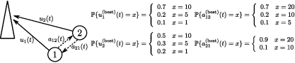
Simulation under the proposed quadratic policy and the standard max-weight policy is performed over a small network in Fig. 2. The network contains two devicess, 𝒩={1,2}{\mathcal{N}}=\{1,2\}. Each device has the other as its neighbor, so ℋ1={2}{\mathcal{H}}_{1}=\{2\} and ℋ2={1}{\mathcal{H}}_{2}=\{1\}. An event occurs in every slot with probability θ=0.3\theta=0.3. We assume all uplink and relay channels are orthogonal. The uplink channel distribution for device 11 is better than that of device 22 as in Fig. 2.

Refer to caption
Fig. 2: Small network with independent channels with distributions shown.

The constraints are un​(t)∈{0,…,un(best)​(𝜼⁡(t))}u_{n}(t)\in\{0,\ldots,u_{n}^{(\text{best})}({\boldsymbol{\eta}}(t))\} for n∈𝒩n\in{\mathcal{N}}. Also, a12​(t)∈{0,…,a12(best)​(𝜼⁡(t))}a_{12}(t)\in\{0,\ldots,a_{12}^{(\text{best})}({\boldsymbol{\eta}}(t))\} and a21​(t)∈{0,…,a21(best)​(𝜼⁡(t))}a_{21}(t)\in\{0,\ldots,a_{21}^{(\text{best})}({\boldsymbol{\eta}}(t))\}. Then set sn(q)​(max)=sn(j)​(max)=30s_{n}^{(q){(\text{max})}}=s_{n}^{(j){(\text{max})}}=30. The feasible set of formats is ℱ={0,1,2,3}{\mathcal{F}}=\{0,1,2,3\} with constant options given by (dn(0),rn(0))=(0,0),(dn(1),rn(1))=(100,20),(dn(2),rn(2))=(50,15),(dn(3),rn(3))=(10,10)(d_{n}^{(0)},r_{n}^{(0)})=(0,0),(d_{n}^{(1)},r_{n}^{(1)})=(100,20),(d_{n}^{(2)},r_{n}^{(2)})=(50,15),(d_{n}^{(3)},r_{n}^{(3)})=(10,10) whenever there is an event.

The simulation is performed according to the algorithm in Sec. III-C. The time-averaged quality of information under the quadratic and max-weight policies are shown in Fig. 3. From the plot, the values of y¯0\bar{y}_{0} under both policies converge to optimality following the O⁡(1/V)O(1/V) performance bound.

Refer to caption
Fig. 3: Quality of Information versus VV under the quadratic (QD) and max-weight (MW) policies

Fig. 4abc reveals queue lengths in the input, uplink, and relay queues of device 1 under the quadratic and max-weight policies. At the same VV, the quadratic policy reduces queue lengths by a significant constant compared to the cases under the max-weight policy. The plot also shows the growth of queue lengths with parameter VV, which follows the O⁡(V)O(V) bound of the queue length. Fig. 4d shows the average total queue length in device 1 under the quadratic and max-weight policies.

Fig. 5 shows that the quadratic policy can achieve near optimality with significantly smaller total system backlog compared to the case under the max-weight policy. This shows a significant advantage, which in turn affects memory size and packet delay.

Refer to caption
Fig. 4: Averaged backlog in queues versus VV and system quality versus backlog under the quadratic (QD) and max-weight (MW) policies
Refer to caption
Fig. 5: The system obtains average quality of information while having average total queue length

Another larger network shown in Fig. 6 is simulated to observe convergence of the proposed algorithm. As in the small network scenario, the same probability of event occurrence θ=0.3\theta=0.3 is set. Channel distributions are configured in Fig. 6. For V=800V=800, the time-averaged quality of information is 25.0025.00 after 10610^{6} time slots as shown in the upper plot of Fig. 7. The lower plot in Fig. 7 illustrates the early period of the simulation to illustrate convergence time.

Refer to caption
Fig. 6: Larger network with independent channels with distributions shown
Refer to caption
Fig. 7: Convergence of time-averaged quality of information. The interval of the moving average is 500 slots.

VI Linear Programs by Quadratic Policy

The generality of the quadratic policy is illustrated in this section. The policy is applied to solve linear programs which is one application of the Lyapunov optimization [12].

VI-A Problem Transformation

The following static linear program is considered where (xi)i=1n{\left({x_{i}}\right)}_{i=1}^{n} are decision variables and (aj​i)|j=1,i=1j=m,i=n{\left({a_{ji}}\right)}|_{j=1,i=1}^{j=m,i=n}, (bj)|j=1m{\left({b_{j}}\right)}|_{j=1}^{m}, (ci)|i=1n{\left({c_{i}}\right)}|_{i=1}^{n}, (xi(max))|i=1n{\left({x_{i}^{(\text{max})}}\right)}|_{i=1}^{n} are constants.

Maximize ∑i=1nci​xi\displaystyle\sum_{i=1}^{n}c_{i}x_{i} (57)
Subject to ∑i=1naj​i​xi≤bj,j∈{1,…,m}\displaystyle\sum_{i=1}^{n}a_{ji}x_{i}\leq b_{j},\quad\quad j\in{\left\{{1,\dotsc,m}\right\}}
0≤xi≤xi(max),i∈{1,…,n}\displaystyle 0\leq x_{i}\leq x_{i}^{(\text{max})},\quad\quad i\in\{1,\dotsc,n\}

In order to solve (57), the following time-averaged optimization problem is solved by using the Lyapunov optimization technique.

Maximize y¯0=∑i=1nci​x¯i\displaystyle\bar{y}_{0}=\sum_{i=1}^{n}c_{i}\bar{x}_{i} (58)
Subject to ∑i=1naj​i​x¯i≤bj,j∈{1,…,m}\displaystyle\sum_{i=1}^{n}a_{ji}\bar{x}_{i}\leq b_{j},\quad\quad j\in{\left\{{1,\dotsc,m}\right\}}
0≤xi​(t)≤xi(max),i∈{1,…,n},t≥0\displaystyle 0\leq x_{i}(t)\leq x_{i}^{(\text{max})},\quad\quad i\in{\left\{{1,\dotsc,n}\right\}},t\geq 0

Solutions from the static problem (57) and the time-averaged problem (58) are equivalent because using a solution xix_{i} to the static problem for every tt in the time-averaged problem leads to x¯i=xi\bar{x}_{i}=x_{i} for i∈{1,…,n}i\in{\left\{{1,\dotsc,n}\right\}} and every constraint in the time-averaged problem is satisfied. The time-averaged objective function is also maximized, since the time average of the linear function is equal to the function of the time averages. On the other hand, a solution to the time-averaged problem is a solution of the static problem because it satisfies all constraints and maximizes the same objective function.

To solve problem (58), a concept of virtual queue is used [12]. Let xi​(t)x_{i}(t) be chosen every slot tt in the interval 0≤xi​(t)≤xi(max)0\leq x_{i}(t)\leq x_{i}^{(\text{max})}, and define x¯i​(t)\bar{x}_{i}(t) for i∈{1,…,n}i\in{\left\{{1,\dotsc,n}\right\}} as

x¯i​(t)≜1t​∑τ=0t−1xi​(τ),i∈{1,…,n}.\bar{x}_{i}(t)\triangleq\frac{1}{t}\sum_{\tau=0}^{t-1}x_{i}(\tau),\quad i\in{\left\{{1,\dotsc,n}\right\}}.

Define virtual queue

Zj​(t+1)\displaystyle Z_{j}(t+1) =max⁡[Zj​(t)+∑i=1naj​i​xi​(t)−bj,0]\displaystyle=\max{\left[{Z_{j}(t)+\sum_{i=1}^{n}a_{ji}x_{i}(t)-b_{j},0}\right]} (59)

for all j∈{1,…,m}j\in{\left\{{1,\dotsc,m}\right\}}. It follows that

Zj​(τ+1)\displaystyle Z_{j}(\tau+1) =max⁡[Zj​(τ)+∑i=1naj​i​xi​(τ)−bj,0]\displaystyle=\max{\left[{Z_{j}(\tau)+\sum_{i=1}^{n}a_{ji}x_{i}(\tau)-b_{j},0}\right]}
≥Zj​(τ)+∑i=1naj​i​xi​(τ)−bj\displaystyle\geq Z_{j}(\tau)+\sum_{i=1}^{n}a_{ji}x_{i}(\tau)-b_{j}
Zj​(τ+1)−Zj​(τ)\displaystyle Z_{j}(\tau+1)-Z_{j}(\tau) ≥∑i=1naj​i​xi​(τ)−bj.\displaystyle\geq\sum_{i=1}^{n}a_{ji}x_{i}(\tau)-b_{j}.

Summing from τ=0\tau=0 to t−1t-1, and dividing by tt:

Zj​(t)−Zj​(0)\displaystyle Z_{j}(t)-Z_{j}(0) ≥∑τ=0t−1∑i=1naj​i​xi​(τ)−t​bj\displaystyle\geq\sum_{\tau=0}^{t-1}\sum_{i=1}^{n}a_{ji}x_{i}(\tau)-tb_{j}
Zj​(t)t\displaystyle\frac{Z_{j}(t)}{t} ≥1t​∑τ=0t−1∑i=1naj​i​xi​(τ)−bj\displaystyle\geq\frac{1}{t}\sum_{\tau=0}^{t-1}\sum_{i=1}^{n}a_{ji}x_{i}(\tau)-b_{j}
=∑i=1naj​i​x¯i​(t)−bj,\displaystyle=\sum_{i=1}^{n}a_{ji}\bar{x}_{i}(t)-b_{j}, (60)

where we assume that Zj​(0)≥0Z_{j}(0)\geq 0. It follows that if Z⁡(t)t→0\frac{Z(t)}{t}\rightarrow 0 (so that each queue is “rate stable”), the desired time-average inequality constraint is satisfied.

Then let 𝚯⁡(t)=(Zj​(t))|j=1m{\boldsymbol{\Theta}}(t)={\left({Z_{j}(t)}\right)}|_{j=1}^{m} be a vector of all virtual queues and

y0​(t)=∑i=1nci​xi​(t)y_{0}(t)=\sum_{i=1}^{n}c_{i}x_{i}(t)

be the objective function whose time average is to be minimized according to the problem (58). Define a time-averaged objective value up to iteration tt by

y¯0​(t)\displaystyle\bar{y}_{0}(t) ≜1t​∑τ=0t−1y0​(τ).\displaystyle\triangleq\frac{1}{t}\sum_{\tau=0}^{t-1}y_{0}(\tau).

Similar to Sec. II-C, let y¯0≜limt→∞y¯0​(t)\bar{y}_{0}\triangleq\lim_{t\rightarrow\infty}\bar{y}_{0}(t) be and x¯i≜limt→∞x¯i​(t)\bar{x}_{i}\triangleq\lim_{t\rightarrow\infty}\bar{x}_{i}(t) be their asymptotic averages.

VI-B Lyapunov Optimization

To solve (58), the drift-plus-penalty for this problem is bounded by Lemma 1 as

L⁡(𝚯⁡(t+1))−L⁡(𝚯⁡(t))−V​y0​(t)\displaystyle L({\boldsymbol{\Theta}}(t+1))-L({\boldsymbol{\Theta}}(t))-Vy_{0}(t)
=12​∑j=1m{Zj2​(t+1)−Zj2​(t)−2​V​ci​xi​(t)}\displaystyle\textstyle\quad=\frac{1}{2}\sum_{j=1}^{m}{\left\{{Z_{j}^{2}(t+1)-Z_{j}^{2}(t)-2Vc_{i}x_{i}(t)}\right\}}
=12∑j=1m{max[Zj(t)+∑i=1naj​ixi(t)−bj,0]\displaystyle\textstyle\quad=\frac{1}{2}\sum_{j=1}^{m}\bigl\{\max{\left[{Z_{j}(t)+\sum_{i=1}^{n}a_{ji}x_{i}(t)-b_{j},0}\right]}
−Zj2(t)−2Vcixi(t)}\displaystyle\textstyle\quad\quad-Z_{j}^{2}(t)-2Vc_{i}x_{i}(t)\bigr\} (61)
≤12∑j=1m{∑i=1n[Zi(t)+aj​ixi(t)]2+[Zj(t)−bj]2\displaystyle\textstyle\quad\leq\frac{1}{2}\sum_{j=1}^{m}\bigl\{\sum_{i=1}^{n}{\left[{Z_{i}(t)+a_{ji}x_{i}(t)}\right]}^{2}+{\left[{Z_{j}(t)-b_{j}}\right]}^{2}
−(n+1)Zj2(t)−2Vcixi+Hj}\displaystyle\textstyle\quad\quad-(n+1)Z_{j}^{2}(t)-2Vc_{i}x_{i}+H_{j}\bigr\}
=12​∑i=1n{∑j=1m[Zj​(t)+aj​i​xi​(t)]2−2​V​ci​xi​(t)}\displaystyle\textstyle\quad=\frac{1}{2}\sum_{i=1}^{n}{\left\{{\sum_{j=1}^{m}{\left[{Z_{j}(t)+a_{ji}x_{i}(t)}\right]}^{2}-2Vc_{i}x_{i}(t)}\right\}}
+12∑j=1m{[Zj(t)−bj]2−(n+1)Zj2(t)+Hj},\displaystyle\textstyle\quad\quad+\frac{1}{2}\sum_{j=1}^{m}{\left\{{{\left[{Z_{j}(t)-b_{j}}\right]}^{2}-(n+1)Z_{j}^{2}(t)+H_{j}}\right\}}, (62)

where

Hj=2{∑i=1n∑i′=1i−1|aj​i||aj​i′|xi(max)xi′(max)+∑i=1n|aj​i||bj|xi(max)}H_{j}=2\bigl\{\mbox{$\sum_{i=1}^{n}\sum_{i^{\prime}=1}^{i-1}$}{\left|{a_{ji}}\right|}{\left|{a_{ji^{\prime}}}\right|}x_{i}^{(\text{max})}x_{i^{\prime}}^{(\text{max})}\\ +\mbox{$\sum_{i=1}^{n}$}{\left|{a_{ji}}\right|}{\left|{b_{j}}\right|}x_{i}^{(\text{max})}\bigr\}

for j∈{1,…,m}j\in{\left\{{1,\dotsc,m}\right\}}. From (62), the quadratic policy minimize the drift-plus-penalty every iteration, and this minimization is

Minimize ∑i=1n{∑j=1m[Zj​(t)+aj​i​xi​(t)]2−2​V​ci​xi​(t)}\displaystyle\textstyle\sum_{i=1}^{n}{\left\{{\sum_{j=1}^{m}{\left[{Z_{j}(t)+a_{ji}x_{i}(t)}\right]}^{2}-2Vc_{i}x_{i}(t)}\right\}} (63)
Subject to 0≤xi​(t)≤xi(max)i∈{1,…,n}.\displaystyle 0\leq x_{i}(t)\leq x_{i}^{(\text{max})}\quad\quad i\in{\left\{{1,\dotsc,n}\right\}}.

Again, because problem’s structure and the fully separable property of the quadratic policy, problem (63) can be solved separately for each xi​(t)x_{i}(t). A closed form solution of each xi​(t)x_{i}(t) for i∈{1,…,n}i\in{\left\{{1,\dotsc,n}\right\}} is

xi​(t)=max⁡[min⁡[ci​V−∑j=1maj​i​Zj​(t)∑j=1maj​i2,xi(max)],0].\displaystyle x_{i}(t)=\max{\left[{\min{\left[{\frac{c_{i}V-\sum_{j=1}^{m}a_{ji}Z_{j}(t)}{\sum_{j=1}^{m}a_{ji}^{2}},x_{i}^{(\text{max})}}\right]},0}\right]}.

VI-C Algorithm

An algorithm to solve problem (58), which also solves (57), is the following.

Algorithm 3 Linear programming by quadratic policy
Initialize {𝚯⁡(0)}=𝟎{\left\{{{\boldsymbol{\Theta}}(0)}\right\}}={\boldsymbol{0}}
t=0t=0
foreach iteration t≥0t\geq 0 do
   // Update decision variables
   foreach i∈{1,…,n}i\in{\left\{{1,\dotsc,n}\right\}} do
      xi​(t)=max⁡[min⁡[ci​V−∑j=1maj​i​Zj​(t)∑j=1maj​i2,xi(max)],0]\textstyle x_{i}(t)=\max{\left[{\min{\left[{\frac{c_{i}V-\sum_{j=1}^{m}a_{ji}Z_{j}(t)}{\sum_{j=1}^{m}a_{ji}^{2}},x_{i}^{(\text{max})}}\right]},0}\right]}
   end foreach
   // Update virtual queues
   foreach j∈{1,…,m}j\in{\left\{{1,\dotsc,m}\right\}} do
      Zj​(t+1)=max⁡[Zj​(t)+(∑i=1naj​i​xi​(t)−bj),0]\textstyle Z_{j}(t+1)=\max{\left[{Z_{j}(t)+{\left({\sum_{i=1}^{n}a_{ji}x_{i}(t)-b_{j}}\right)},0}\right]}
   end foreach
   t=t+1t=t+1
end foreach

VI-D Convergence Analysis

Since our policy chooses xi​(t)∈[0,x(max)]x_{i}(t)\in[0,x^{(\text{max})}] every slot to minimize the right-hand-side of (62), this right-hand-side is less than or equal to the corresponding value with any other feasible decision xi∗∈[0,x(max)]x_{i}^{\ast}\in[0,x^{(\text{max})}]:

L⁡(𝚯⁡(τ+1))−L⁡(𝚯⁡(τ))−V​y0​(τ)\displaystyle L({\boldsymbol{\Theta}}(\tau+1))-L({\boldsymbol{\Theta}}(\tau))-Vy_{0}(\tau)
≤12​∑i=1n{∑j=1m[Zj​(t)+aj​i​xi∗​(t)]2−2​V​ci​xi∗​(t)}\displaystyle\textstyle\leq\frac{1}{2}\sum_{i=1}^{n}{\left\{{\sum_{j=1}^{m}{\left[{Z_{j}(t)+a_{ji}x_{i}^{\ast}(t)}\right]}^{2}-2Vc_{i}x_{i}^{\ast}(t)}\right\}}
+12∑j=1m{[Zj(t)−bj]2−(n+1)Zj2(t)+Hj}\displaystyle\textstyle\quad+\frac{1}{2}\sum_{j=1}^{m}{\left\{{{\left[{Z_{j}(t)-b_{j}}\right]}^{2}-(n+1)Z_{j}^{2}(t)+H_{j}}\right\}}
≤∑j=1mZj​(τ)​[∑i=1naj​i​xi∗​(τ)−bj]−V​∑i=1nci​xi∗​(τ)+E\displaystyle\textstyle\leq\sum_{j=1}^{m}Z_{j}(\tau){\left[{\sum_{i=1}^{n}a_{ji}x_{i}^{\ast}(\tau)-b_{j}}\right]}-V\sum_{i=1}^{n}c_{i}x_{i}^{\ast}(\tau)+E (64)

where

E=∑j=1m[∑i=1n|aj​i|​xi(max)+bj]2\displaystyle E=\sum_{j=1}^{m}{\left[{\sum_{i=1}^{n}{\left|{a_{ji}}\right|}x_{i}^{(\text{max})}+b_{j}}\right]}^{2}

and the final inequality uses (13).

Assume that problem (57) has 𝒙∗=(xi∗)|i=1n{\boldsymbol{x}}^{\ast}={\left({x_{i}^{\ast}}\right)}|_{i=1}^{n} as an optimal solution and y0(opt)y_{0}^{(\text{opt})} as the optimal cost. This optimal solution has the following properties:

y0(opt)\displaystyle y_{0}^{(\text{opt})} =∑i=1nci​xi∗\displaystyle=\sum_{i=1}^{n}c_{i}x_{i}^{\ast}
∑i=1naj​i​xi∗\displaystyle\sum_{i=1}^{n}a_{ji}x_{i}^{\ast} ≤bj,j∈{1,…,m}.\displaystyle\leq b_{j},\quad\quad j\in{\left\{{1,\dotsc,m}\right\}}.

By applying xi​(t)=xi∗x_{i}(t)=x_{i}^{\ast} every iteration, the bound (64) becomes

L⁡(𝚯⁡(τ+1))−L⁡(𝚯⁡(τ))−V​y0​(τ)\displaystyle L({\boldsymbol{\Theta}}(\tau+1))-L({\boldsymbol{\Theta}}(\tau))-Vy_{0}(\tau)
≤−V​y0(opt)+E\displaystyle\quad\leq-Vy_{0}^{(\text{opt})}+E

Summing from τ=0\tau=0 to t−1t-1 and rearranging lead to

L⁡(𝚯⁡(t))−L⁡(𝚯⁡(0))−V​∑τ=0t−1y0​(τ)\displaystyle L({\boldsymbol{\Theta}}(t))-L({\boldsymbol{\Theta}}(0))-V\sum_{\tau=0}^{t-1}y_{0}(\tau) ≤E​t−V​t​y0(opt)\displaystyle\leq Et-Vty_{0}^{(\text{opt})}

and

∑τ=0t−1y0​(τ)≥L⁡(𝚯⁡(t))−L⁡(𝚯⁡(0))−E​tV+t​y0(opt).\sum_{\tau=0}^{t-1}y_{0}(\tau)\geq\frac{L({\boldsymbol{\Theta}}(t))-L({\boldsymbol{\Theta}}(0))-Et}{V}+ty_{0}^{(\text{opt})}.

Since Algorithm 3 initializes 𝚯⁡(0)=𝟎{\boldsymbol{\Theta}}(0)={\boldsymbol{0}}, L⁡(𝚯⁡(0))=0L({\boldsymbol{\Theta}}(0))=0 and also L⁡(𝚯⁡(t))≥0L({\boldsymbol{\Theta}}(t))\geq 0. Then, dividing by tt leads to

1t​∑τ=0t−1y0​(τ)\displaystyle\frac{1}{t}\sum_{\tau=0}^{t-1}y_{0}(\tau) ≥L⁡(𝚯⁡(t))t​V−EV+y0(opt)\displaystyle\geq\frac{L({\boldsymbol{\Theta}}(t))}{tV}-\frac{E}{V}+y_{0}^{(\text{opt})} (65)
1t​∑τ=0t−1y0​(τ)\displaystyle\frac{1}{t}\sum_{\tau=0}^{t-1}y_{0}(\tau) ≥−EV+y0(opt).\displaystyle\geq-\frac{E}{V}+y_{0}^{(\text{opt})}. (66)

The bound (66) shows that, when VV is large, the time-averaged objective value from the algorithm approaches the optimal objective value.

Since the feasible set of (xi​(t))i=1n{\left({x_{i}(t)}\right)}_{i=1}^{n} in problem (58) is bounded, there exist some y0(max)≥0y_{0}^{(\text{max})}\geq 0 such that y0​(t)≤y0(max)y_{0}(t)\leq y_{0}^{(\text{max})} for all tt. Then, the bound (65) can also be rearranged to be

L⁡(𝚯⁡(t))\displaystyle L({\boldsymbol{\Theta}}(t)) ≤E​t+V​∑τ=0t−1y0​(τ)−V​t​y0(opt)\displaystyle\leq Et+V\sum_{\tau=0}^{t-1}y_{0}(\tau)-Vty_{0}^{(\text{opt})}
∑j=1mZj2​(t)\displaystyle\sum_{j=1}^{m}Z_{j}^{2}(t) ≤2​E​t+2​V​t​[y0(max)−y0(opt)]\displaystyle\leq 2Et+2Vt{\left[{y_{0}^{(\text{max})}-y_{0}^{(\text{opt})}}\right]}
Zj​(t)\displaystyle Z_{j}(t) ≤2​E​t+2​V​t​[y0(max)−y0(opt)]\displaystyle\leq\sqrt{2Et+2Vt{\left[{y_{0}^{(\text{max})}-y_{0}^{(\text{opt})}}\right]}}
Zj​(t)t\displaystyle\frac{Z_{j}(t)}{t} ≤1t​{2​E+2​V​[y0(max)−y0(opt)]}.\displaystyle\leq\sqrt{\frac{1}{t}{\left\{{2E+2V{\left[{y_{0}^{(\text{max})}-y_{0}^{(\text{opt})}}\right]}}\right\}}}.

From (60), it follows that

∑i=1naj​i​x¯i​(t)−bj≤1t​{2​E+2​V​[y0(max)−y0(opt)]}.\sum_{i=1}^{n}a_{ji}\bar{x}_{i}(t)-b_{j}\leq\sqrt{\frac{1}{t}{\left\{{2E+2V{\left[{y_{0}^{(\text{max})}-y_{0}^{(\text{opt})}}\right]}}\right\}}}. (67)

The bound (67) shows that the constraints of problem (57) are asymptotically satisfied as tt approaches infinity.

When the number of iterations is limited, we can obtain convergence results in this case by assuming V=1/εV=1/\varepsilon and t=1/ε3t=1/\varepsilon^{3} and consider (66) and (67). This leads to

y0(opt)−1t​∑τ=0t−1y0​(τ)≤E​ε=O⁡(ε).\displaystyle y_{0}^{(\text{opt})}-\frac{1}{t}\sum_{\tau=0}^{t-1}y_{0}(\tau)\leq E\varepsilon=O(\varepsilon).

and

∑i=1naj​i​x¯i​(t)−bj\displaystyle\sum_{i=1}^{n}a_{ji}\bar{x}_{i}(t)-b_{j} ≤11/ε3​{2​E+2/ε×[y0(max)−y0(opt)]}\displaystyle\leq\sqrt{\frac{1}{1/\varepsilon^{3}}{\left\{{2E+2/\varepsilon\times{\left[{y_{0}^{(\text{max})}-y_{0}^{(\text{opt})}}\right]}}\right\}}}
=O⁡(ε).\displaystyle=O(\varepsilon). (68)

Therefore, using O⁡(1/ε3)O(1/\varepsilon^{3}) iterations ensures the time-averaged value of y¯0​(t)\bar{y}_{0}(t) is within O⁡(ε)O(\varepsilon) of the optimal value y0(opt)y_{0}^{(\text{opt})}, and all constraints are within O⁡(ε)O(\varepsilon) of being satisfied. However, This O⁡(1/ε3)O(1/\varepsilon^{3}) tradeoff can be improved to an O⁡(1/ε2)O(1/\varepsilon^{2}) tradeoff if the problem (58) satisfies a mild “Slater assumption” as the following.

Assumption 2

There are values ϵ>0\epsilon>0 and y0(opt)≤y0(ϵ)≤y0(max)y_{0}^{(\text{opt})}\leq y_{0}^{(\epsilon)}\leq y_{0}^{(\text{max})} and a static policy choosing (xi∗)i=1n(x_{i}^{\ast})_{i=1}^{n} every iteration that satisfies:

y0∗​(t)\displaystyle\textstyle y_{0}^{\ast}(t) =y0(ϵ)\displaystyle=y_{0}^{(\epsilon)}
∑i=1naj​i​xi∗−bj\displaystyle\textstyle\sum_{i=1}^{n}a_{ji}x_{i}^{\ast}-b_{j} ≤−ϵj∈{1,…,m}\displaystyle\leq-\epsilon\quad\quad j\in{\left\{{1,\dotsc,m}\right\}}
0≤xi∗\displaystyle\textstyle 0\leq x_{i}^{\ast} ≤xi(max).\displaystyle\leq x_{i}^{(\text{max})}.

In fact, this assumption is a static version of Assumption 1 and is similar to a general Slater condition in the convex optimization theory [17].

Applying Assumption (2) to (64), it follows that

L⁡(𝚯⁡(τ+1))−L⁡(𝚯⁡(τ))−V​y0​(τ)\displaystyle L({\boldsymbol{\Theta}}(\tau+1))-L({\boldsymbol{\Theta}}(\tau))-Vy_{0}(\tau)
≤−V∑i=1ncixi∗+∑j=1mZj(τ)[∑i=1naj​ixi∗−bj]+E\displaystyle\textstyle\quad\leq-V\sum_{i=1}^{n}c_{i}x_{i}^{\ast}+\sum_{j=1}^{m}Z_{j}(\tau){\left[{\sum_{i=1}^{n}a_{ji}x_{i}^{\ast}-b_{j}}\right]}+E
≤−V​y0(ϵ)−ϵ​∑j=1mZj​(τ)+E\displaystyle\textstyle\quad\leq-Vy_{0}^{(\epsilon)}-\epsilon\sum_{j=1}^{m}Z_{j}(\tau)+E

From triangle inequality, ∥𝒁⁡(τ)∥≤∑j=1mZj\lVert{\boldsymbol{Z}}(\tau)\rVert\leq\sum_{j=1}^{m}Z_{j}, the above inequality is

L⁡(𝚯⁡(τ+1))−L⁡(𝚯⁡(τ))−V​y0​(τ)\displaystyle L({\boldsymbol{\Theta}}(\tau+1))-L({\boldsymbol{\Theta}}(\tau))-Vy_{0}(\tau)
≤−V​y0(ϵ)−ϵ⁡∥𝒁⁡(τ)∥+E\displaystyle\textstyle\quad\leq-Vy_{0}^{(\epsilon)}-\epsilon\lVert{\boldsymbol{Z}}(\tau)\rVert+E

Since L⁡(𝚯⁡(τ))=12​∥𝒁⁡(τ)∥2L({\boldsymbol{\Theta}}(\tau))=\frac{1}{2}\lVert{\boldsymbol{Z}}(\tau)\rVert^{2}, we have:

∥𝒁⁡(τ+1)∥2−∥𝒁⁡(τ)∥2≤2​[V⁡(y0​(τ)−y0(ϵ))−ϵ⁡∥𝒁⁡(τ)∥+E].\displaystyle\lVert{\boldsymbol{Z}}(\tau+1)\rVert^{2}-\lVert{\boldsymbol{Z}}(\tau)\rVert^{2}\leq 2{\left[{V{\left({y_{0}(\tau)-y_{0}^{(\epsilon)}}\right)}-\epsilon\lVert{\boldsymbol{Z}}(\tau)\rVert+E}\right]}.

If ∥𝒁⁡(τ)∥≥V⁡(y0(max)−y0(ϵ))+Eϵ\lVert{\boldsymbol{Z}}(\tau)\rVert\geq\frac{V{\left({y_{0}^{(\text{max})}-y_{0}^{(\epsilon)}}\right)}+E}{\epsilon}, then

∥𝒁⁡(τ+1)∥2−∥𝒁⁡(τ)∥2\displaystyle\lVert{\boldsymbol{Z}}(\tau+1)\rVert^{2}-\lVert{\boldsymbol{Z}}(\tau)\rVert^{2} ≤0.\displaystyle\leq 0.

Since ∑j=1mZj2​(τ)=∥𝒁⁡(τ)∥2\sum_{j=1}^{m}Z_{j}^{2}(\tau)=\lVert{\boldsymbol{Z}}(\tau)\rVert^{2}, the above inequality implies that the value of ∑j=1mZj2​(τ)\sum_{j=1}^{m}Z_{j}^{2}(\tau) is not increased in the next iteration. Therefore, the value of each Zj​(τ)Z_{j}(\tau) is bounded by, for all τ≥0\tau\geq 0,

Zj​(τ)≤V⁡(y0(max)−y0(ϵ))+Eϵ+∑i=1n|aj​i|​xi(max).Z_{j}(\tau)\leq\frac{V{\left({y_{0}^{(\text{max})}-y_{0}^{(\epsilon)}}\right)}+E}{\epsilon}+\sum_{i=1}^{n}|a_{ji}|x_{i}^{(\text{max})}.

Dividing by τ\tau:

Zj​(τ)τ≤V⁡(y0(max)−y0(ϵ))+Eϵ​τ+∑i=1n|aj​i|​xi(max)τ.\frac{Z_{j}(\tau)}{\tau}\leq\frac{V{\left({y_{0}^{(\text{max})}-y_{0}^{(\epsilon)}}\right)}+E}{\epsilon\tau}+\frac{\sum_{i=1}^{n}|a_{ji}|x_{i}^{(\text{max})}}{\tau}.

When V=1/εV=1/\varepsilon and τ=1/ε2\tau=1/\varepsilon^{2}, it follows that

Zj​(τ)τ\displaystyle\frac{Z_{j}(\tau)}{\tau} ≤1/ε×(y0(max)−y0(ϵ))+Eϵ/ε2+∑i=1n|aj​i|​xi(max)1/ε2\displaystyle\leq\frac{1/\varepsilon\times{\left({y_{0}^{(\text{max})}-y_{0}^{(\epsilon)}}\right)}+E}{\epsilon/\varepsilon^{2}}+\frac{\sum_{i=1}^{n}|a_{ji}|x_{i}^{(\text{max})}}{1/\varepsilon^{2}}
=O⁡(ε).\displaystyle=O(\varepsilon).

From (60), it follows that

∑i=1naj​i​x¯i​(t)−bj≤O⁡(ε).\sum_{i=1}^{n}a_{ji}\bar{x}_{i}(t)-b_{j}\leq O(\varepsilon).

Thus, under Assumption 2, using O⁡(1/ε2)O(1/\varepsilon^{2}) iterations ensures the time-averaged value of y¯0​(t)\bar{y}_{0}(t) is within O⁡(ε)O(\varepsilon) of the optimal value y0(opt)y_{0}^{(\text{opt})}, and all constraints are within O⁡(ε)O(\varepsilon) of being satisfied. This is the O⁡(1/ε2)O(1/\varepsilon^{2}) tradeoff between computation and accuracy.

VI-E Example

For an example, we solved a small linear programming problem by using the max-weight and quadratic policies. The problem is

Maximize 2​x1+x2\displaystyle 2x_{1}+~x_{2}
Subject to x1+x2≤4\displaystyle~x_{1}+~x_{2}\leq 4
5​x1+3​x2≤15\displaystyle 5x_{1}+3x_{2}\leq 15
x1≤2.5\displaystyle~x_{1}\quad\quad\leq 2.5
0≤x1≤10\displaystyle 0\leq x_{1}\leq 10
0≤x2≤10.\displaystyle 0\leq x_{2}\leq 10.

The solution of this problem is x1=2.5,x2=0.833x_{1}=2.5,x_{2}=0.833. For both policies, the parameters are V=200V=200 and the number of iteration is 500500. The values of decision variables xi​(t)x_{i}(t) from both policies are shown in figure 8. The numerical values are show in table I.

TABLE I: Numerical results from an example problem
Quadratic Max-weight Optimal
x¯1​(500)\bar{x}_{1}(500) 2.5312.531 2.5402.540 2.5002.500
x¯2​(500)\bar{x}_{2}(500) 0.8340.834 0.8200.820 0.8330.833
x1​(500)x_{1}(500) 2.5002.500 0.0000.000 2.5002.500
x2​(500)x_{2}(500) 0.8330.833 0.0000.000 0.8330.833

These time-averaged values of decision variables from both policies approach the optimal solution. If number of iteration is increased, the precision is increased. Interestingly, the quadratic policy has a smooth property, as shown in Fig. 8, and that the intermediate decision values converge to an optimal solution before the time-averaged values does.

Refer to caption
Fig. 8: Comparison between max-weight and quadratic policies for solving linear programming

VII Conclusion

We studied information quality maximization in a system with uplink and single-hop relay capability which was done by designing queuing dynamic. From Lyapunov optimization theory, we proposed a novel quadratic policy having a separable property, which leads to a distributed mechanism of format selection. In comparison with the standard method, max-weight policy, our policy leads to an algorithm that reduces queue backlog by a significant constant. This reduction also propagates and grows with the number of queues in the system. We simulated the algorithm to verify correctness and behavior of the new policy. In addition, we shows how the novel policy is applied to solve linear programs.

References

  • [1] S. Supittayapornpong and M. J. Neely, “Quality of information maximization in two-hop wireless networks,” in IEEE ICC, 2012.
  • [2] E. Miluzzo, N. D. Lane, K. Fodor, R. Peterson, H. Lu, M. Musolesi, S. B. Eisenman, X. Zheng, and A. T. Campbell, “Sensing meets mobile social networks: the design, implementation and evaluation of the cenceme application,” ser. SenSys ’08. ACM, 2008.
  • [3] S. Kang, J. Lee, H. Jang, Y. Lee, S. Park, and J. Song, “A scalable and energy-efficient context monitoring framework for mobile personal sensor networks,” Mobile Computing, IEEE Transactions on, May. 2010.
  • [4] M. Mun, S. Reddy, K. Shilton, N. Yau, J. Burke, D. Estrin, M. Hansen, E. Howard, R. West, and P. Boda, “PEIR, the personal environmental impact report, as a platform for participatory sensing systems research,” ser. MobiSys ’09. ACM, 2009.
  • [5] R. Y. Wang and D. M. Strong, “Beyond accuracy: what data quality means to data consumers,” J. Manage. Inf. Syst., Mar. 1996.
  • [6] M. E. Johnson and K. C. Chang, “Quality of information for data fusion in net centric publish and subscribe architectures,” in Int’l Conf. on Information Fusion, Jul. 2005.
  • [7] C. Bisdikian, L. M. Kaplan, M. B. Srivastava, D. J. Thornley, D. Verma, and R. I. Young, “Building principles for a quality of information specification for sensor information,” Int’l Conf. on Information Fusion, Jul. 2009.
  • [8] C. H. Liu, C. Bisdikian, J. W. Branch, and K. K. Leung, “Qoi-aware wireless sensor network management for dynamic multi-task operations,” in Sensor Mesh and Ad Hoc Communications and Networks (SECON), Jul. 2010.
  • [9] A. Bar-Noy, G. Cirincione, R. Govindan, S. Krishnamurthy, T. F. LaPorta, P. Mohapatra, M. J. Neely, and A. Yener, “Quality-of-information aware networking for tactical military networks,” in IEEE PERCOM Workshops, Mar. 2011.
  • [10] B. Liu, P. Terlecky, A. Bar-Noy, R. Govindan, and M. J. Neely, “Optimizing information credibility in social swarming applications,” in IEEE INFOCOM, Apr. 2011.
  • [11] M. J. Neely, Stochastic Network Optimization with Application to Communication and Queueing Systems. Morgan & Claypool, 2010.
  • [12] L. Georgiadis, M. J. Neely, and L. Tassiulas, “Resource allocation and cross-layer control in wireless networks,” Foundations and Trends in Networking, 2006.
  • [13] M. J. Neely, “Distributed and secure computation of convex programming over a network of connected processors,” DCDIS Conf., Guelph, Ontario, Jul. 2005.
  • [14] Y. Nesterov, “Primal-dual subgradient methods for convex problems,” Mathematical Programming, 2009.
  • [15] S. Boyd, N. Parikh, E. Chu, B. Peleato, and J. Eckstein, Distributed Optimization and Statistical Learning via the Alternating Direction Method of Multipliers. Foundations and Trends in Networking, 2010.
  • [16] L. Ying, S. Shakkottai, A. Reddy, and S. Liu, “On combining shortest-path and back-pressure routing over multihop wireless networks,” IEEE/ACM Transactions on Networking, vol. vol. 19, no. 3, pp. 841-854, Jun. 2011.
  • [17] D. P. Bertsekas, A. Nedic, and A. E. Ozdaglar, Convex Analysis and Optimization. Athena Scientific, 2003.