跳到论文正文
W Papers独立论文阅读器 arXiv:1211.6045 论文正文 计算阅读时间 · 0%
引用这篇论文根据当前论文元数据生成,正式投稿前建议核对。


License: arXiv.org perpetual non-exclusive license
arXiv:1211.6045v1 [nlin.CD] 26 Nov 2012

Non-integrability of flail triple pendulum

Maria Przybylska Affiliation: Institute of Physics, University of Zielona Góra, Affiliation: Licealna 9, PL-65–417, Zielona Góra, Poland Affiliation: e-mail: M.Przybylska@proton.if.uz.zgora.pl Affiliation: and Affiliation: Wojciech Szumiński Affiliation: Institute of Physics, University of Zielona Góra, Affiliation: Licealna 9, PL-65–417, Zielona Góra, Poland Affiliation: e-mail: uz88szuminski@gmail.com
Abstract

We consider a special type of triple pendulum with two pendula attached to end mass of another one. Although we consider this system in the absence of the gravity, a quick analysis of of Poincaré cross sections shows that it is not integrable. We give an analytic proof of this fact analysing properties the of differential Galois group of variational equation along certain particular solutions of the system.

AMS Subject Classification: 70H07; 70H12; 70F07

1 Introduction

In this paper we study dynamics of a special type of triple pendulum which we called a flail. It consists of three pendula. The first one is attached to a fixed point, and to its end mass the other two pendula are joined. The lengths and the masses of pendula are l1,l2,l3l_{1},l_{2},l_{3}, and m1,m2,m3m_{1},m_{2},m_{3}, respectively, see Fig. 1. We consider this system in the absence of gravity. Similar problem of dynamics of a simple triple pendulum in the absence of gravity field was analysed in [13].

Figure 1: Geometry of the flail pendulum

The configuration space of our system is a torus 𝕋3=𝕊1×𝕊1×𝕊1\mathbb{T}^{3}=\mathbb{S}^{1}\times\mathbb{S}^{1}\times\mathbb{S}^{1} with local coordinates (θ1,θ2,θ3)mod2​π(\theta_{1},\theta_{2},\theta_{3})\mod 2\pi. We chose the point of suspension of the first pendulum as the origin, and angles are measured from vertical line as it is shown in Fig. 1. The Lagrange function has the following form

L=12​(l12​μ​θ˙12+l22​m2​θ˙22+l32​m3​θ˙32)+l1​l2​m2​cos⁡(θ1−θ2)​θ˙1​θ˙2+l1​l3​m3​cos⁡(θ1−θ3)​θ˙1​θ˙3,\begin{split}L&=\dfrac{1}{2}\left(l_{1}^{2}\mu\dot{\theta}_{1}^{2}+l_{2}^{2}m_{2}\dot{\theta}_{2}^{2}+l_{3}^{2}m_{3}\dot{\theta}_{3}^{2}\right)+l_{1}l_{2}m_{2}\cos(\theta_{1}-\theta_{2})\dot{\theta}_{1}\dot{\theta}_{2}\\ &+l_{1}l_{3}m_{3}\cos(\theta_{1}-\theta_{3})\dot{\theta}_{1}\dot{\theta}_{3},\end{split} (1.1)

where μ=m1+m2+m3\mu=m_{1}+m_{2}+m_{3}. Let us remark that the dynamics of this system can be interpreted as a geodesic motion on torus 𝕋3\mathbb{T}^{3}. The system has 𝕊1\mathbb{S}^{1} symmetry. This is why the Lagrange function depends on differences of angles only. Hence, it is reasonable to introduce new variables defined by

γ1=θ2−θ1,γ2=θ3−θ2,γ3=θ1\gamma_{1}=\theta_{2}-\theta_{1},\qquad\gamma_{2}=\theta_{3}-\theta_{2},\qquad\gamma_{3}=\theta_{1} (1.2)

and corresponding momenta

π1=(l22m2+l32m3)γ˙1+l32m3γ˙2+[l22m2+l32m3+l1l2m2cosγ1+l1l3m3cos(γ1+γ2)]γ˙3,π2=l32​m3​γ˙1+l32​m3​γ˙2+l3​m3​[l3+l1​cos⁡(γ1+γ2)]​γ˙3,π3=[l22m2+l32m3+l1l2m2cosγ1+l1l3m3cos(γ1+γ2)]γ˙1+l3m3[l3+l1cos(γ1+γ2)]γ˙2+[l22m2+l32m3+l12μ+2l1l2m2cosγ1+2l1l3m3cos(γ1+γ2)]γ˙3.\begin{split}&\pi_{1}=(l_{2}^{2}m_{2}+l_{3}^{2}m_{3})\dot{\gamma}_{1}+l_{3}^{2}m_{3}\dot{\gamma}_{2}+[l_{2}^{2}m_{2}+l_{3}^{2}m_{3}+l_{1}l_{2}m_{2}\cos\gamma_{1}+l_{1}l_{3}m_{3}\cos(\gamma_{1}+\gamma_{2})]\dot{\gamma}_{3},\\ &\pi_{2}=l_{3}^{2}m_{3}\dot{\gamma}_{1}+l_{3}^{2}m_{3}\dot{\gamma}_{2}+l_{3}m_{3}[l_{3}+l_{1}\cos(\gamma_{1}+\gamma_{2})]\dot{\gamma}_{3},\\ &\pi_{3}=[l_{2}^{2}m_{2}+l_{3}^{2}m_{3}+l_{1}l_{2}m_{2}\cos\gamma_{1}+l_{1}l_{3}m_{3}\cos(\gamma_{1}+\gamma_{2})]\dot{\gamma}_{1}+l_{3}m_{3}[l_{3}+l_{1}\cos(\gamma_{1}+\gamma_{2})]\dot{\gamma}_{2}\\ &+[l_{2}^{2}m_{2}+l_{3}^{2}m_{3}+l_{1}^{2}\mu+2l_{1}l_{2}m_{2}\cos\gamma_{1}+2l_{1}l_{3}m_{3}\cos(\gamma_{1}+\gamma_{2})]\dot{\gamma}_{3}.\end{split}

Now, γ3\gamma_{3} is a cyclic variable, and π3\pi_{3} is a first integral. Thus, after this reduction, the system has two degrees of freedom and its dynamics is determined by Hamiltonian

H=[l12μ(l32m3(π1−π2)2+l22m2π22)+l22l32m2m3(π1−c)2−l1(l1l22m22π22cosγ12+l3m3cos(γ1+γ2)(2l22m2π2(c−π1)+l1l3m3(π1−π2)2cos(γ1+γ2))−2l2l3m2m3(π1−π2)cosγ1(l3(π1−c)+l1π2cos(γ1+γ2)))]/[2l12l22l32m2m3B],\begin{split}H&=[l_{1}^{2}\mu(l_{3}^{2}m_{3}(\pi_{1}-\pi_{2})^{2}+l_{2}^{2}m_{2}\pi_{2}^{2})+l_{2}^{2}l_{3}^{2}m_{2}m_{3}(\pi_{1}-c)^{2}\\ &-l_{1}(l_{1}l_{2}^{2}m_{2}^{2}\pi_{2}^{2}\cos\gamma_{1}^{2}+l_{3}m_{3}\cos(\gamma_{1}+\gamma_{2})(2l_{2}^{2}m_{2}\pi_{2}(c-\pi_{1})\\ &+l_{1}l_{3}m_{3}(\pi_{1}-\pi_{2})^{2}\cos(\gamma_{1}+\gamma_{2}))-2l_{2}l_{3}m_{2}m_{3}(\pi_{1}-\pi_{2})\cos\gamma_{1}(l_{3}(\pi_{1}-c)\\ &+l_{1}\pi_{2}\cos(\gamma_{1}+\gamma_{2})))]/[2l_{1}^{2}l_{2}^{2}l_{3}^{2}m_{2}m_{3}B],\end{split} (1.3)

where

B:=μ−m2​cos2⁡γ1−m3​cos2⁡(γ1+γ2),B:=\mu-m_{2}\cos^{2}\gamma_{1}-m_{3}\cos^{2}(\gamma_{1}+\gamma_{2}),

and c:=π3c:=\pi_{3} is a parameter.

Refer to caption
Refer to caption
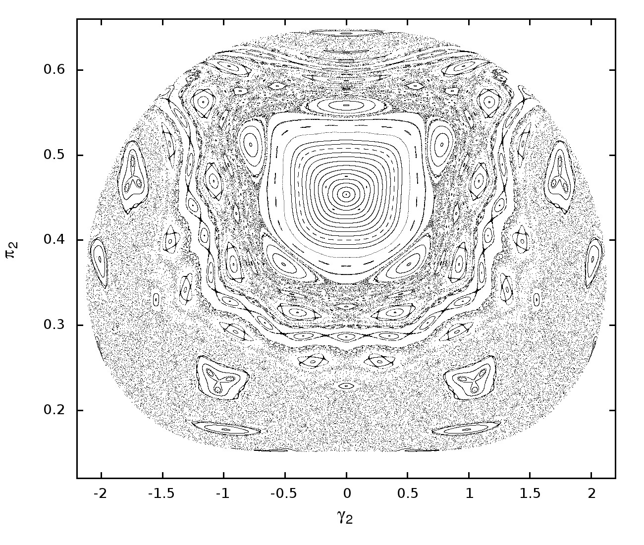
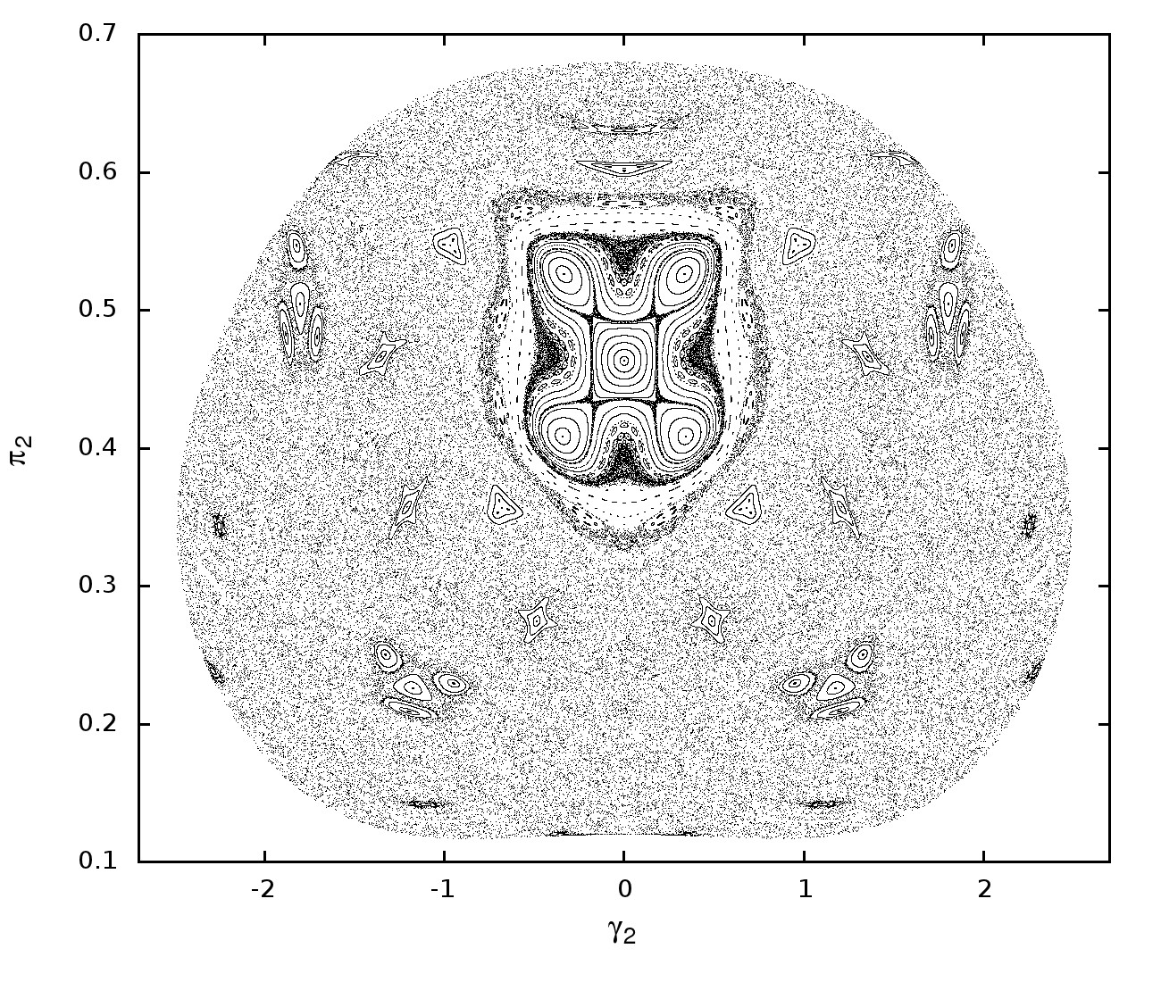
Figure 2: The Poincaré sections for E=0.01E=0.01 (on the left) and E=0.01005E=0.01005 (on the right)
Refer to caption
Refer to caption
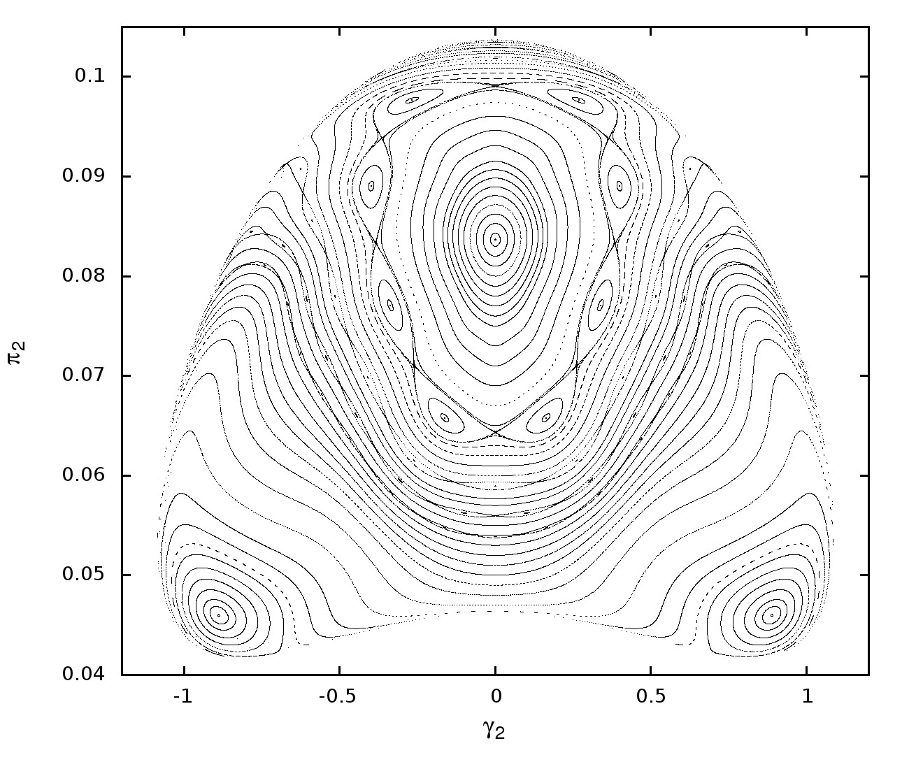
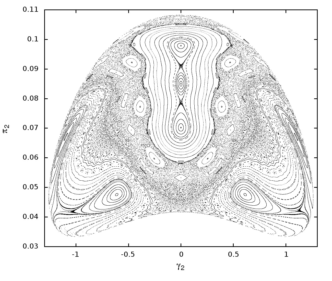
Figure 3: The Poincaré sections for E=0.0102E=0.0102 (on the left) and E=0.011E=0.011 (on the right)
Refer to caption
Refer to caption
Figure 4: The Poincaré sections for E=0.012E=0.012 (on the left) and E=0.013E=0.013 (on the right)

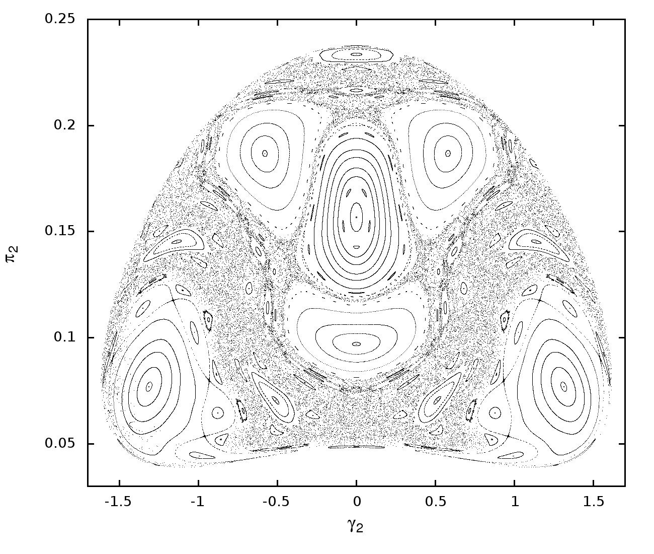
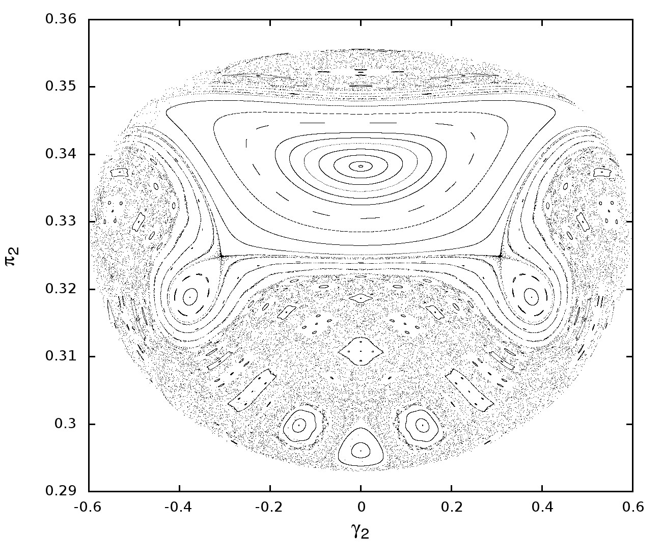
The aim of this paper is an analysis of integrability of this reduced system. To get an idea about the complexity of dynamics we made several Poincaré cross sections. In Figures 2, 3, and 4 we show such cross sections. We take γ1=0\gamma_{1}=0 and π1>0\pi_{1}>0 as the cross section plane. The phase portraits are presented in (γ2,y2)(\gamma_{2},y_{2}) plane. The cross sections are made for the following values of parameters:

π3=c=1,m1=1,m2=3,m3=2,l1=1,l2=2,l3=3.\pi_{3}=c=1,\quad m_{1}=1,\quad m_{2}=3,\quad m_{3}=2,\quad l_{1}=1,\quad l_{2}=2,\quad l_{3}=3. (1.4)

Figures are ordered according to increasing energy of the system. They show that, for chosen values of parameters, the system is not integrable. The main problem considered in this paper is to prove that for a wide range of the parameters the system is in fact non-integrable. Our main result we formulate in the following theorem.

Theorem 1.1.

If the reduced flail system governed by Hamiltonian (1.3) has parameters satisfying

  • •

    m1≠0m_{1}\neq 0, c≠0c\neq 0, l2≠l3l_{2}\neq l_{3}, and m2​l2=m3​l3m_{2}l_{2}=m_{3}l_{3}; or

  • •

    m2=m3m_{2}=m_{3}, l2=l3l_{2}=l_{3}, and c=0c=0,

then it is nonintegrable in the class of meromorphic functions of coordinates and momenta.

The plan of the paper is the following. Section 2 contains the non-integrability proof and is divided into two subsections. In Section 3 some remarks are given. Explicit forms of some complicated expressions are given in Appendix A. For convenience of readers in Appendix B basic information about linear second order differential equation with rational coefficients and Kovacic algorithm are given.

2 Non-integrability proof

In this section we prove Theorem 1.1 using the Morales-Ramis theory, see [1, 11].

We formulate the main theorem of this theory in the following simple settings. Let us consider a complex Hamiltonian system. We assume that the underlying phase space is ℂ2​n\mathbb{C}^{2n}, which is considered as a linear symplectic space equipped with the canonical symplectic form

ω=∑i=1nd​qi∧d​pi,\omega=\sum_{i=1}^{n}\mathrm{d}q_{i}\wedge\mathrm{d}p_{i},

where 𝒙=(q1,…,qn,p1,…,pn)\boldsymbol{x}=(q_{1},\ldots,q_{n},p_{1},\ldots,p_{n}) are the canonical coordinates. Let H:ℂ2​n→ℂH:\mathbb{C}^{2n}\rightarrow\mathbb{C} be a holomorphic Hamiltonian, and

dd​t​𝒙=𝒗H​(𝒙),𝒗H​(x)=𝕀2​n​∇𝒙H,𝒙∈ℂ2​n,t∈ℂ,\frac{\mathrm{d}\phantom{t}}{\mathrm{d}\mspace{1mu}t}\boldsymbol{x}=\boldsymbol{v}_{H}(\boldsymbol{x}),\quad\boldsymbol{v}_{H}(x)=\mathbb{I}_{2n}\nabla_{\boldsymbol{x}}H,\qquad\boldsymbol{x}\in\mathbb{C}^{2n},\quad t\in\mathbb{C}, (2.1)

the associated Hamilton equations. Here 𝕀2​n\mathbb{I}_{2n} denotes 2​n×2​n2n\times 2n symplectic unit matrix.

Let t↦𝝋⁡(t)∈ℂ2​nt\mapsto\boldsymbol{\varphi}(t)\in\mathbb{C}^{2n} be a non-equilibrium solution of (2.1). The maximal analytic continuation of 𝝋⁡(t)\boldsymbol{\varphi}(t) defines a Riemann surface 𝚪\boldsymbol{\Gamma} with tt as a local coordinate. Variational equations along 𝝋⁡(t)\boldsymbol{\varphi}(t) have the form

dd​t​𝝃=𝑨⁡(t)​𝝃,𝑨⁡(t)=∂𝒗H∂𝒙​(𝝋⁡(t)).\frac{\mathrm{d}\phantom{t}}{\mathrm{d}\mspace{1mu}t}\boldsymbol{\xi}=\boldsymbol{A}(t)\boldsymbol{\xi},\qquad\boldsymbol{A}(t)=\dfrac{\partial\boldsymbol{v}_{H}}{\partial\boldsymbol{x}}(\boldsymbol{\varphi}(t)). (2.2)

We can attach to this equations the differential Galois group 𝒢{\mathcal{G}}. Roughly speaking, 𝒢{\mathcal{G}} is an algebraic subgroup of GL⁡(2​n,ℂ)\mathrm{GL}(2n,\mathbb{C}), which preserves polynomial relations between solutions of (2.2). As a linear algebraic group, among other things, it is a union of a finite number of disjoint connected components. One of them, containing the identity, is called the identity component of 𝒢{\mathcal{G}}, and is denoted by 𝒢0{\mathcal{G}}^{0}. For a precise definition of the differential Galois group and differential Galois theory see e.g., [5, 2, 10, 14]. It appears that the integrability of the considered system manifests itself in properties of the differential Galois group of the variational equations. For Hamiltonian system and integrability in the Liouville sense this relation is particularly elegant. For these systems 𝒢{\mathcal{G}} is an algebraic subgroup of Sp⁡(2​n,ℂ)\mathrm{Sp}(2n,\mathbb{C}). In nineties of XX century Morales-Ruiz and Ramis showed that the integrability in the Liouville sense imposes a very restrictive condition on 𝒢0{\mathcal{G}}^{0} [1, 12, 11].

Theorem 2.1 (Morales-Ruiz and Ramis).

Assume that a Hamiltonian system is meromorphically integrable in the Liouville sense in a neigbourhood of a phase curve 𝚪\boldsymbol{\Gamma}. Then the identity component of the differential Galois group of NVEs associated with 𝚪\boldsymbol{\Gamma} is Abelian.

In order to apply this theorem we need an effective method which allows to determine properties of the differential Galois group of linear equations. In the investigated system variational equations split into two subsystems of linear equations. Each of these subsystems can be transformed into equivalent second order equation with rational coefficients. For such equation there exists the Kovacic algorithm [7], see also Appendix B, which allows to determine the differential Galois group. We apply this algorithm in our considerations.

2.1 Case m2≠m3m_{2}\neq m_{3} and l2≠l3l_{2}\neq l_{3}

At first we make the following non-canonical transformation

[γ1γ2π1π2]=𝑨​[x1x2y1y2],𝑨=[01001−2000011−l2l30001].\begin{bmatrix}\gamma_{1}\\ \gamma_{2}\\ \pi_{1}\\ \pi_{2}\end{bmatrix}=\boldsymbol{A}\begin{bmatrix}x_{1}\\ x_{2}\\ y_{1}\\ y_{2}\end{bmatrix},\qquad\boldsymbol{A}=\begin{bmatrix}0&1&0&0\\ 1&-2&0&0\\ 0&0&1&1-\dfrac{l_{2}}{l_{3}}\\ 0&0&0&1\end{bmatrix}. (2.3)

After this transformation equations of motion take the form

𝒙˙=𝕁2​n​∇𝒙H~,𝒙=[x1,x2,y1,y2]T,\dot{\boldsymbol{x}}=\mathbb{J}_{2n}\nabla_{\boldsymbol{x}}\widetilde{H},\qquad\boldsymbol{x}=[x_{1},x_{2},y_{1},y_{2}]^{T}, (2.4)

where

𝕁2​n:=𝐁​𝕀​𝑩T,𝑩=𝑨−1,H~​(𝒙):=H⁡(𝑨​𝒙).\mathbb{J}_{2n}:={\mathbf{B}}\mathbb{I}\boldsymbol{B}^{T},\qquad\boldsymbol{B}=\boldsymbol{A}^{-1},\quad\widetilde{H}(\boldsymbol{x}):=H(\boldsymbol{A}\boldsymbol{x}). (2.5)

The explicit form of Hamiltonian in these variable is following

H~=[l22m2m3(cl3+l2y2−l3(y1+y2))2+l12μ(l22m2y22+m3(l3y1−l2y2)2)−l1​(m3​cos⁡(x1−x2)​(2​l22​m2​y2​(c​l3+l2​y2−l3​(y1+y2))+l1​m3​(l3​y1−l2​y2)2​cos⁡(x1−x2))CLOSE+2l2m2m3(−l3y1+l2y2)(−l2y2+l3(−c+y1+y2)+l1y2cos(x1−x2))cosx2+l1l22m22y22cosx22)]/[2l12l22l32m2m3(μ−m3cos(x1−x2)2−m2cosx22)].\begin{split}&\widetilde{H}=\left[l_{2}^{2}m_{2}m_{3}\left(cl_{3}+l_{2}y_{2}-l_{3}(y_{1}+y_{2})\right)^{2}+l_{1}^{2}\mu\left(l_{2}^{2}m_{2}y_{2}^{2}+m_{3}(l_{3}y_{1}-l_{2}y_{2})^{2}\right)\right.\\ &-l_{1}\left(m_{3}\cos(x_{1}-x_{2})\left(2l_{2}^{2}m_{2}y_{2}\left(cl_{3}+l_{2}y_{2}-l_{3}(y_{1}+y_{2})\right)+l_{1}m_{3}(l_{3}y_{1}-l_{2}y_{2})^{2}\cos(x_{1}-x_{2})\right)\right.\\ &+2l_{2}m_{2}m_{3}(-l_{3}y_{1}+l_{2}y_{2})\left(-l_{2}y_{2}+l_{3}(-c+y_{1}+y_{2})+l_{1}y_{2}\cos(x_{1}-x_{2})\right)\cos x_{2}\\ &+\left.\left.l_{1}l_{2}^{2}m_{2}^{2}y_{2}^{2}\cos x_{2}^{2}\right)\right]/[2l_{1}^{2}l_{2}^{2}l_{3}^{2}m_{2}m_{3}(\mu-m_{3}\cos(x_{1}-x_{2})^{2}-m_{2}\cos x_{2}^{2})].\end{split} (2.6)

An explicit form of vector field 𝒗⁡(𝒙):=𝕁2​n​∇𝒙H~\boldsymbol{v}(\boldsymbol{x}):=\mathbb{J}_{2n}\nabla_{\boldsymbol{x}}\widetilde{H} is given in Appendix A, see equation (A.1). These equations are still Hamiltonian but written in non-canonical variables.

Let us assume that the following conditions

m2​l2=m3​l3,l2≠l3,m_{2}l_{2}=m_{3}l_{3},\qquad l_{2}\neq l_{3}, (2.7)

are fulfilled. Then, system (2.4) has an invariant manifold

𝒩={(x1,x2,y1,y2)∈ℂ4|x1=y1=0,y2=−cl3/(l2−l3)}.{\mathcal{N}}=\{(x_{1},x_{2},y_{1},y_{2})\in\mathbb{C}^{4}\ |\ x_{1}=y_{1}=0,\,y_{2}=-cl_{3}/(l_{2}-l_{3})\}.

In fact, restricting the right hand sides of system (2.4) to 𝒩{\mathcal{N}}, and putting m3=m2​l2/l3m_{3}={m_{2}l_{2}}/{l_{3}}, we obtain

x˙1=0,x˙2=cl2​m2​(l2−l3),y˙1=0,y˙2=0.\dot{x}_{1}=0,\qquad\dot{x}_{2}=\dfrac{c}{l_{2}m_{2}(l_{2}-l_{3})},\qquad\dot{y}_{1}=0,\qquad\dot{y}_{2}=0. (2.8)

Hence, solving the above equations we obtain our particular solution ℂ∋t↦𝝋⁡(t)\mathbb{C}\ni t\mapsto\boldsymbol{\varphi}(t).

Let 𝑿:=[X1,X2,Y1,Y2]T\boldsymbol{X}:=[X_{1},X_{2},Y_{1},Y_{2}]^{T} denote variations of [x1,x2,y1,y2]T[x_{1},x_{2},y_{1},y_{2}]^{T}. The variational equations along 𝝋⁡(t)\boldsymbol{\varphi}(t) take the form

dd​t​𝑿=𝑨​𝑿,𝑨=[a110a13a14a210a23a24a310a33a34a410a43a44].\frac{\mathrm{d}\phantom{t}}{\mathrm{d}\mspace{1mu}t}\boldsymbol{X}=\boldsymbol{A}\boldsymbol{X},\qquad\boldsymbol{A}=\begin{bmatrix}a_{11}&0&a_{13}&a_{14}\\ a_{21}&0&a_{23}&a_{24}\\ a_{31}&0&a_{33}&a_{34}\\ a_{41}&0&a_{43}&a_{44}\end{bmatrix}. (2.9)

The explicit forms of entries ai​ja_{ij} are given in equation (A.2) in Appendix A.

We note that equations on X1X_{1}, Y1Y_{1} and Y2Y_{2} do not depend on X2X_{2}, i.e., variable X2X_{2} decouples from remaining variables. Moreover one can observe that equations for Y1Y_{1} and for Y2Y_{2} are dependent, see appropriate coefficients ai​ja_{ij}. This fact is connected with the existence of a first integral of variational equations. The expansion of energy integral along the particular solution gives the first integral of variational equations

h:=grad⁡H~​(𝝋)⋅𝑿=cl2​l3​m2​(l3−l2)​[−l3​Y1+(l2+l3)​Y2].h:=\operatorname{grad}\widetilde{H}(\boldsymbol{\varphi})\cdot\boldsymbol{X}=\dfrac{c}{l_{2}l_{3}m_{2}(l_{3}-l_{2})}[-l_{3}Y_{1}+(l_{2}+l_{3})Y_{2}]. (2.10)

At the level h=0h=0 we have

Y2=l3l2+l3​Y1.Y_{2}=\dfrac{l_{3}}{l_{2}+l_{3}}Y_{1}. (2.11)

Then, substituting this into the sub-system of variational equations for X1X_{1}, Y1Y_{1} and Y2Y_{2} and eliminating Y1Y_{1} we obtain the following second order linear equation for X1X_{1}

X¨1+a​X˙1+b​X1=0,\ddot{X}_{1}+a\dot{X}_{1}+bX_{1}=0, (2.12)

with coefficients

a=[4c(l2+l3)(2l2l3+l1(l2+l3)cosx2)(l1l3m1+l1(l2+l3)m2+2l2l3m2cosx2)sinx2]/[l2(l2−l3)(4l22l32m2+l12(l2+l3)(l3m1+(l2+l3)m2)+4l1l2l3(l2+l3)m2cosx2)(2l3m1+(l2+l3)m2−(l2+l3)m2cos(2x2))],b=[2c2(2l2l3+l1(l2+l3)cosx2)(4l1l2l3(l2+l3)m2+(4l22l32m2+l12(l2+l3)(l3m1+(l2+l3)m2))cosx2)]/[l1l22(l2−l3)2m2(4l22l32m2+l12(l2+l3)(l3m1+(l2+l3)m2)+4l1l2l3(l2+l3)m2cosx2)(2l3m1+(l2+l3)m2−(l2+l3)m2cos(2x2))].\begin{split}&a=[4c(l_{2}+l_{3})(2l_{2}l_{3}+l_{1}(l_{2}+l_{3})\cos x_{2})(l_{1}l_{3}m_{1}+l_{1}(l_{2}+l_{3})m_{2}+2l_{2}l_{3}m_{2}\cos x_{2})\sin x_{2}]\\ &/[l_{2}(l_{2}-l_{3})(4l_{2}^{2}l_{3}^{2}m_{2}+l_{1}^{2}(l_{2}+l_{3})(l_{3}m_{1}+(l_{2}+l_{3})m_{2})+4l_{1}l_{2}l_{3}(l_{2}+l_{3})m_{2}\cos x_{2})(2l_{3}m_{1}\\ &+(l_{2}+l_{3})m_{2}-(l_{2}+l_{3})m_{2}\cos(2x_{2}))],\\ &b=[2c^{2}(2l_{2}l_{3}+l_{1}(l_{2}+l_{3})\cos x_{2})(4l_{1}l_{2}l_{3}(l_{2}+l_{3})m_{2}+(4l_{2}^{2}l_{3}^{2}m_{2}+l_{1}^{2}(l_{2}+l_{3})(l_{3}m_{1}\\ &+(l_{2}+l_{3})m_{2}))\cos x_{2})]/[l_{1}l_{2}^{2}(l_{2}-l_{3})^{2}m_{2}(4l_{2}^{2}l_{3}^{2}m_{2}+l_{1}^{2}(l_{2}+l_{3})(l_{3}m_{1}+(l_{2}+l_{3})m_{2})\\ &+4l_{1}l_{2}l_{3}(l_{2}+l_{3})m_{2}\cos x_{2})(2l_{3}m_{1}+(l_{2}+l_{3})m_{2}-(l_{2}+l_{3})m_{2}\cos(2x_{2}))].\end{split}

In order to transform this equation into an equation with rational coefficients we use the following transformation

t⟼z=cos⁡x2​(t).t\longmapsto z=\cos x_{2}(t). (2.13)

This change of variable together with transformations of derivatives

dd​t=z˙dd​z,d2d​t2=(z˙)2d2d​z2+z¨dd​z,z˙=−sinx2x˙2=−csinx2l2​m2​(l2−l3),(z˙)2=c2​(1−z2)l22​m22​(l2−l3)2,z¨=−cos⁡x2​x˙22=−c2​zl22​m22​(l2−l3)2,\begin{split}&\frac{\mathrm{d}\phantom{t}}{\mathrm{d}\mspace{1mu}t}=\dot{z}\frac{\mathrm{d}\phantom{z}}{\mathrm{d}z},\qquad\frac{\mathrm{d}^{2}\phantom{t}}{\mathrm{d}\mspace{1mu}t^{2}}=(\dot{z})^{2}\frac{\mathrm{d}^{2}\phantom{z}}{\mathrm{d}z^{2}}+\ddot{z}\frac{\mathrm{d}\phantom{z}}{\mathrm{d}z},\\ &\dot{z}=-\sin x_{2}\,\dot{x}_{2}=-\dfrac{c\sin x_{2}}{l_{2}m_{2}(l_{2}-l_{3})},\qquad(\dot{z})^{2}=\dfrac{c^{2}(1-z^{2})}{l_{2}^{2}m_{2}^{2}(l_{2}-l_{3})^{2}},\\ &\ddot{z}=-\cos x_{2}\,\dot{x}_{2}^{2}=-\dfrac{c^{2}z}{l_{2}^{2}m_{2}^{2}(l_{2}-l_{3})^{2}},\end{split}

convert equation (2.12) into

X′′+p⁡(z)​X′+q⁡(z)​X=0,X=X1,X^{\prime\prime}+p(z)X^{\prime}+q(z)X=0,\qquad X=X_{1}, (2.14)

where the prime denotes the derivative with respect to zz. The explicit forms of coefficients p⁡(z)p(z) and q⁡(z)q(z) are the following

p=1z˙2​(z¨+z˙​a)=zz2−1+2​σ​z(z2−1)​σ−α​γ−4​σ4+σ⁡(4​z+σ+α​γ),q=bz˙2=(σ​z+2)​(4​σ+z⁡(4+σ⁡(σ+α​γ)))(z2−1)[σ(z2−1)−αγ)(4+σ(4z+σ+αγ)],\begin{split}&p=\dfrac{1}{\dot{z}^{2}}(\ddot{z}+\dot{z}a)=\dfrac{z}{z^{2}-1}+\dfrac{2\sigma z}{(z^{2}-1)\sigma-\alpha\gamma}-\dfrac{4\sigma}{4+\sigma(4z+\sigma+\alpha\gamma)},\\ &q=\dfrac{b}{\dot{z}^{2}}=\dfrac{(\sigma z+2)(4\sigma+z(4+\sigma(\sigma+\alpha\gamma)))}{(z^{2}-1)[\sigma(z^{2}-1)-\alpha\gamma)(4+\sigma(4z+\sigma+\alpha\gamma)]},\end{split}

where we introduced notation

α=l1l2,β=l1l3,γ=m1m2,σ:=α+β.\alpha=\dfrac{l_{1}}{l_{2}},\qquad\beta=\dfrac{l_{1}}{l_{3}},\qquad\gamma=\dfrac{m_{1}}{m_{2}},\qquad\sigma:=\alpha+\beta.

These parameters take non-negative values, and we assume that they do not vanish simultaneously.

Now, we make the classical Tschirnhaus change of dependent variable,

X=wexp[−12∫z0zp(ζ)dζ]X=w\exp\left[-\frac{1}{2}\int_{z_{0}}^{z}p(\zeta)\,\mathrm{d}\zeta\right] (2.15)

which transforms (2.14) into its reduced form

w′′=r⁡(z)​w,r⁡(z)=−q⁡(z)+12​p′​(z)+14​p​(z)2,w^{\prime\prime}=r(z)w,\qquad r(z)=-q(z)+\frac{1}{2}p^{\prime}(z)+\frac{1}{4}p(z)^{2}, (2.16)

with coefficient

r⁡(z)=−316​[1(z−1)2+1(z+1)2]−14​[1(z−δ)2+1(z+δ)2−3(z−ρ)2]+σ3​δ2​(5​z2−δ2−4)+4​σ2​z​(4+δ2−z2)+4​σ​(20+δ2−5​z2)+64​z32​σ2​(z2−1)​(z2−δ2)​(z−ρ),\begin{split}r(z)=&-\frac{3}{16}\left[\frac{1}{\left(z-1\right)^{2}}+\frac{1}{\left(z+1\right)^{2}}\right]-\frac{1}{4}\left[\frac{1}{\left(z-\delta\right)^{2}}+\frac{1}{\left(z+\delta\right)^{2}}-\frac{3}{\left(z-\rho\right)^{2}}\right]+\\ &\frac{\sigma^{3}\delta^{2}\left(5z^{2}-\delta^{2}-4\right)+4\sigma^{2}z\left(4+\delta^{2}-z^{2}\right)+4\sigma\left(20+\delta^{2}-5z^{2}\right)+64z}{32\sigma^{2}(z^{2}-1)(z^{2}-\delta^{2})(z-\rho)},\end{split}

where

δ2:=1+α​γσ,ρ:=−1σ−14​δ2​σ.\delta^{2}:=1+\frac{\alpha\gamma}{\sigma},\qquad\rho:=-\frac{1}{\sigma}-\frac{1}{4}\delta^{2}\sigma. (2.17)

Let us notice that coefficient r⁡(z)r(z) depends only on two parameters δ\delta and σ\sigma. We assume that both are positive and δ≥1\delta\geq 1.

If δ≠1\delta\neq 1, and σ​δ≠2\sigma\delta\neq 2, then equation (2.16) has six pairwise different regular singular points

z1,2=±1,z3,4=±δ,z5=ρ,z6=∞.z_{1,2}=\pm 1,\qquad z_{3,4}=\pm\delta,\qquad z_{5}=\rho,\qquad z_{6}=\infty.

The respective differences of exponents at these points are following

Δ1=Δ2=12,Δ3=Δ4=0,Δ5=2,Δ6=1.\Delta_{1}=\Delta_{2}=\frac{1}{2},\qquad\Delta_{3}=\Delta_{4}=0,\qquad\Delta_{5}=2,\qquad\Delta_{6}=1. (2.18)

Now, we can prove the following result.

Lemma 2.2.

For

δ≠1,andδ​σ≠2,\delta\neq 1,\quad\text{and}\quad\delta\sigma\neq 2, (2.19)

the differential Galois group of equation (2.16) is SL⁡(2,ℂ)\mathrm{SL}(2,\mathbb{C}).

Proof.

We prove this lemma by a contradiction. Thus, let us assume that 𝒢≠SL⁡(2,ℂ){\mathcal{G}}\neq\mathrm{SL}(2,\mathbb{C}). Then, according to Lemma B.1, 𝒢{\mathcal{G}} is either a finite subgroup of SL⁡(2,ℂ)\mathrm{SL}(2,\mathbb{C}), or a subgroup of dihedral group or a triangular group of SL⁡(2,ℂ)\mathrm{SL}(2,\mathbb{C}).

At first we show that the first two possibilities do not occur. As Δ3,4=0\Delta_{3,4}=0, local solutions in a neighbourhood of z⋆=z3z_{\star}=z_{3}, and z⋆=z4z_{\star}=z_{4}, contain a logarithmic term. More precisely two linearly independent solutions w1w_{1} and w2w_{2} of (2.16) in a neighbourhood of z⋆∈{z3,z4}z_{\star}\in\{z_{3},z_{4}\}, have the following forms

w1​(z)=(z−z∗)ρ​f​(z),w2​(z)=w1​(z)​ln⁡(z−z∗)+(z−z∗)ρ​h​(z),w_{1}(z)=(z-z_{\ast})^{\rho}f(z),\qquad w_{2}(z)=w_{1}(z)\ln(z-z_{\ast})+(z-z_{\ast})^{\rho}h(z), (2.20)

where f⁡(z)f(z) and h⁡(z)h(z) are holomorphic at z∗z_{\ast}, and f⁡(z∗)≠0f(z_{\ast})\neq 0. The local monodromy matrix corresponding to a continuation of solutions along a small loop encircling z∗z_{\ast} counterclock-wise gives rise to a triangular monodromy matrix

𝑴⋆=[−1−2​π​i0−1],\boldsymbol{M}_{\star}=\begin{bmatrix}[r]-1&-2\pi\mathrm{i}\mspace{1mu}\\ 0&-1\end{bmatrix},

for details, see [9]. A subgroup of SL⁡(2,ℂ)\mathrm{SL}(2,\mathbb{C}) generated by 𝑴⋆\boldsymbol{M}_{\star} is not finite, and thus also the differential Galois group 𝒢{\mathcal{G}} of (2.16) is not finite. As 𝑴⋆\boldsymbol{M}_{\star} is not diagonalisable, 𝒢{\mathcal{G}} is not a subgroup of dihedral group. Thus, 𝒢{\mathcal{G}} is a subgroup of the triangular group of SL⁡(2,ℂ)\mathrm{SL}(2,\mathbb{C}).

In order to check if it is really the case we apply the Kovacic algorithm, for details see Appendix B. According to it, if 𝒢{\mathcal{G}} is a subgroup of the triangular group of SL⁡(2,ℂ)\mathrm{SL}(2,\mathbb{C}), the first case of this algorithm occurs, i.e., the equation admits an exponential solution.

To check this possibility we determine sets of exponents

Ei:={(1±Δi)/2},fori=1,…,6.E_{i}:=\{(1\pm\Delta_{i})/2\},\qquad\text{for}\quad i=1,\ldots,6.

Thus we have

E1=E2={14,34},E3=E3={12},E5={−12,32},E6={0,1}.E_{1}=E_{2}=\left\{\dfrac{1}{4},\dfrac{3}{4}\right\},\quad E_{3}=E_{3}=\left\{\dfrac{1}{2}\right\},\quad E_{5}=\left\{-\dfrac{1}{2},\dfrac{3}{2}\right\},\quad E_{6}=\{0,1\}. (2.21)

Next, according to the algorithm we look for elements e=(e1,e2,e3,e4,e5,e6)e=(e_{1},e_{2},e_{3},e_{4},e_{5},e_{6}) of Cartesian product E=∏i=16EiE=\prod_{i=1}^{6}E_{i} such that

d⁡(e):=e6−∑i=15ei∈ℕ0,d(e):=e_{6}-\sum_{i=1}^{5}e_{i}\in\mathbb{N}_{0}, (2.22)

where ℕ0\mathbb{N}_{0} is the set of non-negative integers. In our case, there exists only one e∈Ee\in E with this property, namely

e=(14,14,12,12,−12,1),e=\left(\dfrac{1}{4},\dfrac{1}{4},\dfrac{1}{2},\dfrac{1}{2},-\dfrac{1}{2},1\right), (2.23)

for which d⁡(e)=0d(e)=0. Thus, according to the algorithm, we look for a polynomial P≠0P\neq 0 of degree d⁡(e)d(e), such that it is a solution of the following equation

P′′+2​ω​P′+(ω′+ω2−r)​P=0,P^{\prime\prime}+2\omega P^{\prime}+(\omega^{\prime}+\omega^{2}-r)P=0, (2.24)

where

ω=∑i=15eiz−zi.\omega=\sum_{i=1}^{5}\dfrac{e_{i}}{z-z_{i}}.

In the considered case, we have P=1P=1, so equation (2.24) gives equality

(σ​z+2)​[(σ2​δ2+4)​z+4​σ]=0,(\sigma z+2)\left[(\sigma^{2}\delta^{2}+4)z+4\sigma\right]=0,

which cannot be fulfilled for σ>0\sigma>0. This end the proof. ∎

Now, let us analyse the cases excluded in Lemma 2.2. Case σ=0\sigma=0 is equivalent to α=l1/l3=0\alpha=l_{1}/l_{3}=0 and β=l1/l2=0\beta=l_{1}/l_{2}=0. So, it is equivalent to the case of zero length of the first pendulum. In effect, the system consists of two simple independent pendula and is obviously integrable.

In the case of confluence of singular point z3z_{3} and z5z_{5} we prove the following.

Lemma 2.3.

Let us assume that

δ=2σ≥1.\delta=\frac{2}{\sigma}\geq 1. (2.25)

Then the differential Galois group of equation (2.16) is SL⁡(2,ℂ)\mathrm{SL}(2,\mathbb{C}).

Proof.

Then coefficient rr in equation (2.16) simplifies to the following form

r=−316​(z−1)2−316​(z+1)2−14​(z−z3)2−12​ρ​(z−z4)+3−ρ16​(ρ+1)​(z+1)+3+ρ16​(ρ−1)​(z−1)−12​ρ​(ρ2−1)​(z−z3),\begin{split}r=&-\dfrac{3}{16(z-1)^{2}}-\dfrac{3}{16(z+1)^{2}}-\dfrac{1}{4(z-z_{3})^{2}}-\dfrac{1}{2\rho(z-z_{4})}+\\ &\dfrac{3-\rho}{16(\rho+1)(z+1)}+\dfrac{3+\rho}{16(\rho-1)(z-1)}-\dfrac{1}{2\rho(\rho^{2}-1)(z-z_{3})},\end{split} (2.26)

where z3=−z4=δ:=2/σz_{3}=-z_{4}=\delta:=2/\sigma. Now, if δ>1\delta>1, then equation (2.16) has five singularities z1,2=±1z_{1,2}=\pm 1, z3z_{3} and z4z_{4}, and z5=∞z_{5}=\infty.

One can easily check that the difference of exponents at z⋆=z3z_{\star}=z_{3} vanishes. Thus the local solutions around this point have the form (2.20). One can repeat reasoning from the proof of Lemma 2.2. In order to check whether the first case of the Kovacic algorithm can appear at first we calculate the sets of exponents EiE_{i} for i=1,…,5i=1,\ldots,5

E1=E2={14,34},E3={12},E4={0,1},E5={0,1}.E_{1}=E_{2}=\left\{\dfrac{1}{4},\dfrac{3}{4}\right\},\quad E_{3}=\left\{\dfrac{1}{2}\right\},\quad E_{4}=\left\{0,1\right\},\quad E_{5}=\{0,1\}. (2.27)

One can easily check that for each e=(e1,e2,e3,e4,e5)∈∏i=15Eie=(e_{1},e_{2},e_{3},e_{4},e_{5})\in\prod_{i=1}^{5}E_{i} we have

d⁡(e)=e5−∑i=14ei∉ℕ0.d(e)=e_{5}-\sum_{i=1}^{4}e_{i}\not\in\mathbb{N}_{0}. (2.28)

Thus, if δ>1\delta>1, according to Kovacic algorithm, the differential Galois group of (2.16) is SL⁡(2,ℂ)\mathrm{SL}(2,\mathbb{C}).

For δ=1\delta=1, i.e., for σ=2\sigma=2, coefficient rr simplifies to

r⁡(z)=−7+4​z4​(−1+z2)2.r(z)=-\dfrac{7+4z}{4(-1+z^{2})^{2}}. (2.29)

Now, equation (2.16) has only three regular singularities, i.e., it is the Riemann PP equation. Using the well known Kimura theorem [6], one can check that its differential Galois group is SL⁡(2,ℂ)\mathrm{SL}(2,\mathbb{C}). ∎

Remark 2.4

An equivalent form of condition σ​δ=2\sigma\delta=2 is following

l12​(l2+l3)​(l2​m2+l3​(m1+m2))−4​l22​l32​m2=0.l_{1}^{2}(l_{2}+l_{3})(l_{2}m_{2}+l_{3}(m_{1}+m_{2}))-4l_{2}^{2}l_{3}^{2}m_{2}=0.

For m1=0m_{1}=0 and l1≠0l_{1}\neq 0, using the Kovacic algorithm, one can prove only that if the differential Galois group of variational equations along the mentioned particular solution is not SL⁡(2,ℂ)\mathrm{SL}(2,\mathbb{C}), then it is a finite subgroup of SL⁡(2,ℂ)\mathrm{SL}(2,\mathbb{C}). Calculations in first and second case of this algorithm are simple but in the third case becomes really complicated. Poincaré sections given in Fig. 5 suggest that also in this case system is not integrable.

Refer to caption
Refer to caption
Figure 5: Poincaré sections for m1=0,m2=3,m3=2,l1=1,l2=2,l3=3,π3=c=1,m_{1}=0,\,m_{2}=3,\,m_{3}=2,\,l_{1}=1,\,l_{2}=2,\,l_{3}=3,\,\pi_{3}=c=1, and for E=0.0095E=0.0095 (on the left) and E=0.011E=0.011 (on the right). Cross-section plane γ1=0\gamma_{1}=0

The proof of the first part of Theorem 1.1 is an immediate consequence of Lemma 2.2, 2.3 and Theorem 2.1.

2.2 Case l3=l2l_{3}=l_{2} and m3=m2m_{3}=m_{2}

Refer to caption
Refer to caption
Figure 6: Poincaré sections for m1=1,m2=m3=2,l1=2,l2=l3=1,π3=c=12m_{1}=1,\,m_{2}=m_{3}=2,\,l_{1}=2,\,l_{2}=l_{3}=1,\,\pi_{3}=c=\frac{1}{2} and E=0.0035E=0.0035 (on the left) and E=0.0363E=0.0363 (on the right). Cross-section plane γ1=0\gamma_{1}=0

If masses and lengths of two pendula attached to the first one are equal, the one can expect that behaviour of such system is regular. But Poincaré sections suggest that also in this case the system is not integrable.

In order to prove that the system is not integrable we apply again the Morales-Ramis theory. For l3=l2l_{3}=l_{2} and m3=m2m_{3}=m_{2}, the reduced Hamiltonian (2.6) and the corresponding equations of motion (2.4) simplify considerably. In this case, for c=0c=0, the system possesses the following invariant manifold

𝒩={(x1,x2,y1,y2)∈ℂ4|x1=y1=0},{\mathcal{N}}=\{(x_{1},x_{2},y_{1},y_{2})\in\mathbb{C}^{4}\ |\ x_{1}=y_{1}=0\},

and its restriction to this manifold takes the form

x˙1=0,x˙2=−y2l22​m2,y˙1=0,y˙2=0.\dot{x}_{1}=0,\qquad\dot{x}_{2}=-\dfrac{y_{2}}{l_{2}^{2}m_{2}},\qquad\dot{y}_{1}=0,\qquad\dot{y}_{2}=0. (2.30)

These equations determine our particular solution 𝝋⁡(t)\boldsymbol{\varphi}(t). Variational equations (2.2) along this particular solution are also simpler. Namely, entries ai,4a_{i,4} of matrix 𝑨\boldsymbol{A} vanish for 1≤i≤41\leq i\leq 4.

Now, equations for X1X_{1} and Y1Y_{1} form a closed subsystem of variational equations. From them we obtain a second order equation for X1X_{1}. It takes form (2.12) with coefficients

a=−4y2(l2+l1cosx2)(l1(m1+2m2)+2l2m2cosx2)sinx2l22(2l22m2+l12(m1+2m2)+4l1l2m2cosx2)(m1+m2−m2cos(2x2)),b=2y22(l2+l1cosx2)(4l1l2m2+(2l22m2+l12(m1+2m2))cosx2)l1l24m2(2l22m2+l12(m1+2m2)+4l1l2m2cosx2)(m1+m2−m2cos(2x2)).\begin{split}&a=-\dfrac{4y_{2}(l_{2}+l_{1}\cos x_{2})(l_{1}(m_{1}+2m_{2})+2l_{2}m_{2}\cos x_{2})\sin x_{2}}{l_{2}^{2}(2l_{2}^{2}m_{2}+l_{1}^{2}(m_{1}+2m_{2})+4l_{1}l_{2}m_{2}\cos x_{2})(m_{1}+m_{2}-m_{2}\cos(2x_{2}))},\\ &b=\dfrac{2y_{2}^{2}(l_{2}+l_{1}\cos x_{2})(4l_{1}l_{2}m_{2}+(2l_{2}^{2}m_{2}+l_{1}^{2}(m_{1}+2m_{2}))\cos x_{2})}{l_{1}l_{2}^{4}m_{2}(2l_{2}^{2}m_{2}+l_{1}^{2}(m_{1}+2m_{2})+4l_{1}l_{2}m_{2}\cos x_{2})(m_{1}+m_{2}-m_{2}\cos(2x_{2}))}.\end{split}

Changing independent variable according to (2.13) we obtain equation of the form (2.14) with coefficients

p=−8​z2​α+16​z4​α−4​α​(2+γ)+6​z3​(2+α2​(2+γ))−z⁡(6+γ)​(2+α2​(2+γ))(z2−1)​(−2+2​z2−γ)​(2+4​z​α+α2​(2+γ)),q=2​(1+z​α)​(4​α+z⁡(2+α2​(2+γ)))(z2−1)​α​(−2+2​z2−γ)​(2+4​z​α+α2​(2+γ)).\begin{split}p&=\dfrac{-8z^{2}\alpha+16z^{4}\alpha-4\alpha(2+\gamma)+6z^{3}(2+\alpha^{2}(2+\gamma))-z(6+\gamma)(2+\alpha^{2}(2+\gamma))}{(z^{2}-1)(-2+2z^{2}-\gamma)(2+4z\alpha+\alpha^{2}(2+\gamma))},\\ q&=\dfrac{2(1+z\alpha)(4\alpha+z(2+\alpha^{2}(2+\gamma)))}{(z^{2}-1)\alpha(-2+2z^{2}-\gamma)(2+4z\alpha+\alpha^{2}(2+\gamma))}.\end{split}

The coefficient rr in reduced equation (2.16) has the following expansion

r=−316​(z−1)2−316​(z+1)2−14​(z−δ)2−14​(z+δ)2+34​(z−z5)+8+α⁡(15+δ2+α⁡(6+δ2​(2+α⁡(−1+δ2))))16​α​(−1+δ2)​(1+α⁡(2+α​δ2))​(z−1)+8+3​α​(−5+2​α)+α⁡(−1+α⁡(2+α))​δ2−α3​δ416​α​(−1+δ2)​(1+α⁡(−2+α​δ2))​(z+1)+−2​δ+α⁡(−5+δ⁡(δ+α⁡(−2+α​δ​(−1+δ2))))4​α​δ​(1+α​δ)2​(−1+δ2)​(z−δ)−2​δ+α⁡(−5+δ⁡(δ+α⁡(2+α​δ​(−1+δ2))))4​α​δ​(−1+α​δ)2​(−1+δ2)​(z+δ)+α⁡(5+3​α4​δ4+α6​δ6+α2​(−16+7​δ2))(−1+α2​δ2)2​(1+α4​δ4+2​α2​(−2+δ2))​(z−z5)\begin{split}&r=-\dfrac{3}{16(z-1)^{2}}-\dfrac{3}{16(z+1)^{2}}-\dfrac{1}{4(z-\delta)^{2}}-\dfrac{1}{4(z+\delta)^{2}}+\dfrac{3}{4(z-z_{5})}\\ &+\dfrac{8+\alpha(15+\delta^{2}+\alpha(6+\delta^{2}(2+\alpha(-1+\delta^{2}))))}{16\alpha(-1+\delta^{2})(1+\alpha(2+\alpha\delta^{2}))(z-1)}\\ &+\dfrac{8+3\alpha(-5+2\alpha)+\alpha(-1+\alpha(2+\alpha))\delta^{2}-\alpha^{3}\delta^{4}}{16\alpha(-1+\delta^{2})(1+\alpha(-2+\alpha\delta^{2}))(z+1)}+\dfrac{-2\delta+\alpha(-5+\delta(\delta+\alpha(-2+\alpha\delta(-1+\delta^{2}))))}{4\alpha\delta(1+\alpha\delta)^{2}(-1+\delta^{2})(z-\delta)}\\ &-\dfrac{2\delta+\alpha(-5+\delta(\delta+\alpha(2+\alpha\delta(-1+\delta^{2}))))}{4\alpha\delta(-1+\alpha\delta)^{2}(-1+\delta^{2})(z+\delta)}+\dfrac{\alpha(5+3\alpha^{4}\delta^{4}+\alpha^{6}\delta^{6}+\alpha^{2}(-16+7\delta^{2}))}{(-1+\alpha^{2}\delta^{2})^{2}(1+\alpha^{4}\delta^{4}+2\alpha^{2}(-2+\delta^{2}))(z-z_{5})}\end{split} (2.31)

where z5=−(1+α2δ2)/(2α)z_{5}=-(1+\alpha^{2}\delta^{2})/(2\alpha) and δ2=1+γ/2\delta^{2}=1+\gamma/2. Equation (2.14) with coefficient rr given in (2.31) has singularities z1,2=±1z_{1,2}=\pm 1, z3,4=±δz_{3,4}=\pm\delta and z5=−(1+α2δ2)/(2α)z_{5}=-(1+\alpha^{2}\delta^{2})/(2\alpha), that are all poles of the second order and infinity has degree 3 for all positive α\alpha and δ\delta.

At first we consider the generic case.

Lemma 2.5.

If δ≠1/α\delta\neq 1/\alpha and δ≠1\delta\neq 1, then the differential Galois group of equation (2.16) with r⁡(z)r(z) given by (2.31) is SL⁡(2,ℂ)\mathrm{SL}(2,\mathbb{C}).

Proof.

We apply the Kovacic algorithm. The sets of exponents EiE_{i} in this case are

E1=E2={14,34},E3=E4={12},E5={−12,32},E6={0,1}.E_{1}=E_{2}=\left\{\dfrac{1}{4},\dfrac{3}{4}\right\},\quad E_{3}=E_{4}=\left\{\dfrac{1}{2}\right\},\quad E_{5}=\left\{-\dfrac{1}{2},\dfrac{3}{2}\right\},\quad E_{6}=\{0,1\}. (2.32)

Hence in a neighbourhood of z⋆=z3z_{\star}=z_{3}, and z⋆=z4z_{\star}=z_{4} local solutions have the form (2.20). Thus, we proceed in a similar way as in the proofs of previous lemmas.

There exists only one e∈E=∏i=15Eie\in E=\prod_{i=1}^{5}E_{i} , such that d⁡(e)∈ℕ0d(e)\in\mathbb{N}_{0}. This is

e=(14,14,12,12,−12,1)e=\left(\dfrac{1}{4},\dfrac{1}{4},\dfrac{1}{2},\dfrac{1}{2},-\dfrac{1}{2},1\right) (2.33)

and for it we have d⁡(e)=0d(e)=0. Then we construct rational functions

ω=∑i=15eiz−zi\omega=\sum_{i=1}^{5}\dfrac{e_{i}}{z-z_{i}}

and check whether monic polynomial P=1P=1 satisfies differential equation (2.24) for some values of parameters α\alpha and δ\delta. This equation is satisfied only when equalities

2​α=0,1+2​α2+α2​δ2=0,α+α3​δ2=0,2\alpha=0,\quad 1+2\alpha^{2}+\alpha^{2}\delta^{2}=0,\quad\alpha+\alpha^{3}\delta^{2}=0,

hold but this system of algebraic equations is not consistent. ∎

Lemma 2.6.

If δ=1/α\delta=1/\alpha and δ≠1\delta\neq 1, then the differential Galois group of equation (2.16) with r⁡(z)r(z) given by (2.31) is SL⁡(2,ℂ)\mathrm{SL}(2,\mathbb{C}).

Proof.

In this case rr given in (2.31) simplifies to the form

r=−316​(z−1)2−316​(z+1)2−14​(z−z3)2−1+3​α16​(α−1)​(z−1)+−1+3​α16​(α+1)​(z+1)+α32​(−1+α2)​(z−z3)−α2​(z−z4),\begin{split}r&=-\dfrac{3}{16(z-1)^{2}}-\dfrac{3}{16(z+1)^{2}}-\dfrac{1}{4(z-z_{3})^{2}}-\dfrac{1+3\alpha}{16(\alpha-1)(z-1)}+\dfrac{-1+3\alpha}{16(\alpha+1)(z+1)}\\ &+\dfrac{\alpha^{3}}{2(-1+\alpha^{2})(z-z_{3})}-\dfrac{\alpha}{2(z-z_{4})},\end{split} (2.34)

where z3=α−1z_{3}=\alpha^{-1} and z4=−α−1z_{4}=-\alpha^{-1}. Singularities z1,2=±1z_{1,2}=\pm 1 and z3z_{3} are poles of the second order, and z4z_{4} is a pole of the first order. The infinity z5=∞z_{5}=\infty is generically of degree 3, i.e., it is a regular singular point. Its degree changes only for excluded values of α\alpha, i.e., for α∈{0,1}\alpha\in\{0,1\}. The difference of exponents at z⋆=z3z_{\star}=z_{3} is zero. Thus local solutions around this point have the form (2.20), and the differential Galois group is either a subgroup of the triangular group, or it is SL⁡(2,ℂ)\mathrm{SL}(2,\mathbb{C}). Thus we have to check only the first case of the Kovacic algorithm.

The sets of exponents EiE_{i} are now following

E1=E2={14,34},E3={12},E4=E5={0,1}.E_{1}=E_{2}=\left\{\dfrac{1}{4},\dfrac{3}{4}\right\},\qquad E_{3}=\left\{\dfrac{1}{2}\right\},\qquad E_{4}=E_{5}=\{0,1\}.

Only for e=(1/4,1/4,1/2,0,1)∈∏i=15e=(1/4,1/4,1/2,0,1)\in\prod_{i=1}^{5}, value of d⁡(e)d(e) is an integer equal to d⁡(e)=0d(e)=0. Inserting rational function

ω=∑i=14eiz−zi,\omega=\sum_{i=1}^{4}\dfrac{e_{i}}{z-z_{i}},

and P=1P=1 into differential equation (2.24) we obtain α⁡(z+α)=0\alpha(z+\alpha)=0. This condition is fulfilled only for excluded value α=0\alpha=0. Thus, the differential Galois group is not a subgroup of the triangular group, so it is SL⁡(2,ℂ)\mathrm{SL}(2,\mathbb{C}). ∎

Case when δ=1\delta=1 corresponds to γ=0\gamma=0 and now we prove the following lemma.

Lemma 2.7.

For γ=0\gamma=0 differential Galois group of (2.16) is SL⁡(n,ℂ)\mathrm{SL}(n,\mathbb{C}).

Proof.

Using particular solution 𝝋\boldsymbol{\varphi} defined by (2.30) one can easy check that the first and the second case of the Kovacic cannot occur but an analysis of the third case is very onerous.

Fortunately, in this case we can find another particular solution for which analysis of the differential Galois group of the corresponding variational equations is simpler.

Namely, Hamilton equation governed by Hamiltonian (1.3) for m1=0m_{1}=0, m3=m2m_{3}=m_{2} and l3=l2l_{3}=l_{2} have another particular solution lying on invariant manifold

𝒩={(γ1,γ2,π1,π2)|γ2=0π1=2π2},{\mathscr{N}}=\left\{(\gamma_{1},\gamma_{2},\pi_{1},\pi_{2})\ |\ \gamma_{2}=0\quad\pi_{1}=2\pi_{2}\right\},

We consider only the level c=0c=0. It is convenient to make the following non-canonical change of variables

[γ1γ2π1π2]=𝑨​[x1x2y1y2],𝑨=[01001000000100−1212].\begin{bmatrix}\gamma_{1}\\ \gamma_{2}\\ \pi_{1}\\ \pi_{2}\end{bmatrix}=\boldsymbol{A}\begin{bmatrix}x_{1}\\ x_{2}\\ y_{1}\\ y_{2}\end{bmatrix},\qquad\boldsymbol{A}=\begin{bmatrix}0&1&0&0\\ 1&0&0&0\\ 0&0&0&1\\ 0&0&-\dfrac{1}{2}&\dfrac{1}{2}\\ \end{bmatrix}. (2.35)

After this transformation equations of motion take the form

𝒙˙=𝕁​∇𝒙H^,𝕁=𝑩​𝕀​𝑩T,𝑩=𝑨−1H^=H⁡(𝑨​𝒙),\dot{\boldsymbol{x}}={\mathbb{J}}\nabla_{\boldsymbol{x}}\widehat{H},\qquad{\mathbb{J}}=\boldsymbol{B}\mathbb{I}\boldsymbol{B}^{T},\quad\boldsymbol{B}=\boldsymbol{A}^{-1}\qquad\widehat{H}=H(\boldsymbol{A}\boldsymbol{x}), (2.36)

where 𝒙=[x1,x2,y1,y2]T\boldsymbol{x}=[x_{1},x_{2},y_{1},y_{2}]^{T}. Hamilton function of the reduced system in these variables takes the form

H^=[4l22y22+4l12(y12+y22)−l1(cosx2(−4l2y2(y1+y2)+l1(y1−y2)2cosx2)+2(y1−y2)(2l2y2+l1(y1+y2)cosx2)cos(x1+x2)+l1(y1+y2)2cos(x1+x2)2)]/[4l12l22m2(2−cos(2x2)−cos[2(x1+x2)])].\begin{split}\widehat{H}&=[4l_{2}^{2}y_{2}^{2}+4l_{1}^{2}(y_{1}^{2}+y_{2}^{2})-l_{1}(\cos x_{2}(-4l_{2}y_{2}(y_{1}+y_{2})+l_{1}(y_{1}-y_{2})^{2}\cos x_{2})\\ &+2(y_{1}-y_{2})(2l_{2}y_{2}+l_{1}(y_{1}+y_{2})\cos x_{2})\cos(x_{1}+x_{2})\\ &+l_{1}(y_{1}+y_{2})^{2}\cos(x_{1}+x_{2})^{2})]/[4l_{1}^{2}l_{2}^{2}m_{2}(2-\cos(2x_{2})-\cos[2(x_{1}+x_{2})])].\end{split}

In these variables our system has invariant manifold

𝒩^={(x1,x2,y1,y2)|x1=y1=0}.\widehat{\mathscr{N}}=\left\{(x_{1},x_{2},y_{1},y_{2})\ |\ x_{1}=y_{1}=0\right\}. (2.37)

Equations of motion restricted to this manifold read

x˙2=−y2(l12+l22+2l1l2cosx2)2​l12​l22​m2​sin2⁡x2,y˙2=y22(2(l12+l22)cosx2+l1l2(3+cos(2x2)))4​l12​l22​m2​sin3⁡x2.\begin{split}\dot{x}_{2}&=-\dfrac{y_{2}(l_{1}^{2}+l_{2}^{2}+2l_{1}l_{2}\cos x_{2})}{2l_{1}^{2}l_{2}^{2}m_{2}\sin^{2}x_{2}},\\ \dot{y}_{2}&=\dfrac{y_{2}^{2}(2(l_{1}^{2}+l_{2}^{2})\cos x_{2}+l_{1}l_{2}(3+\cos(2x_{2})))}{4l_{1}^{2}l_{2}^{2}m_{2}\sin^{3}x_{2}}.\end{split} (2.38)

These equations defines our particular solution and variational equations along it take the form

[X˙1X˙2Y˙1Y˙2]=[a110a130a21a22a23a24a310a330a41a420a44]​[X1X2Y1Y2],\begin{bmatrix}\dot{X}_{1}\\ \dot{X}_{2}\\ \dot{Y}_{1}\\ \dot{Y}_{2}\end{bmatrix}=\begin{bmatrix}a_{11}&0&a_{13}&0\\ a_{21}&a_{22}&a_{23}&a_{24}\\ a_{31}&0&a_{33}&0\\ a_{41}&a_{42}&0&a_{44}\end{bmatrix}\begin{bmatrix}X_{1}\\ X_{2}\\ Y_{1}\\ Y_{2}\end{bmatrix}, (2.39)

where

a11=−y2(l2+l1cosx2)2l1l22m2sinx2,a13=−1OPENl22​m2),a21=−y2((7l12+8l22)cosx2+l1(10l2+6l2cos(2x2)+l1cos(3x2)))16​l12​l22​m2​sin3⁡x2,a22=−y2(2(l12+l22)cosx2+l1l2(3+cos(2x2)))2​l12​l22​m2​sin3⁡x2,a23=12​l22​m2,a24=l12+l22+2l1l2cosx22​l12​l22​m2​sin2⁡x2,a31=−y22(10l1l2cosx2+4(l12+2l22)cos(2x2)+l1(6l2cos(3x2)+l1(3+cos(4x2))))32​l12​l22​m2​sin4⁡x2,a33=y2(l2+l1cosx2)2l1l22m2sinx2,a41=12​a42=−y22(23l1l2cosx2+4(l12+l22)(2+cos(2x2))+l1l2cos(3x2))16​l12​l22​m2​sin4⁡x2,a44=y2(2(l12+l22)cosx2+l1l2(3+cos(2x2)))2​l12​l22​m2​sin3⁡x2\begin{split}&a_{11}=-\dfrac{y_{2}(l_{2}+l_{1}\cos x_{2})}{2l_{1}l_{2}^{2}m_{2}\sin x_{2}},\quad a_{13}=-\dfrac{1}{l_{2}^{2}m_{2})},\\ &a_{21}=-\dfrac{y_{2}((7l_{1}^{2}+8l_{2}^{2})\cos x_{2}+l_{1}(10l_{2}+6l_{2}\cos(2x_{2})+l_{1}\cos(3x_{2})))}{16l_{1}^{2}l_{2}^{2}m_{2}\sin^{3}x_{2}},\\ &a_{22}=-\dfrac{y_{2}(2(l_{1}^{2}+l_{2}^{2})\cos x_{2}+l_{1}l_{2}(3+\cos(2x_{2})))}{2l_{1}^{2}l_{2}^{2}m_{2}\sin^{3}x_{2}},\quad a_{23}=\dfrac{1}{2l_{2}^{2}m_{2}},\\ &a_{24}=\dfrac{l_{1}^{2}+l_{2}^{2}+2l_{1}l_{2}\cos x_{2}}{2l_{1}^{2}l_{2}^{2}m_{2}\sin^{2}x_{2}},\\ &a_{31}=-\dfrac{y_{2}^{2}(10l_{1}l_{2}\cos x_{2}+4(l_{1}^{2}+2l_{2}^{2})\cos(2x_{2})+l_{1}(6l_{2}\cos(3x_{2})+l_{1}(3+\cos(4x_{2}))))}{32l_{1}^{2}l_{2}^{2}m_{2}\sin^{4}x_{2}},\\ &a_{33}=\dfrac{y_{2}(l_{2}+l_{1}\cos x_{2})}{2l_{1}l_{2}^{2}m_{2}\sin x_{2}},\\ &a_{41}=\dfrac{1}{2}a_{42}=-\dfrac{y_{2}^{2}(23l_{1}l_{2}\cos x_{2}+4(l_{1}^{2}+l_{2}^{2})(2+\cos(2x_{2}))+l_{1}l_{2}\cos(3x_{2}))}{16l_{1}^{2}l_{2}^{2}m_{2}\sin^{4}x_{2}},\\ &a_{44}=\dfrac{y_{2}(2(l_{1}^{2}+l_{2}^{2})\cos x_{2}+l_{1}l_{2}(3+\cos(2x_{2})))}{2l_{1}^{2}l_{2}^{2}m_{2}\sin^{3}x_{2}}\end{split}

Thus we have the closed subsystem of normal variational equations

X˙1=a11​X1+a13​Y1,Y˙1=a31​X1+a33​Y1.\dot{X}_{1}=a_{11}X_{1}+a_{13}Y_{1},\quad\dot{Y}_{1}=a_{31}X_{1}+a_{33}Y_{1}. (2.40)

This system can be rewritten as one second order linear equation

X¨1+b⁡(t)​X1=0,b⁡(t)=−y22(l1+l2cosx2)24​l12​l24​m22​sin4⁡x2.\ddot{X}_{1}+b(t)X_{1}=0,\qquad b(t)=-\dfrac{y_{2}^{2}(l_{1}+l_{2}\cos x_{2})^{2}}{4l_{1}^{2}l_{2}^{4}m_{2}^{2}\sin^{4}x_{2}}. (2.41)

To rationalise this equation we use transformation

t⟼z=cos⁡x2​(t).t\longmapsto z=\cos x_{2}(t). (2.42)

This transformation together with the following expressions on time derivatives

dd​t=z˙dd​z,d2d​t2=(z˙)2d2d​z2+z¨dd​z,z˙=−sinx2x˙2=−y2(l12+l22+2l1l2cosx2)2l12l22m2sinx2,(z˙)2=−y22​(l12+l22+2​l1​l2​z)24​l14​l24​m22​(−1+z2),z¨=−cos⁡x2​x˙22−sin⁡x2​x¨2=−y22​(l12+l22+2​l1​l2​z)4​l13​l23​m22​(−1+z2),\begin{split}&\frac{\mathrm{d}\phantom{t}}{\mathrm{d}\mspace{1mu}t}=\dot{z}\frac{\mathrm{d}\phantom{z}}{\mathrm{d}z},\qquad\frac{\mathrm{d}^{2}\phantom{t}}{\mathrm{d}\mspace{1mu}t^{2}}=(\dot{z})^{2}\frac{\mathrm{d}^{2}\phantom{z}}{\mathrm{d}z^{2}}+\ddot{z}\frac{\mathrm{d}\phantom{z}}{\mathrm{d}z},\\ &\dot{z}=-\sin x_{2}\,\dot{x}_{2}=-\dfrac{y_{2}(l_{1}^{2}+l_{2}^{2}+2l_{1}l_{2}\cos x_{2})}{2l_{1}^{2}l_{2}^{2}m_{2}\sin x_{2}},\qquad(\dot{z})^{2}=-\dfrac{y_{2}^{2}(l_{1}^{2}+l_{2}^{2}+2l_{1}l_{2}z)^{2}}{4l_{1}^{4}l_{2}^{4}m_{2}^{2}(-1+z^{2})},\\ &\ddot{z}=-\cos x_{2}\,\dot{x}_{2}^{2}-\sin x_{2}\ddot{x}_{2}=-\dfrac{y_{2}^{2}(l_{1}^{2}+l_{2}^{2}+2l_{1}l_{2}z)}{4l_{1}^{3}l_{2}^{3}m_{2}^{2}(-1+z^{2})},\end{split}

translates equation (2.41) into the following one

X′′+p⁡(z)​X′+q⁡(z)​X=0,X=X1,X^{\prime\prime}+p(z)X^{\prime}+q(z)X=0,\qquad X=X_{1}, (2.43)

with rational coefficients

p=z¨z˙2=12​(z−z3),q=bz˙2=14​(z−z3)2+α22​(1+α)2​(z−1)−α22​(α−1)2​(z+1)+2​α3(α2−1)2​(z−z3).\begin{split}&p=\dfrac{\ddot{z}}{\dot{z}^{2}}=\dfrac{1}{2(z-z_{3})},\\ &q=\dfrac{b}{\dot{z}^{2}}=\dfrac{1}{4(z-z_{3})^{2}}+\dfrac{\alpha^{2}}{2(1+\alpha)^{2}(z-1)}-\dfrac{\alpha^{2}}{2(\alpha-1)^{2}(z+1)}+\dfrac{2\alpha^{3}}{(\alpha^{2}-1)^{2}(z-z_{3})}.\end{split}

Here z3=−(1+α2)/(2α)z_{3}=-(1+\alpha^{2})/(2\alpha) and α=l1/l2\alpha=l_{1}/l_{2}. Equation (2.43) has four singularities

z1,2=±1,z3=−1+α22​α,z4=∞.z_{1,2}=\pm 1,\qquad z_{3}=-\dfrac{1+\alpha^{2}}{2\alpha},\qquad z_{4}=\infty.

Using the transformation (2.15) to (2.43) we obtain its reduced form

w′′=r⁡(z)​w,r⁡(z)=−q⁡(z)+12​p′​(z)+14​p​(z)2,w^{\prime\prime}=r(z)w,\qquad r(z)=-q(z)+\frac{1}{2}p^{\prime}(z)+\frac{1}{4}p(z)^{2}, (2.44)

where the expansion of coefficient rr is the following

r=−716​(z−z3)−α22​(α+1)2​(z−1)+α22​(α−1)2​(z+1)−2​α3(α2−1)2​(z−z3)r=-\dfrac{7}{16(z-z_{3})}-\dfrac{\alpha^{2}}{2(\alpha+1)^{2}(z-1)}+\dfrac{\alpha^{2}}{2(\alpha-1)^{2}(z+1)}-\dfrac{2\alpha^{3}}{(\alpha^{2}-1)^{2}(z-z_{3})} (2.45)

and order of infinity is 2 provided α≠0\alpha\neq 0.

At first let us assume that α≠1\alpha\neq 1. To check the differential Galois group of equation (2.44) we apply the Kovacic algorithm. In the first case sets EiE_{i} are following

E1=E2={0,1},E3=E4={12−i​34,12+i​34}.E_{1}=E_{2}=\left\{0,1\right\},\qquad E_{3}=E_{4}=\left\{\dfrac{1}{2}-\mathrm{i}\mspace{1mu}\dfrac{\sqrt{3}}{4},\dfrac{1}{2}+\mathrm{i}\mspace{1mu}\dfrac{\sqrt{3}}{4}\right\}. (2.46)

Next, we select from the Cartesian product E=∏i=14EiE=\prod_{i=1}^{4}E_{i} those elements e=(e1,e2,e3,e4)e=(e_{1},e_{2},e_{3},e_{4}) for which

d⁡(e)=e4−∑i=13ei∈ℕ0.d(e)=e_{4}-\sum_{i=1}^{3}e_{i}\in\mathbb{N}_{0}. (2.47)

We have two choices of e∈Ee\in E, namely,

e(1)=(0,0,12−i​34,12−i​34),e(2)=(0,0,12+i​34,12+i​34),e^{(1)}=\left(0,0,\dfrac{1}{2}-\mathrm{i}\mspace{1mu}\dfrac{\sqrt{3}}{4},\dfrac{1}{2}-\mathrm{i}\mspace{1mu}\dfrac{\sqrt{3}}{4}\right),\quad e^{(2)}=\left(0,0,\dfrac{1}{2}+\mathrm{i}\mspace{1mu}\dfrac{\sqrt{3}}{4},\dfrac{1}{2}+\mathrm{i}\mspace{1mu}\dfrac{\sqrt{3}}{4}\right), (2.48)

that give d⁡(e(i))=0d(e^{(i)})=0 for i=1,2i=1,2. Then we construct rational functions

ω=∑i=13eiz−zi\omega=\sum_{i=1}^{3}\dfrac{e_{i}}{z-z_{i}}

and substitute into equation (2.24) setting also P=1P=1. This equation is satisfied only for α=0\alpha=0 for both choices e(i)e^{(i)}, i=1,2i=1,2.

In the second case of the Kovacic algorithm sets EiE_{i} are the following

E1=E2={4},E3=E4={2−i​3,2,2+i​3}∩ℤ={2}.E_{1}=E_{2}=\{4\},\qquad E_{3}=E_{4}=\left\{2-\mathrm{i}\mspace{1mu}\sqrt{3},2,2+\mathrm{i}\mspace{1mu}\sqrt{3}\right\}\cap\mathbb{Z}=\{2\}.

Thus we see that there is no element e=(e1,e2,e3,e4)e=(e_{1},e_{2},e_{3},e_{4}) for that

d⁡(e)=12​(e4−∑i=13ei)∈ℕ0.d(e)=\dfrac{1}{2}\left(e_{4}-\sum_{i=1}^{3}e_{i}\right)\in\mathbb{N}_{0}. (2.49)

Similarly in the third case of this algorithm sets EiE_{i} are following

E1=E2={12},E3=E4={6+6​k​i​3n|k=0,±1,±2,…,±n2}∩ℤ={6}E_{1}=E_{2}=\{12\},\quad E_{3}=E_{4}=\left\{6+\dfrac{6k\mathrm{i}\mspace{1mu}\sqrt{3}}{n}\ |\ k=0,\pm 1,\pm 2,\ldots,\pm\dfrac{n}{2}\right\}\cap\mathbb{Z}=\{6\}

where n=4,6,12n=4,6,12. But we see that also there is no e=(e1,e2,e3,e4)e=(e_{1},e_{2},e_{3},e_{4}) with ei∈Eie_{i}\in E_{i} given above for that

d⁡(e)=n12​(e4−∑i=13ei)∈ℕ0.d(e)=\dfrac{n}{12}\left(e_{4}-\sum_{i=1}^{3}e_{i}\right)\in\mathbb{N}_{0}.

Thus differential Galois group is whole SL⁡(2,ℂ)\mathrm{SL}(2,\mathbb{C}).

For α=1\alpha=1 we have a confluence of singular points. In this case coefficient rr simplifies to the following forms

r=−1+7​z16​(z−1)​(1+z)2.r=-\dfrac{1+7z}{16(z-1)(1+z)^{2}}.

We note that in these cases equation (2.44) becomes a Riemman PP equation. With a help of the Kimura theorem [6] one can show that the differential Galois group of this equation is SL⁡(2,ℂ)\mathrm{SL}(2,\mathbb{C}). ∎

The second part of our main Theorem 1.1 is an immediate consequence of Theorem 2.1 and Lemmas 2.5, 2.6 and 2.7.

3 Conclusions

The integrability analysis for the flail pendulum with parameters satisfying

m2​l2=m3​l3m_{2}l_{2}=m_{3}l_{3} (3.1)

was almost finished except the case when m1=0m_{1}=0, m2≠m3m_{2}\neq m_{3} and l2≠l3l_{2}\neq l_{3}. The only integrable case was found for l1=0l_{1}=0.

There is an open question about integrability in the case when equality (3.1) does not hold. Poincaré sections suggest non-integrability for generic values of parameters.

Refer to caption
Refer to caption
Figure 7: The Poincaré sections for m1=m2=m3=1,l1=l3=1,l2=2,π3=c=1m_{1}=m_{2}=m_{3}=1,\,l_{1}=l_{3}=1,\,l_{2}=2,\,\pi_{3}=c=1 and E=0.042E=0.042 (on the left) and m1=m2=1,m3=2,l1=l2=1,l3=3,π3=c=1m_{1}=m_{2}=1,\,m_{3}=2,\,l_{1}=l_{2}=1,\,l_{3}=3,\,\pi_{3}=c=1 and E=0.00358E=0.00358 (on the right). Cross-section plane γ1=0\gamma_{1}=0

Acknowledgments

The authors are very grateful to Andrzej J. Maciejewski for many helpful comments and suggestions concerning improvements and simplifications of some results.

Appendix A Explicit forms of reduced equations and variational equations

The explicit form of vector field 𝒗=[v1,v2,v3,v4]T\boldsymbol{v}=[v_{1},v_{2},v_{3},v_{4}]^{T} in Section 2.1 defined by reduced equations of motion (2.4) after linear transformation (2.3) is the following

v1=[2l22l3m2m3(cl3+l2y2−l3(y1+y2))−l12(m1+m2+m3)(l22m2y2+l3m3(l3y1−l2y2))+l1(l1l3m32(l3y1−l2y2)cos(x1−x2)2+l2m2cosx2(l3m3(l3(c−3y1−y2)+3l2y2)+l1l2m2y2cosx2)+l2m2m3cos(x1−x2)(l2(l3(c−y1−3y2)+l2y2)−l1(−l2y2+l3(y1+y2))cosx2))]/[l12l22l32(−m2m3(m1+m2+m3)+m2m3(m3cos(x1−x2)2+m2cosx22))],v2=[−l12(m1+m2+m3)(l3y1−l2y2)+l22m2(cl3+l2y2−l3(y1+y2))+l1(l1m3(l3y1−l2y2)cos(x1−x2)2+l2m2(cl3+2l2y2−l3(2y1+y2))cosx2−l2m2y2cos(x1−x2)×(l2+l1cosx2))]/[l12l22(−l3m2(m1+m2+m3)+l3m2(m3cos(x1−x2)2+m2cosx22))]v3=[(l2(−l2y2+l3(−c+y1+y2))+l1l2y2cos(x1−x2)+l1(l3y1−l2y2)cosx2)×(l1(l2(l3m2+l2(4m1+m2+4m3))y2−2(l2−l3)m3(−l3y1+l2y2)cosx1)cosx2sinx1−l1(l2+l3)(l2m2y2+2m3(−l3y1+l2y2)cosx1)cos(3x2)sinx1+2l22m3(−l2y2+l3(−c+y1+y2))cos(2x2)sin(2x1)+l1(l2(l3m2−l2(4m1+3m2+4m3))y2cosx1+(l3y1−l2y2)×(2l3(2(m1+m2)+m3)+(−l2+l3)m3cos(2x1)))sinx2+2l2(cl3+l2y2−l3(y1+y2))×(−l3m2+l2m3cos(2x1))sin(2x2)+l1(l2+l3)(l2m2y2cosx1+m3(−l3y1+l2y2)cos(2x1))×sin(3x2))]/[l12l22l33(2m1+m2+m3−m3cos[2(x1−x2)]−m2cos(2x2))2]v4=[2(l2(−l2y2+l3(−c+y1+y2))+l1l2y2cos(x1−x2)+l1(l3y1−l2y2)cosx2)×(2m3cos(x1−x2)(l2(−l2y2+l3(−c+y1+y2))+l1(l3y1−l2y2)cosx2)+l1l2y2(2m1+m2+2m3−m2cos(2x2)))sin(x1−x2)]/[l12l22l32(2m1+m2+m3−m3cos[2(x1−x2)]−m2cos(2x2))2]\begin{split}&v_{1}=\left[2l_{2}^{2}l_{3}m_{2}m_{3}(cl_{3}+l_{2}y_{2}-l_{3}(y_{1}+y_{2}))-l_{1}^{2}(m_{1}+m_{2}+m_{3})(l_{2}^{2}m_{2}y_{2}+l_{3}m_{3}(l_{3}y_{1}-l_{2}y_{2}))\right.\\ &\left.+l_{1}(l_{1}l_{3}m_{3}^{2}(l_{3}y_{1}-l_{2}y_{2})\cos(x_{1}-x_{2})^{2}+l_{2}m_{2}\cos x_{2}(l_{3}m_{3}(l_{3}(c-3y_{1}-y_{2})+3l_{2}y_{2})\right.\\ &\left.+l_{1}l_{2}m_{2}y_{2}\cos x_{2})+l_{2}m_{2}m_{3}\cos(x_{1}-x_{2})(l_{2}(l_{3}(c-y_{1}-3y_{2})+l_{2}y_{2})-l_{1}(-l_{2}y_{2}\right.\\ &\left.+l_{3}(y_{1}+y_{2}))\cos x_{2}))\right]/\left[l_{1}^{2}l_{2}^{2}l_{3}^{2}(-m_{2}m_{3}(m_{1}+m_{2}+m_{3})+m_{2}m_{3}(m_{3}\cos(x_{1}-x_{2})^{2}+m_{2}\cos x_{2}^{2}))\right],\\ &v_{2}=\left[-l_{1}^{2}(m_{1}+m_{2}+m_{3})(l_{3}y_{1}-l_{2}y_{2})+l_{2}^{2}m_{2}(cl_{3}+l_{2}y_{2}-l_{3}(y_{1}+y_{2}))+l_{1}(l_{1}m_{3}(l_{3}y_{1}\right.\\ &\left.-l_{2}y_{2})\cos(x_{1}-x_{2})^{2}+l_{2}m_{2}(cl_{3}+2l_{2}y_{2}-l_{3}(2y_{1}+y_{2}))\cos x_{2}-l_{2}m_{2}y_{2}\cos(x_{1}-x_{2})\right.\\ &\left.\times(l_{2}+l_{1}\cos x_{2}))\right]/\left[l_{1}^{2}l_{2}^{2}(-l_{3}m_{2}(m_{1}+m_{2}+m_{3})+l_{3}m_{2}(m_{3}\cos(x_{1}-x_{2})^{2}+m_{2}\cos x_{2}^{2}))\right]\\ &v_{3}=\left[(l_{2}(-l_{2}y_{2}+l_{3}(-c+y_{1}+y_{2}))+l_{1}l_{2}y_{2}\cos(x_{1}-x_{2})+l_{1}(l_{3}y_{1}-l_{2}y_{2})\cos x_{2})\right.\\ &\left.\times(l_{1}(l_{2}(l_{3}m_{2}+l_{2}(4m_{1}+m_{2}+4m_{3}))y_{2}-2(l_{2}-l_{3})m_{3}(-l_{3}y_{1}+l_{2}y_{2})\cos x_{1})\cos x_{2}\sin x_{1}\right.\\ &\left.-l_{1}(l_{2}+l_{3})(l_{2}m_{2}y_{2}+2m_{3}(-l_{3}y_{1}+l_{2}y_{2})\cos x_{1})\cos(3x_{2})\sin x_{1}+2l_{2}^{2}m_{3}(-l_{2}y_{2}+l_{3}(-c+y_{1}\right.\\ &\left.+y_{2}))\cos(2x_{2})\sin(2x_{1})+l_{1}(l_{2}(l_{3}m_{2}-l_{2}(4m_{1}+3m_{2}+4m_{3}))y_{2}\cos x_{1}+(l_{3}y_{1}-l_{2}y_{2})\right.\\ &\left.\times(2l_{3}(2(m_{1}+m_{2})+m_{3})+(-l_{2}+l_{3})m_{3}\cos(2x_{1})))\sin x_{2}+2l_{2}(cl_{3}+l_{2}y_{2}-l_{3}(y_{1}+y_{2}))\right.\\ &\left.\times(-l_{3}m_{2}+l_{2}m_{3}\cos(2x_{1}))\sin(2x_{2})+l_{1}(l_{2}+l_{3})(l_{2}m_{2}y_{2}\cos x_{1}+m_{3}(-l_{3}y_{1}+l_{2}y_{2})\cos(2x_{1}))\right.\\ &\left.\times\sin(3x_{2}))\right]/\left[l_{1}^{2}l_{2}^{2}l_{3}^{3}(2m_{1}+m_{2}+m_{3}-m_{3}\cos[2(x_{1}-x_{2})]-m_{2}\cos(2x_{2}))^{2}\right]\\ &v_{4}=\left[2(l_{2}(-l_{2}y_{2}+l_{3}(-c+y_{1}+y_{2}))+l_{1}l_{2}y_{2}\cos(x_{1}-x_{2})+l_{1}(l_{3}y_{1}-l_{2}y_{2})\cos x_{2})\right.\\ &\left.\times(2m_{3}\cos(x_{1}-x_{2})(l_{2}(-l_{2}y_{2}+l_{3}(-c+y_{1}+y_{2}))+l_{1}(l_{3}y_{1}-l_{2}y_{2})\cos x_{2})+l_{1}l_{2}y_{2}(2m_{1}\right.\\ &\left.+m_{2}+2m_{3}-m_{2}\cos(2x_{2})))\sin(x_{1}-x_{2})\right]/\left[l_{1}^{2}l_{2}^{2}l_{3}^{2}(2m_{1}+m_{2}+m_{3}-m_{3}\cos[2(x_{1}-x_{2})]\right.\\ &\left.-m_{2}\cos(2x_{2}))^{2}\right]\end{split} (A.1)

Entries of matrix in variational equations (2.9) are the following

a11=c(2l2l3+l1(l2+l3)cosx2)sinx2l1l2(l2−l3)(−l2m2−l3(m1+m2)+(l2+l3)m2cosx22),a13=−2l22l3m2+l12(l3m1+(l2+l3)m2)+l1l2(l2+3l3)m2cosx2l12l22m2(−l2m2−l3(m1+m2)+(l2+l3)m2cosx22),a14=(l2−l3)(2l2l3+l1(l2+l3)cosx2)l12l2l3(−l2m2−l3(m1+m2)+(l2+l3)m2cosx22),a21=cl3(l2+l1cosx2)sinx2l1l2(l2−l3)(−l2m2−l3(m1+m2)+(l2+l3)m2cosx22),a23=−l22l3m2−l12(l2m2+l3(m1+m2))+l1l2m2cosx2(−2l3+l1cosx2)l12l22m2(−l2m2−l3(m1+m2)+(l2+l3)m2cosx22),a24=−1l2​l3​m2+(l3−l2)(l2+l1cosx2)l12l2(l2m2+l3(m1+m2)−(l2+l3)m2cosx22),a31=2c2(l2+l3)sinx22(l2−l3)2​(−2​l3​m1−(l2+l3)​m2+(l2+l3)​m2​cos⁡(2​x2)),a33=−2c(l2+l3)(l2+l1cosx2)sinx2l1​l2​(l2−l3)​(−2​l3​m1−(l2+l3)​m2+(l2+l3)​m2​cos⁡(2​x2)),a34=2c(l2+l3)sinx2l1​l3​(−2​l3​m1−(l2+l3)​m2+(l2+l3)​m2​cos⁡(2​x2)),a41=2c2l3sinx22(l2−l3)2​(−2​l3​m1−(l2+l3)​m2+(l2+l3)​m2​cos⁡(2​x2)),a43=−2cl3(l2+l1cosx2)sinx2l1​l2​(l2−l3)​(−2​l3​m1−(l2+l3)​m2+(l2+l3)​m2​cos⁡(2​x2)),a44=2csinx2l1​(−2​l3​m1−(l2+l3)​m2+(l2+l3)​m2​cos⁡(2​x2)).\begin{split}&a_{11}=\dfrac{c(2l_{2}l_{3}+l_{1}(l_{2}+l_{3})\cos x_{2})\sin x_{2}}{l_{1}l_{2}(l_{2}-l_{3})(-l_{2}m_{2}-l_{3}(m_{1}+m_{2})+(l_{2}+l_{3})m_{2}\cos x_{2}^{2})},\\ &a_{13}=-\dfrac{2l_{2}^{2}l_{3}m_{2}+l_{1}^{2}(l_{3}m_{1}+(l_{2}+l_{3})m_{2})+l_{1}l_{2}(l_{2}+3l_{3})m_{2}\cos x_{2}}{l_{1}^{2}l_{2}^{2}m_{2}(-l_{2}m_{2}-l_{3}(m_{1}+m_{2})+(l_{2}+l_{3})m_{2}\cos x_{2}^{2})},\\ &a_{14}=\dfrac{(l_{2}-l_{3})(2l_{2}l_{3}+l_{1}(l_{2}+l_{3})\cos x_{2})}{l_{1}^{2}l_{2}l_{3}(-l_{2}m_{2}-l_{3}(m_{1}+m_{2})+(l_{2}+l_{3})m_{2}\cos x_{2}^{2})},\\ &a_{21}=\dfrac{cl_{3}(l_{2}+l_{1}\cos x_{2})\sin x_{2}}{l_{1}l_{2}(l_{2}-l_{3})(-l_{2}m_{2}-l_{3}(m_{1}+m_{2})+(l_{2}+l_{3})m_{2}\cos x_{2}^{2})},\\ &a_{23}=\dfrac{-l_{2}^{2}l_{3}m_{2}-l_{1}^{2}(l_{2}m_{2}+l_{3}(m_{1}+m_{2}))+l_{1}l_{2}m_{2}\cos x_{2}(-2l_{3}+l_{1}\cos x_{2})}{l_{1}^{2}l_{2}^{2}m_{2}(-l_{2}m_{2}-l_{3}(m_{1}+m_{2})+(l_{2}+l_{3})m_{2}\cos x_{2}^{2})},\\ &a_{24}=-\dfrac{1}{l_{2}l_{3}m_{2}}+\dfrac{(l_{3}-l_{2})(l_{2}+l_{1}\cos x_{2})}{l_{1}^{2}l_{2}(l_{2}m_{2}+l_{3}(m_{1}+m_{2})-(l_{2}+l_{3})m_{2}\cos x_{2}^{2})},\\ &a_{31}=\dfrac{2c^{2}(l_{2}+l_{3})\sin x_{2}^{2}}{(l_{2}-l_{3})^{2}(-2l_{3}m_{1}-(l_{2}+l_{3})m_{2}+(l_{2}+l_{3})m_{2}\cos(2x_{2}))},\\ &a_{33}=-\dfrac{2c(l_{2}+l_{3})(l_{2}+l_{1}\cos x_{2})\sin x_{2}}{l_{1}l_{2}(l_{2}-l_{3})(-2l_{3}m_{1}-(l_{2}+l_{3})m_{2}+(l_{2}+l_{3})m_{2}\cos(2x_{2}))},\\ &a_{34}=\dfrac{2c(l_{2}+l_{3})\sin x_{2}}{l_{1}l_{3}(-2l_{3}m_{1}-(l_{2}+l_{3})m_{2}+(l_{2}+l_{3})m_{2}\cos(2x_{2}))},\\ &a_{41}=\dfrac{2c^{2}l_{3}\sin x_{2}^{2}}{(l_{2}-l_{3})^{2}(-2l_{3}m_{1}-(l_{2}+l_{3})m_{2}+(l_{2}+l_{3})m_{2}\cos(2x_{2}))},\\ &a_{43}=-\dfrac{2cl_{3}(l_{2}+l_{1}\cos x_{2})\sin x_{2}}{l_{1}l_{2}(l_{2}-l_{3})(-2l_{3}m_{1}-(l_{2}+l_{3})m_{2}+(l_{2}+l_{3})m_{2}\cos(2x_{2}))},\\ &a_{44}=\dfrac{2c\sin x_{2}}{l_{1}(-2l_{3}m_{1}-(l_{2}+l_{3})m_{2}+(l_{2}+l_{3})m_{2}\cos(2x_{2}))}.\end{split} (A.2)

Appendix B Linear second order differential equation with rational coefficients and Kovacic algorithm

Let us consider a linear second order differential equation with rational coefficients

w′′+p⁡(z)​w′+q⁡(z)​w=0,p⁡(z),q⁡(z)∈ℂ⁡(z).w^{\prime\prime}+p(z)w^{\prime}+q(z)w=0,\qquad p(z),q(z)\in\mathbb{C}(z). (B.1)

A point z=c∈ℂz=c\in\mathbb{C} is a singular point of this equation if it is a pole of p⁡(z)p(z) or q⁡(z)q(z). A singular point is a regular singular point if at this point p~​(z)=(z−c)​p​(z)\tilde{p}(z)=(z-c)p(z) and q~​(z)=(z−c)2​q​(z)\tilde{q}(z)=(z-c)^{2}q(z) are holomorphic. An exponent of equation (B.1) at point z=cz=c is a solution of the indicial equation

ρ⁡(ρ−1)+p0​ρ+q0=0,p0=p~​(c),q0=q~​(c).\rho(\rho-1)+p_{0}\rho+q_{0}=0,\qquad p_{0}=\tilde{p}(c),\quad q_{0}=\tilde{q}(c).

After a change of the dependent variable z→1/zz\rightarrow 1/z equation (B.1) reads

w′′+P⁡(z)​w′+Q⁡(z)​w=0,P(z)=−1z2p(1z)+2z,Q(z)=1z4q(1z).\begin{split}&w^{\prime\prime}+P(z)w^{\prime}+Q(z)w=0,\\ &P(z)=-\frac{1}{z^{2}}p\left(\frac{1}{z}\right)+\frac{2}{z},\qquad Q(z)=\frac{1}{z^{4}}q\left(\frac{1}{z}\right).\end{split} (B.2)

We say that the point z=∞z=\infty is a singular point for equation (B.1) if z=0z=0 is a singular point of equation (B.2). Equation (B.1) is called Fuchsian if all its singular points (including infinity) are regular, see [15, 4].

The Kovacic algorithm [7] allows to decide whether all solutions of equation (B.1) with rational coefficients p⁡(z)p(z) and q⁡(z)q(z) are Liouvillian. Roughly speaking, Liouvillian functions are obtained from the rational functions by a finite sequence of admissible operations: solving algebraic equations, integration and taking exponents of integrals. For a formal definition, see e.g., [7].

If one (non-zero) solution w1w_{1} of equation (B.1) is Liouvillian, then all its solutions are Liouvillian. In fact, the second solution w2w_{2}, linearly independent from w1w_{1}, is given by

w2=w1∫1w12exp[−∫p].w_{2}=w_{1}\int\frac{1}{w_{1}^{2}}\exp\left[-\int p\right].

Putting

w=yexp[−12∫p]w=y\exp\left[-\frac{1}{2}\int p\right]

into equation (B.1), we obtain its reduced form

y′′=r⁡(z)​y,r⁡(z)=−q⁡(z)+12​p′​(z)+14​p​(z)2.y^{\prime\prime}=r(z)y,\qquad r(z)=-q(z)+\frac{1}{2}p^{\prime}(z)+\frac{1}{4}p(z)^{2}. (B.3)

This change of variable does not affect the Liouvillian nature of the solutions. For equation (B.3), its differential Galois group 𝒢{\mathcal{G}} is an algebraic subgroup of SL⁡(2,ℂ)\mathrm{SL}(2,\mathbb{C}). The following lemma describes all possible types of 𝒢{\mathcal{G}} and relates these types to the forms of a solution of (B.3), see [7, 11].

Lemma B.1.

Let 𝒢{\mathcal{G}} be the differential Galois group of equation (B.3). Then one of four cases can occur.

Case I

𝒢{\mathcal{G}} is conjugate to a subgroup of the triangular group

𝒯={[ab0a−1]|a∈ℂ∗,b∈ℂ};{\mathcal{T}}=\left\{\begin{bmatrix}a&b\\ 0&a^{-1}\end{bmatrix}\;\biggl|\;a\in\mathbb{C}^{*},b\in\mathbb{C}\right\};

in this case equation (B.3) has an exponential solution of the form y=P​exp​∫ωy=P\exp\int\omega, where P∈ℂ⁡[z]P\in\mathbb{C}[z] and ω∈ℂ⁡(z)\omega\in\mathbb{C}(z),

Case II

𝒢{\mathcal{G}} is conjugate to a subgroup of

𝒟†={[c00c−1]|c∈ℂ∗}∪{[0c−c−10]|c∈ℂ∗};{\mathcal{D}}^{\dagger}=\left\{\begin{bmatrix}c&0\\ 0&c^{-1}\end{bmatrix}\;\biggl|\;c\in\mathbb{C}^{*}\right\}\cup\left\{\begin{bmatrix}0&c\\ -c^{-1}&0\end{bmatrix}\;\biggl|\;c\in\mathbb{C}^{*}\right\};

in this case equation (B.3) has a solution of the form y=exp∫ωy=\exp\int\omega, where ω\omega is algebraic over ℂ⁡(z)\mathbb{C}(z) of degree 2,

Case III

𝒢{\mathcal{G}} is primitive and finite; in this case all solutions of equation (B.3) are algebraic, thus y=exp∫ωy=\exp\int\omega, where ω\omega belongs to an algebraic extension of ℂ⁡(z){\mathbb{C}}(z) of degree n=4,6n=4,6 or 12.

Case IV

𝒢=SL⁡(2,ℂ){\mathcal{G}}=\mathrm{SL}(2,\mathbb{C}) and equation (B.3) has no Liouvillian solution.

Kovacic in paper [7] have formulated the necessary conditions for the respective cases from Lemma B.1 to hold.

At first we introduce notation. We write r⁡(z)∈ℂ⁡(z)r(z)\in\mathbb{C}(z) in the form

r⁡(z)=s⁡(z)t⁡(z),s⁡(z),t⁡(z)∈ℂ⁡[z],r(z)=\frac{s(z)}{t(z)},\qquad s(z),\,t(z)\in\mathbb{C}[z],

where s⁡(z)s(z) and t⁡(z)t(z) are relatively prime polynomials and t⁡(z)t(z) is monic. The roots of t⁡(z)t(z) are poles of r⁡(z)r(z). We denote Σ′:={c∈ℂ|t⁡(c)=0}\Sigma^{\prime}:=\{c\in\mathbb{C}\,|\,t(c)=0\} and Σ:=Σ′∪{∞}\Sigma:=\Sigma^{\prime}\cup\{\infty\}. The order ord⁡(c)\mathrm{ord}(c) of c∈Σ′c\in\Sigma^{\prime} is equal to the multiplicity of cc as a root of t⁡(z)t(z), the order of infinity is defined by

ord⁡(∞):=deg⁡t−deg⁡s.\mathrm{ord}(\infty):=\deg t-\deg s.
Lemma B.2.

The necessary conditions for the respective cases in Lemma B.1 are the following.

Case I.

Every pole of rr must have even order or else have order 1. The order of rr at ∞\infty must be even or else be greater than 2.

Case II.

rr must have at least one pole that either has odd order greater than 2 or else has order 2.

Case III.

The order of a pole of rr cannot exceed 2 and the order of rr at ∞\infty must be at least 2. If the partial fraction expansion of rr is

r⁡(z)=∑iai(z−ci)2+∑jbjz−dj,r(z)=\sum_{i}\dfrac{a_{i}}{(z-c_{i})^{2}}+\sum_{j}\dfrac{b_{j}}{z-d_{j}}, (B.4)

then Δi=1+4​ai∈ℚ\Delta_{i}=\sqrt{1+4a_{i}}\in\mathbb{Q}, for each ii, ∑jbj=0\sum_{j}b_{j}=0 and if

g=∑iai+∑jbj​dj,g=\sum_{i}a_{i}+\sum_{j}b_{j}d_{j},

then 1+4​g∈ℚ\sqrt{1+4g}\in\mathbb{Q}.

In [7] Kovacic also formulated a procedure, called now the Kovacic algorithm, which allows to decide if an equation of the form (B.3) possesses a Liouvillian solution and to find it in a constructive way. Applying it, we also obtain information about the differential Galois group of the analysed equation. Beside the original formulation of this algorithm several its versions and improvements are known [3, 8, 11].

Now we describe the Kovacic algorithm for the respective cases from Lemma B.1.
Case I

Step I. Let Γ\Gamma is the set of poles of rr. For each c∈Γ∪{∞}c\in\Gamma\cup\{\infty\} we define a rational function [r]c[\sqrt{r}]_{c} and two complex numbers αc+\alpha_{c}^{+}, αc−\alpha_{c}^{-} as described below.

(c1)

If c∈Γc\in\Gamma and ord⁡(c)=1,\operatorname{ord}(c)=1, then

[r]c=0,αc+=αc−=1.[\sqrt{r}]_{c}=0,\qquad\alpha_{c}^{+}=\alpha_{c}^{-}=1.
(c2)

If c∈Γc\in\Gamma and ord⁡(c)=2,\operatorname{ord}(c)=2, then

[r]c=0.[\sqrt{r}]_{c}=0.

If rr has the expansion of the form (B.4), then

αc±=12​(1±1+4​a)\alpha_{c}^{\pm}=\frac{1}{2}\left(1\pm\sqrt{1+4a}\right) (B.5)
(c3)

If c∈Γc\in\Gamma and ord⁡c=2​ν≥4\operatorname{ord}{c}=2\nu\geq 4 with k≥2k\geq 2 (only even orders are admissible in this case), then

[r]c\displaystyle\left[\sqrt{r}\right]_{c} =a(z−c)ν+⋯+d(z−c)2,\displaystyle=\frac{a}{(z-c)^{\nu}}+\cdots+\frac{d}{(z-c)^{2}},
r−[r]c2\displaystyle r-\left[\sqrt{r}\right]_{c}^{2} =b(z−c)ν+1+O⁡(1(z−c)ν),\displaystyle=\frac{b}{(z-c)^{\nu+1}}+O\left(\frac{1}{(z-c)^{\nu}}\right),

and

αc±=12​(±ba+ν).\alpha_{c}^{\pm}=\frac{1}{2}\left(\pm\frac{b}{a}+\nu\right).
(∞1\infty_{1})

If the order of rr at infinity is >2>2, then

[r]∞=0,α∞+=0,α∞−=1.[\sqrt{r}]_{\infty}=0,\qquad\alpha_{\infty}^{+}=0,\quad\alpha_{\infty}^{-}=1.
(∞2\infty_{2})

If the order of rr at infinity is 2, then

[r]∞=0.[\sqrt{r}]_{\infty}=0.

If the Laurent series expansion of rr at ∞\infty takes the form

r=az2+O⁡(1z3),r=\frac{a}{z^{2}}+O\left(\frac{1}{z^{3}}\right), (B.6)

then

α∞±=12​(1±1+4​a).\alpha_{\infty}^{\pm}=\frac{1}{2}\left(1\pm\sqrt{1+4a}\right). (B.7)
(∞3\infty_{3})

If the order of rr at ∞\infty is −2​ν≤0-2\nu\leq 0 (necessarily even in this case), then

r∞=a​zν+⋯+s,\sqrt{r}_{\infty}=az^{\nu}+\cdots+s,\qquad (B.8)

is the indicated part of the Laurent series expansion of r\sqrt{r} at ∞\infty and

r−[r]∞2=b​zν−1+O⁡(zν−2).r-\left[\sqrt{r}\right]_{\infty}^{2}=bz^{\nu-1}+O\left(z^{\nu-2}\right).

Then

α∞±=12​(±ba−ν).\alpha_{\infty}^{\pm}=\frac{1}{2}\left(\pm\frac{b}{a}-\nu\right). (B.9)

Step II. For each family s=(s⁡(c),s⁡(∞))s=(s(c),s(\infty)), c∈Γc\in\Gamma, where s⁡(c)s(c) and s⁡(∞)s(\infty) are either ++ either −-, let we compute

d:=e∞s⁡(∞)−∑c∈Γαcs⁡(c).d:=e_{\infty}^{s(\infty)}-\sum_{c\in\Gamma}\alpha_{c}^{s(c)}.

If dd is a non-negative integer, then

ω⁡(z)=∑c∈Γ(s⁡(c)​[r]c+αcs⁡(c)z−c)+s⁡(∞)​[r]∞,\omega(z)=\sum_{c\in\Gamma}\left(\mathrm{s}(c)\left[\sqrt{r}\right]_{c}+\frac{\alpha_{c}^{s(c)}}{z-c}\right)+\mathrm{s}(\infty)\left[\sqrt{r}\right]_{\infty}, (B.10)

is a candidate for ω\omega. If there are no such elements, equation (B.3) does not have an exponential solution and the algorithm stops here.

Step III. For each family from step II that gives d∈ℕ0d\in\mathbb{N}_{0} we search for a monic polynomial P=P⁡(z)P=P(z) of degree dd satisfying the following equation

P′′+2​ω​(z)​P′+(ω′​(z)+ω​(z)2−r⁡(z))​P=0.P^{\prime\prime}+2\omega(z)P^{\prime}+(\omega^{\prime}(z)+\omega(z)^{2}-r(z))P=0. (B.11)

If such polynomial exists, then equation (B.3) possesses an exponential solution of the form y=P​exp​∫θy=P\exp\int\theta, where θ=ω\theta=\omega, if not, equation (B.3) does not have an exponential solution.
Case II

Let Γ\Gamma be the set of poles of rr.

Step I. For each c∈Γc\in\Gamma we define EcE_{c} as follows

(c1)

If ord⁡(c)=1,\operatorname{ord}(c)=1, then the set Ec={4}E_{c}=\{4\} i

(c2)

If ord⁡c=2\operatorname{ord}{c}=2 and rr has the expansion of the form (B.4), then

Ec:={2,2​(1+1+4​a),2​(1−1+4​a)}∩ℤ,E_{c}:=\left\{2,2\left(1+\sqrt{1+4a}\right),2\left(1-\sqrt{1+4a}\right)\right\}\cap\mathbb{Z}, (B.12)
(c3)

If ord⁡c=ν>2\operatorname{ord}{c}=\nu>2, then Ec={ν}E_{c}=\{\nu\}

(∞1\infty_{1})

If ord⁡∞>2\operatorname{ord}{\infty}>2, then E∞={1,2,4}E_{\infty}=\{1,2,4\}

(∞2\infty_{2})

If ord⁡∞=2\operatorname{ord}{\infty}=2 and the he Laurent series expansion of rr at ∞\infty takes the form (B.6), then

E∞:={2,2​(1+1+4​a),2​(1−1+4​a)}∩ℤ.E_{\infty}:=\left\{2,2\left(1+\sqrt{1+4a}\right),2\left(1-\sqrt{1+4a}\right)\right\}\cap\mathbb{Z}. (B.13)
(∞3\infty_{3})

If ord⁡∞=ν<2\operatorname{ord}{\infty}=\nu<2, then E∞={ν}E_{\infty}=\{\nu\}

Step II. We consider all families (ec)c∈Γ∪{∞}(e_{c})_{c\in\Gamma\cup\{\infty\}} with ec∈Ece_{c}\in E_{c} and at least one of the coordinates is odd. We compute

d:=12​(e∞−∑c∈Γec).d:=\frac{1}{2}\left(e_{\infty}-\sum_{c\in\Gamma}e_{c}\right).

and select those families (ec)c∈Γ∪{∞}(e_{c})_{c\in\Gamma\cup\{\infty\}} for which d⁡(e)d(e) is a non-negative integer. If there are no such elements, Case II cannot occur and the algorithm stops here.

Step III. For each family giving d∈ℕ0d\in\mathbb{N}_{0} we define

ω=ω⁡(z)=12​∑c∈Γecz−c,\omega=\omega(z)=\frac{1}{2}\sum_{c\in\Gamma}\frac{e_{c}}{z-c}, (B.14)

and we search for a monic polynomial P=P⁡(z)P=P(z) of degree dd satisfying the following equation

P′′′+3​ω​P′′+(3​ω2+3​ω′−4​r)​P′+(ω′′+3​ω​ω′+ω3−4​r​ω−2​r′)​P=0.P^{\prime\prime\prime}+3\omega P^{\prime\prime}+(3\omega^{2}+3\omega^{\prime}-4r)P^{\prime}+(\omega^{\prime\prime}+3\omega\omega^{\prime}+\omega^{3}-4r\omega-2r^{\prime})P=0. (B.15)

If such a polynomial exists, then equation (B.3) possesses a solution of the form y=exp∫θy=\exp\int\theta, where

θ2−ψ​θ+12​ψ′+12​ψ2−r=0,ψ=ω+P′P.\theta^{2}-\psi\theta+\frac{1}{2}\psi^{\prime}+\frac{1}{2}\psi^{2}-r=0,\qquad\psi=\omega+\frac{P^{\prime}}{P}.

If we do not find such polynomial, then Case II in Lemma B.1 cannot occur.

Case III

Step I. For each c∈Γ∪{∞}c\in\Gamma\cup\{\infty\} we define a set EcE_{c} of integers as follows

(c1c_{1})

If cc is a pole of order 1, then E2={12}E_{2}=\{12\}.

(c2c_{2})

If ord⁡c=2\operatorname{ord}c=2 and rr has the expansion of the form (B.4), then

Ec={6+12​km1+4​a|k=0,±1,±2…,±m2}∩ℤ.E_{c}=\left\{6+\dfrac{12k}{m}\sqrt{1+4a}\,|\,k=0,\pm 1,\pm 2\ldots,\pm\frac{m}{2}\right\}\cap\mathbb{Z}. (B.16)

Here and below in this case m∈{4,6,12}m\in\{4,6,12\}.

(∞\infty)

For c=∞c=\infty when the Laurent expansion of rr at infinity is of the form (B.6) we define independently on order

E∞={6+12​km1+4​a|k=0,±1,±2…,±m2}∩ℤ.E_{\infty}=\left\{6+\dfrac{12k}{m}\sqrt{1+4a}\,|\,k=0,\pm 1,\pm 2\ldots,\pm\frac{m}{2}\right\}\cap\mathbb{Z}. (B.17)

Obviously it can appear that a∞=0a_{\infty}=0.

Step II. For e∈Ee\in E we calculate

d⁡(e):=m12​(e∞−∑c∈Γec).d(e):=\frac{m}{12}\left(e_{\infty}-\sum_{c\in\Gamma}e_{c}\right).

We select those elements e∈Ee\in E for which d⁡(e)d(e) is a non-negative integer. If there are no such elements, Case II cannot occur and the algorithm stops here.

Step III. We consider all families (ec)c∈Γ∪{∞}(e_{c})_{c\in\Gamma\cup\{\infty\}} with ec∈Ece_{c}\in E_{c} that give d⁡(e)=n∈ℕ0d(e)=n\in\mathbb{N}_{0} . For each such family we define

ω=ω⁡(z)=m12​∑c∈Γecz−c.\omega=\omega(z)=\frac{m}{12}\sum_{c\in\Gamma}\frac{e_{c}}{z-c}.

Next we search for a monic polynomial P=P⁡(z)P=P(z) of degree nn satisfying a differential equation of degree m+1m+1 defined in the following way. Put Pm=PP_{m}=P. Then calculate PiP_{i} for i=m,m−1,…,0i=m,m-1,\ldots,0, according to the following formula

Pi−1=−S​Pi′+[(m−i)​S′−S​ω]​Pi−(m−i)​(i+1)​S2​r​Pi+1,P_{i-1}=-SP_{i}^{\prime}+[(m-i)S^{\prime}-S\omega]P_{i}-(m-i)(i+1)S^{2}rP_{i+1}, (B.18)

where

S=∏c∈Σ′(x−c).S=\prod_{c\in\Sigma^{\prime}}(x-c).

Then P−1=0P_{-1}=0 gives the desired equation for PP. If such polynomial exists, then equation (B.3) possesses a solution of the form y=exp∫θy=\exp\int\theta, where θ\theta is a solution of the equation

∑i=0nSi​Pi(m−i)!​θi=0.\sum_{i=0}^{n}\frac{S^{i}P_{i}}{(m-i)!}\theta^{i}=0.

If we do not find such polynomial, then we repeat these calculations for the next element m∈{4,6,12}m\in\{4,6,12\}. If for all mm such polynomial does not exist, then Case III in Lemma B.1 cannot occur.

References

  • [1] A. Baider, R. C. Churchill, D. L. Rod, and M. F. Singer. On the infinitesimal geometry of integrable systems. In Mechanics day (Waterloo, ON, 1992), volume 7 of Fields Inst. Commun., pages 5–56. Amer. Math. Soc., Providence, RI, 1996.
  • [2] F. Beukers. Differential Galois theory. In From number theory to physics (Les Houches, 1989), pages 413–439. Springer, Berlin, 1992.
  • [3] A. Duval and M. Loday-Richaud. Kovačič’s algorithm and its application to some families of special functions. Appl. Algebra Engrg. Comm. Comput., 3(3):211–246, 1992.
  • [4] E. L. Ince. Ordinary Differential Equations. Dover Publications, New York, 1944.
  • [5] I. Kaplansky. An introduction to differential algebra. Actualités Scientifiques et Industrielles, No. 1251, Publications de l’Institut de Mathématique de l’Université de Nancago, No. V. Hermann, Paris, second edition, 1976.
  • [6] T. Kimura. On Riemann’s equations which are solvable by quadratures. Funkcial. Ekvac., 12:269–281, 1969/1970.
  • [7] J. J. Kovacic. An algorithm for solving second order linear homogeneous differential equations. J. Symbolic Comput., 2(1):3–43, 1986.
  • [8] A. J. Maciejewski, J.-M. Strelcyn, and M. Szydłowski. Non-integrability of Bianchi VIII Hamiltonian System. J. Math. Phys., 42(4):1728–1743, 2001.
  • [9] A. J. Maciejewski and M. Przybylska. Non-integrability of ABC flow. Phys. Lett. A, 303(4):265–272, 2002.
  • [10] A. R. Magid. Lectures on differential Galois theory, volume 7 of University Lecture Series. American Mathematical Society, Providence, RI, 1994.
  • [11] J. J. Morales Ruiz. Differential Galois theory and non-integrability of Hamiltonian systems, volume 179 of Progress in Mathematics. Birkhäuser Verlag, Basel, 1999.
  • [12] J. J. Morales-Ruiz and J.-P. Ramis. Galoisian obstructions to integrability of Hamiltonian systems. I. Methods Appl. Anal., 8(1):33–95, 2001.
  • [13] V. N. Salnikov. On the dynamics of the triple pendulum: non-integrability, topological properties of the phase space. 2006. Lecture notes of conference ”Dynamical Integrability” (CIRM), 2006, 11 pages.
  • [14] M. van der Put and M. F. Singer. Galois theory of linear differential equations, volume 328 of Grundlehren der Mathematischen Wissenschaften [Fundamental Principles of Mathematical Sciences]. Springer-Verlag, Berlin, 2003.
  • [15] E. T. Whittaker and G. N. Watson. A Course of Modern Analysis. Cambridge University Press, London, 1935.