The highest lowest zero of general L-functions

Jonathan Bober, J. Brian Conrey, David W. Farmer, Akio Fujii, Sally Koutsoliotas, Stefan Lemurell, Michael Rubinstein, and Hiroyuki Yoshida

Abstract.

Stephen D. Miller showed that, assuming the generalized Riemann Hypothesis, every entire $L$ -function of real archimedian type has a zero in the interval $\frac{1}{2}+it$ with $-t_{0}<t<t_{0}$ , where $t_{0}\approx 14.13$ corresponds to the first zero of the Riemann zeta function. We give a numerical example of a self-dual degree-4 $L$ -function whose first positive imaginary zero is at $t_{1}\approx 14.496$ . In particular, Miller’s result does not hold for general $L$ -functions. We show that all $L$ -functions satisfying some additional (conjecturally true) conditions have a zero in the interval $(-t_{2},t_{2})$ with $t_{2}\approx 22.661$ .

1. Introduction

The Generalized Riemann Hypothesis asserts that the nontrivial zeros of an $L$ -function lie on the critical line $\Re(s)=\frac{1}{2}$ . Thus, the zeros can be listed as $\frac{1}{2}+i\gamma_{n}$ where $\cdots\leq\gamma_{-2}\leq\gamma_{-1}<0\leq\gamma_{1}\leq\gamma_{2}\leq\cdots$ , with zeros repeated according to their multiplicity. We refer to $\frac{1}{2}+i\gamma_{1}$ , or to $\gamma_{1}$ when no confusion will result, as the “first” zero of the $L$ -function.

The first zero of the Riemann zeta function is approximately $\gamma_{1}\approx 14.13$ . Stephen D. Miller[M] proved that a large class of $L$ -functions have a smaller first zero, so among that class the zeta function has the highest lowest zero. Miller was motivated by a question of Odlyzko[O], who showed that the Dedekind zeta function of any number field has a zero whose imaginary part is less than 14.

In this note we quote results from [FKL] and [B], respectively, which establish the following:

•

There exists an $L$ -function whose lowest zero is higher than the lowest zero of the Riemann zeta function.
•

Assuming certain generally believed hypotheses, there is a universal upper bound on the gap between consecutive critical zeros of any $L$ -function.

In the next section we briefly introduce the $L$ -functions we consider in this paper and describe a general result bounding the gaps between consecutive zeros. Then in Section 3 we give a numerical example from [FKL] of an $L$ -function with $\gamma_{1}\approx 14.496$ and we explain why it is not actually that surprising that there are $L$ -functions whose first zero is higher than that of the Riemann zeta function. Then in Section 4 we use the explicit formula to give upper bounds for $\gamma_{1}$ for the $L$ -functions we consider. In Section 5 we show that, while it is not surprising that there are $L$ -functions which have large gaps between their zeros, the existence of the example in Section 3 is surprising.

2. $L$ -functions

By an $L$ -function we mean the $L$ -function attached to an irreducible unitary cuspidal automorphic representation of $GL_{n}$ over $\mathbb{Q}$ , and furthermore we assume the Ramanujan-Petersson conjecture and the Generalized Riemann Hypothesis. This means that we can write the $L$ -function as a Dirichlet series

L(s)=\sum_{n=1}^{\infty}\frac{a_{n}}{n^{s}}

(2.1)

where $a_{n}\ll n^{\delta}$ for any $\delta>0$ , which has an Euler product

L(s)=\prod_{p}L_{p}(p^{-s})^{-1}

(2.2)

and satisfies a functional equation of the form

\Lambda(s)=Q^{s}\prod_{j=1}^{d}\Gamma_{\mathbb{R}}\left(s+\mu_{j}\right)L(s)=\varepsilon\overline{\Lambda(1-\bar{s})}.

(2.3)

Here $|\varepsilon|=1$ and we assume that $\Re(\mu_{j})\geq 0$ and $Q\geq 1$ . The normalized $\Gamma$ -function is defined as

\Gamma_{\mathbb{R}}(s)=\pi^{-s/2}\Gamma(s/2),

(2.4)

where $\Gamma(s)$ is the usual Euler Gamma function. The number $d$ is called the degree of the $L$ -function, which for all but finitely many $p$ is also the degree of the polynomial $L_{p}$ .

We use Weil’s explicit formula, given in Lemma 4.1, to prove the following theorem.

Theorem 2.1.

If $L(s)$ is entire and satisfies the Generalized Riemann Hypothesis, then $L(1/2+it)$ has a zero in every interval of the form $t\in[t_{0},t_{0}+45.3236]$ .

In the case all $\mu_{j}$ are real, Miller [M] proved the above theorem with “45.3236” replaced by “28”. In Section 3 we give a numerical example to illustrate why things behave differently when the $\mu_{j}$ are complex. That example has $\gamma_{1}-\gamma_{-1}\approx 28.992$ . A slightly improved version of Theorem 2.1 is given by Bober [B], and he also gives the optimal result for the cases $d=3$ and $4$ .

The term “lowest zero” of an $L$ -function is ill-defined, because one must first choose a normalization of the $L$ -function. The normalization is clear in the case of Miller [M] because the parameters in the $\Gamma$ -factors can be chosen to be real. But if $L(s)$ is an $L$ -function then so is $L(s+iy)$ for any real $y$ . A reasonable normalization is to require $\sum\Im(\mu_{j})=0$ , but other normalizations are possible. Thus, it is natural to consider the maximum possible gap between zeros instead, which is how we phrased our result above.

This discussion suggests two questions:

Question 2.2.

Does there exist an $L$ -function with a larger gap between its zeros than any other $L$ -function?

Theorem 2.1 shows that there is a least upper bound, $\Upsilon$ , on the gap between consecutive zeros; the question is whether that bound is attained. We do not have a conjecture for $\Upsilon$ , but Bober [B] suggests that $\Upsilon<36$ (i.e., $\gamma_{1}<18$ ).

Question 2.3.

If $0<u<\Upsilon$ , does there exist an $L$ -function whose largest zero gap is arbitrarily close to $u$ ?

Considerations of the function field analogue and a conjecture of Yoshida [Y] suggest that the answers to Questions 2.2 and 2.3 may be ’no’ and ’yes,’ respectively.

Most of this work on this paper was completed during the workshop Higher rank $L$ -functions: theory and computation, held at the Centro de Ciencias de Benasque Pedro Pascual in July 2009. The motivation was a suggestion by David Farmer that one could make an ordered list of all $L$ -functions according to their lowest critical zero. It was disappointing to find that such an ordering does not place the Riemann zeta function first, and in fact the $L$ -function of the Ramanujan $\tau$ -function would come before all the Dirichlet $L$ -functions. Depending on the answers to Questions 2.2 and 2.3, it is possible that this “list” would not have a first element, and any two $L$ -functions could actually have infinitely many other $L$ -functions between them.

3. A certain degree-4 $L$ -function

In [FKL] the authors perform computational experiments to discover $L$ -functions with functional equation (2.3) with $d=3$ or $4$ and the $\mu_{j}$ purely imaginary. The results are approximate values for the $\mu_{j}$ and the coefficients $a_{n}$ , which are claimed to be accurate to several decimal places. While it is not currently possible to prove that those numerical examples are indeed approximations to actual $L$ -functions, the functions pass several tests which lend credence to their claim.

One example which is relevant to the present paper has $d=4$ with $\mu_{1}=-\mu_{2}=4.7209i$ and $\mu_{3}=-\mu_{4}=12.4687i$ . Appropriately interpreted, this is the “first” $L$ -function with $d=4$ and the $\mu_{j}$ purely imaginary. A plot of the $Z$ -function along the critical line is given in Figure 3.1. Note that on the critical line the $Z$ -function has the same absolute value as the $L$ -function; in particular, it has the same critical zeros.

Figure 3.1 shows that this $L$ -function has its first zero at $\gamma_{1}=14.496$ . The $L$ -function is self-dual, so $Z(t)$ is an even function of $t$ and $\gamma_{-1}=-14.496$ , giving a gap between zeros of 28.992.

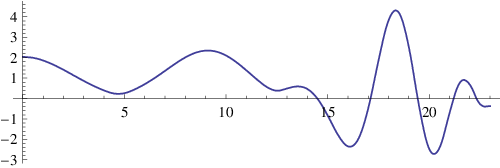
Refer to caption — Figure 3.1. The $Z$ -function of an $L$ -function satisfying functional equation (2.3) with $d=4$ and $\mu_{1}=-\mu_{2}=4.7209i$ and $\mu_{3}=-\mu_{4}=12.4687i$ . The first zeros are at $\pm\gamma_{1}=14.496$ . Data taken from [FKL].

The plot in Figure 3.1 shows local minima near 4.7 and 12.5. Those are due to the trivial zeros, which have imaginary parts $-\Im(\mu_{j})$ . Those trivial zeros suppress the appearance of nearby zeros on the critical line, a phenomenon first observed by Strombergsson [St]. Thus, such $L$ -functions can have a surprisingly large gap between their critical zeros.

For the reader who may wish to check our calculations, such as with the explicit formula, we provide the spectral parameters and initial Dirichlet coefficients to higher precision:

$\displaystyle\mu_{1}=\mathstrut$	$\displaystyle 4.72095103638565339773$	(3.1)
$\displaystyle\mu_{2}=\mathstrut$	$\displaystyle 12.4687522615131728082$	(3.2)
		(3.3)
$\displaystyle a_{2}=\mathstrut$	$\displaystyle\phantom{\mathstrut-\mathstrut}1.34260324197021624329$	(3.4)
$\displaystyle a_{3}=\mathstrut$	$\displaystyle-0.18745190876087089719$	(3.5)
$\displaystyle a_{4}=\mathstrut$	$\displaystyle\phantom{\mathstrut-\mathstrut}0.4644565335271682550$	(3.6)
$\displaystyle a_{5}=\mathstrut$	$\displaystyle-0.001627934631772515$	(3.7)
$\displaystyle a_{7}=\mathstrut$	$\displaystyle\phantom{\mathstrut-\mathstrut}0.22822958260580737$	(3.8)
$\displaystyle a_{9}=\mathstrut$	$\displaystyle-0.4634288260750947$	(3.9)
$\displaystyle a_{11}=\mathstrut$	$\displaystyle\phantom{\mathstrut-\mathstrut}0.695834471444353$	(3.10)
$\displaystyle a_{13}=\mathstrut$	$\displaystyle-0.8824356594477$	(3.11)

Note also that the zeros with imaginary part $0<\gamma<30$ are at the heights $\{$ 14.4960615091, 17.1144514545, 19.4393573576, 21.193378013, 22.396088469, 23.108950059, 24.34252975, 25.59506020, 27.12281351, 28.2791393, 29.5857431 $\}$ .

4. An upper bound on gaps between zeros

4.1. The explicit formula

We use Weil’s explicit formula with a particular test function to establish Theorem 2.1.

The form of the explicit formula that we will use is the following.

Lemma 4.1.

Suppose that $L(s)$ has a Dirichlet series expansion (2.1) which continues to an entire function such that

\Lambda(s)=Q^{s}\prod_{j=1}^{d}\Gamma_{\mathbb{R}}\left(s+\mu_{j}\right)L(s)=\varepsilon\overline{\Lambda(1-\overline{s})}

(4.1)

is entire and satisfies the mild growth condition $L(\sigma+it)\ll|t^{A}|$ , uniformly in $t$ for bounded $\sigma$ . Let $f(s)$ be holomorphic in a horizontal strip $-(1/2+\delta)<\Im(s)<1/2+\delta$ with $f(s)\ll\min(1,|s|^{-(1+\epsilon)})$ in this region, and suppose that $f(x)$ is real valued for real $x$ . Suppose also that the Fourier transform of $f$ defined by

\hat{f}(x)=\int_{-\infty}^{\infty}f(u)e^{-2\pi iux}dx

is such that

\sum_{n=1}^{\infty}\frac{c(n)}{n^{1/2}}\hat{f}\left(\frac{\log{n}}{2\pi}\right)+\frac{\overline{c(n)}}{n^{1/2}}\hat{f}\left(-\frac{\log n}{2\pi}\right)

converges absolutely, where $c(n)$ is defined by

\frac{L^{\prime}}{L}(s)=\sum_{n=1}^{\infty}\frac{c(n)}{n^{s}}.

(4.2)

Then

	$\displaystyle\sum_{\gamma}f(\gamma)=\mathstrut$	$\displaystyle\frac{\widehat{f}(0)}{\pi}\log{Q}+\frac{1}{2\pi}\sum_{j=1}^{d}\ell(\mu_{i},f)$		(4.3)
		$\displaystyle+\frac{1}{2\pi}\sum_{n=1}^{\infty}\frac{c(n)}{n^{1/2}}\hat{f}\left(\frac{\log{n}}{2\pi}\right)+\frac{\overline{c(n)}}{n^{1/2}}\hat{f}\left(-\frac{\log n}{2\pi}\right)$		(4.4)

where

\ell(\mu,f)=\Re\left\{\int_{\mathbb{R}}\frac{\Gamma^{\prime}}{\Gamma}\left(\frac{1}{2}\left(\frac{1}{2}+it\right)+\mu\right)f(t)dt\right\}-\hat{f}(0)\log\pi

(4.5)

and the sum $\sum_{\gamma}$ runs over all non-trivial zeroes of $L(s)$ .

Proof.

This can be found in Iwaniec and Kowalski [IK, Page 109], but note that they use a different normalization for the Fourier transform. ∎

Note that if we assume the Ramanujan-Petersson conjecture then $c(n)\ll n^{\epsilon}$ , but any mild growth estimate on the $c(n)$ is sufficient for our purposes.

The general strategy we will use is as follows: to show that $L(1/2+it)$ has a zero with $\alpha\leq t\leq\beta$ , we want to take $f$ to be a good approximation of $\chi_{(\alpha,\beta)}$ , the step function with value $1$ on $(\alpha,\beta)$ and $0$ elsewhere, and such that the support of $\hat{f}$ is contained in the interval $\left(-\frac{\log{2}}{2\pi},\frac{\log{2}}{2\pi}\right)$ . Then, the last sum on the RHS of the explicit formula disappears, and for the $L$ -functions that we are considering, (4.3) should look like

\sum_{\alpha<\gamma<\beta}f(\gamma)\approx\frac{\log Q}{\pi}\hat{f}(0)+\frac{1}{2\pi}\sum_{j=1}^{d}\ell(\mu_{j},f).

(4.6)

Since $f$ approximates $\chi_{(\alpha,\beta)}$ , we expect that

\ell(\mu_{j},f)\approx\Re\left\{\int_{\alpha}^{\beta}\left(\frac{\Gamma^{\prime}}{\Gamma}\left(\frac{1}{4}+\frac{it}{2}+\mu_{j}\right)\right)dt\right\}-(\beta-\alpha)\log\pi.

If $\beta-\alpha$ is large enough then this will be positive for any $\mu_{j}$ . We will then find that the right side of (4.6) is positive, which shows the existence of the zero that we are looking for.

While we cannot actually use the characteristic function of the interval $(\alpha,\beta)$ in the explicit formula, we do not quite need to. As long as $f(x)$ is positive for $\alpha<x<\beta$ and negative elsewhere, the same argument will work. The function which we use here is the Selberg minorant $S_{-}(z)$ for the interval $(\alpha,\beta)$ and with Fourier transform supported in $(-(\log 2)/2\pi,(\log 2)/2\pi)$ . We describe this function below. Note that with this approach there are fundamental limits to how small we can make $\beta-\alpha$ . According to the uncertainty principle, we should need to make the support of $\hat{f}$ large if we want to get a good function with $\beta-\alpha$ small.

4.2. Selberg’s amazing functions

As we have already described, we would like to use in the explicit formula a function $f(x)$ which is positive only in a prescribed interval and which has a compactly supported Fourier transform. Additionally, we have some reason to believe that a good candidate for our purposes should be close to $1$ inside this interval and close to $0$ outside of it. Selberg [Se, pages 213–225] gives a construction of such functions which are suitable for our purposes.

These functions are easiest to describe by first defining the Beurling function

B(z)=1+2\left(\frac{\sin\pi z}{\pi}\right)^{2}\left(\frac{1}{z}-\sum_{n=1}^{\infty}\frac{1}{(n+z)^{2}}\right).

This function is a good approximation for the function

\mathrm{sgn}(x)=\left\{\begin{array}[]{cl}1&\textrm{if }x>0\\ 0&\textrm{if }x=0\\ -1&\textrm{if }x<0\end{array}\right.

and it is a majorant for $\mathrm{sgn}(x)$ ; that is, $\mathrm{sgn}(x)\leq B(x)$ for all real $x$ . Beurling (unpublished) showed that this is the best possible such approximation in the sense that if $F(z)$ is any entire function satisfying $\mathrm{sgn}(x)\leq F(x)$ for all real $x$ and $F(z)\ll_{\epsilon}\exp((2\pi+\epsilon)|z|)$ , then

\int_{-\infty}^{\infty}\left(F(x)-\mathrm{sgn}(x)\right)\ dx\geq 1,

with equality achieved if and only if $F(x)=B(x)$ . (A proof can be found in [V].)

To approximate the characteristic function of an interval, we can use a simple linear combination of Beurling functions.

Definition 4.2.

The Selberg minorant $S_{-}(z)$ for the interval $[\alpha,\beta]$ and parameter $\delta>0$ is defined by

S_{-}(z)=-\frac{1}{2}\Big(B(\delta(\alpha-z))+B(\delta(z-\beta))\Big)

Selberg [Se, pages 213–225] proved that whenever $\delta(\beta-\alpha)$ is an integer, $S_{-}(z)$ is a best possible minorant for the characteristic function of the interval $[\alpha,\beta]$ , in the same sense that $B(z)$ is the best possible majorant for the $\mathrm{sgn}$ function, although $S_{-}(z)$ is not the unique best possible minorant. We do not make us of this extremal property anywhere, but it is the motivation behind our choice of using $S_{-}(z)$ in the explicit formula, and it may give hope that our results are not too far from optimal.

We summarize some important properties of $S_{-}(z)$ that we do need in the following lemma.

Lemma 4.3.

Let $S_{-}(z)$ be the Selberg minorant for the interval $[\alpha,\beta]$ with parameter $\delta$ . Then the following hold.

(1)

$S_{-}(x)\leq\chi_{(\alpha,\beta)}(x)$ for all real $x$ .
(2)

$\int_{-\infty}^{\infty}S_{-}(x)dx=\beta-\alpha-\frac{1}{\delta}$ .
(3)

$\hat{S}_{-}(x)=0$ for $x>\delta$ or $x<-\delta$ .
(4)

For any $\epsilon>0$ , $S_{-}(z)\ll_{\delta,\alpha,\beta,\epsilon}\min\left(1,\frac{1}{|z|^{2}}\right)$ for $\Im(z)\leq\epsilon$ .

Proof.

All of these facts can be found in Selberg’s work [Se, pages 213–225]. ∎

Remark.

For the function $f$ that we choose in the explicit formula, we will also need $f(x)>0$ in a prescribed range. If $\delta(\beta-\alpha)$ is too small, then this might not be the case for the function $S_{-}(x)$ . With the specific parameters we choose, this will hold for our application, however.

4.3. Proof of Theorem 2.1

Sketch of proof of Theorem 2.1.

Lemma 4.3 tells us that in the formula we may choose $f(s)=S_{-}(s)$ . We do so, with $\alpha=-2.5/\delta$ and $\beta=2.5/\delta$ , where $\delta=\frac{\log 2}{2\pi}$ . The explicit formula then reads

\sum_{\gamma}S_{-}(\gamma)=\frac{\log Q}{\pi}\hat{S}_{-}(0)+\frac{1}{2\pi}\sum_{j=1}^{d}\Re\left\{\int_{-\infty}^{\infty}\frac{\Gamma^{\prime}}{\Gamma}\left(\frac{1}{4}+\frac{it}{2}+\mu_{j}\right)S_{-}(t)dt\right\}-\frac{d}{2\pi}\hat{S}_{-}(0)\log\pi

(4.7)

Since $\hat{S}_{-}(0)=4/\delta$ is positive and $Q\geq 1$ , we may ignore the first term of this sum in establishing a lower bound. We then can check that

\Re\left\{\int_{-\infty}^{\infty}\frac{\Gamma^{\prime}}{\Gamma}\left(\frac{1}{4}+\frac{it}{2}+\mu\right)S_{-}(t)dt\right\}>\hat{S}_{-}(0)\log\pi

for all choices of $\mu$ . The right hand side of (4.7) is thus positive. As $S_{-}(\gamma)$ is only positive when $\alpha<\gamma<\beta$ , we conclude that $L(1/2+i\gamma)=0$ for some $\gamma$ in this range.

More details of this computation will appear in [B]. ∎

Remark.

Note that $\beta-\alpha\approx 45.3236$ . It should be possible to use the Selberg functions to make this difference a very little bit smaller without changing the proof, but not much. We have chosen $\alpha$ and $\beta$ as above because the Selberg function has a much nicer representation when $(\beta-\alpha)\delta$ is an integer, which simplifies computation.

5. Positivity and non-existence of $L$ -functions

Although Miller’s paper [M] concerns $L$ -functions of real archimedean type, the methods also apply to the $L$ -functions considered here. When that approach is used on degree 3 or degree 4 $L$ -functions with functional equation (2.3) and $\mu_{j}$ pure imaginary, the result is not quite conclusive. Miller’s implementation involves two calculations. One calculation shows that if all the $\mu_{j}$ are sufficient small (i.e., lying in a certain bounded region which can be made explicit) then such an $L$ -function cannot exist. The second calculation shows that if the $\mu_{j}$ lie outside another (possibly larger) region, then the $L$ -function must have a zero with imaginary part less than $14$ .

For $d=3$ or $4$ , those two calculations do not resolve whether or not there is an $L$ -function with a first zero higher than the Riemann zeta function, because there remains a very small region which could possibly correspond to an $L$ -function. And if such an $L$ -function exists, one would then need to calculate its first zero to check if it was higher than 14.13. For the case of $d=3$ , calculations of Bian [Bi, FKL] show that there are no $L$ -functions in the missing region. Details are given by Bober [B].

But for $d=4$ , calculations in [FKL] suggest that there is an $L$ -function in the missing region. This is somewhat surprising because that region is very small, as shown in Figure 5.1. Furthermore, as was shown in Figure 3.1, that $L$ -function has a larger gap between its zeros than does the Riemann zeta function. Note: the example from [FKL] was found prior to our implementation of Miller’s inequalities for $d=4$ . Specifically, that $L$ -function was found from a general search for degree-4 $L$ -functions, not merely from an attempt to find examples of $L$ -functions with a high lowest zero. Perhaps that makes it even more surprising that such an example exists.

References

[Bi] Ce Bian, Computing GL(3) automorphic forms, Bull. Lond. Math. Soc. 42 (2010), no. 5, 827–842.
[B] Jonathan Bober, Bounds for large gaps between zeros of $L$ -functions, preprint.
[FKL] David W. Farmer, Sally Koutsoliotas, and Stefan Lemurell, Maass forms on $GL(3)$ and $GL(4)$ , to appear in IMRN.
[IK] Henryk Iwaniec and Emmanuel Kowalski, Analytic number theory. American Mathematical Society Colloquium Publications, 53. American Mathematical Society, Providence, RI, 2004.
[M] Stephen D. Miller, The Highest-Lowest Zero and other Applications of Positivity, Duke Math. J. Volume 112, Number 1 (2002), 83-116.
[O] Andrew Odlyzko, Bounds for discriminants and related estimates for class numbers, regulators and zeroes of zeta functions: a survey of recent results, Séminaire de Théorie des Nombres, Bordeaux 2 (1990), 119–141.
[Se] Atle Selberg, Collected Papers. Volume II. Springer-Verlag, Berlin, 1991
[St] Andreas Strombergsson, On the zeros of $L$ -functions associated to Maass waveforms. Internat. Math. Res. Notices 1999, no. 15, 839–851
[T] E.C. Titchmarsh, The theory of the Riemann zeta-function, 2nd Edition, Oxford University Press, 1986.
[V] Jeffrey D. Vaaler, Some extremal functions in Fourier analysis. Bull. Amer. Math. Soc. (N. S.) Volume 12, Number 2 (1985), 183–216.
[Y] Hiroyuki Yoshida, On calculations of zeros of various $L$ -functions, J. Math. Kyoto University, vol 35(1995), 663-696.

The highest lowest zero of general L-functions

Abstract.

1. Introduction

2. LL-functions

Theorem 2.1.

Question 2.2.

Question 2.3.

3. A certain degree-4 LL-function

4. An upper bound on gaps between zeros

4.1. The explicit formula

Lemma 4.1.

Proof.

4.2. Selberg’s amazing functions

Definition 4.2.

Lemma 4.3.

Proof.

Remark.

4.3. Proof of Theorem 2.1

Sketch of proof of Theorem 2.1.

Remark.

5. Positivity and non-existence of LL-functions

References

2. $L$ -functions

3. A certain degree-4 $L$ -function

5. Positivity and non-existence of $L$ -functions