Probabilistic Catalogs for Crowded Stellar Fields

Brendon J. Brewer ^†^†thanks: bj.brewer@auckland.ac.nz Affiliation: Department of Statistics, The University of Auckland, Private Bag 92019, Auckland 1142, New Zealand Daniel Foreman-Mackey Affiliation: Center for Cosmology and Particle Physics, Department of Physics, New York University, Washington Place, New York, NY, 10003, USA David W. Hogg Affiliation: Center for Cosmology and Particle Physics, Department of Physics, New York University, Washington Place, New York, NY, 10003, USA

Abstract

We present and implement a probabilistic (Bayesian) method for producing catalogs from images of stellar fields. The method is capable of inferring the number of sources $N$ in the image and can also handle the challenges introduced by noise, overlapping sources, and an unknown point spread function (PSF). The luminosity function of the stars can also be inferred even when the precise luminosity of each star is uncertain, via the use of a hierarchical Bayesian model. The computational feasibility of the method is demonstrated on two simulated images with different numbers of stars. We find that our method successfully recovers the input parameter values along with principled uncertainties even when the field is crowded. We also compare our results with those obtained from the SExtractor software. While the two approaches largely agree about the fluxes of the bright stars, the Bayesian approach provides more accurate inferences about the faint stars and the number of stars, particularly in the crowded case.

Keywords:

catalogs — methods: data analysis — methods: statistical — stars: luminosity function, mass function

I Introduction

Traditional practice in astronomy is to take images of the sky, detect or enumerate sources visible in those images, and create catalogs. These catalogs are then used to perform fundamental astronomical measurements, for example reconstructing the three-dimensional structure of the Galaxy or the two-point correlation function of galaxies. Indeed, the process of catalog construction is so “baked in” to our ideas about what astronomy is, we sometimes forget that the catalog is not the fundamental data product of astronomy; catalogs are produced from imaging; their production involves many decisions and ideas that go beyond the information provided to the telescope by the incident intensity field. In addition, catalogs are not usually the final goal of any imaging project or survey. Typically, they are produced in order to facilitate the scientific study of populations of objects (e.g. the initial mass function of a population of stars), or to provide a sky-search capability to the community who might be interested in only a small subset of objects. Standard tools for generating catalogs from astronomical imaging include SExtractor [1], DAOPHOT [29], DOLPHOT [6], and SDSS Photo [22].

Telescopes don’t make catalogs [15], they measure the intensity field. Viewed through the lens of probabilistic inference, the goals of astronomy are to take the information in the telescope-generated records of the intensity field and use this information to obtain quantities of astronomical interest with as little loss as possible. Insertion of a catalog-generation step in the inference pipeline between the raw imaging and the final astrophysical analyses is potentially lossy. The hard decisions of catalog making destroy information, at least in principle. Probability theory suggests that it may be less lossy to pass forward not a catalog but a probabilisitic description of all the catalogs that could be consistent with the imaging—a posterior probability distribution in the (enormously large) space of possible catalogs. Essentially, the creation of a catalog is an attempt to answer the question, “Given the image we have obtained, what objects are present in the field and what are their properties?”. This article represents an attempt at implementing this ambitous goal in the specific situation where the only objects in the field are stars or other point sources.

Beyond these philosophical concerns, there are practical issues; standard methods for constructing catalogs can have difficulty in some challenging situations. For example, when multiple sources overlap partially or completely, it can be difficult to determine how many sources are present, and how much flux belongs to each source. In principle, the uncertainty about the existence and properties of the objects can be significant and should be propagated into any inferences about the stellar population. A Bayesian approach that obtains the posterior distribution over catalog space (rather than a single catalog estimate) has the potential to overcome these problems by deblending objects when it is possible, and clearly indicating the uncertainty remaining when it is not possible.

In practice, Bayesian Inferences are often implemented using Markov Chain Monte Carlo (MCMC) methods [23] to sample from the posterior distribution. Sampling a posterior probability distribution for catalogs is a challenging numerical task for a number of reasons. Firstly, the number $N$ of objects in the image (and that should therefore be listed in the catalog) is itself unknown. Secondly, if $N$ is large, then the parameter space of positions and properties (flux, size, etc) of the objects is also large. This can cause Markov Chain Monte Carlo (MCMC) algorithms difficulties – they may take a long time to converge to the target posterior distribution over the space of catalogs. Thirdly, this problem is subject to the so-called label-switching problem that is commonly encountered in mixture modeling [17, e.g.]. Given any proposed catalog, another catalog that is equally plausible is the catalog obtained by shuffling the entries of the first catalog. This leads to a posterior distribution with $N!$ identical peaks in parameter space. This can lead to difficulties with certain (otherwise very effective) MCMC algorithms such as the affine-invariant stretch move [10, 9].

Bayesian object detection (as this problem is sometimes called) has been implemented both inside and outside of astronomy [12, 13, 7, e.g.]. However, the Feroz et al. [7] approach makes the assumption of a known number of objects $N$ . This assumption is required for the MultiNest sampler [8] to be applicable. Using the results from the known $N$ run, it is possible (under certain circumstances) to reconstruct what the results would have been if an unknown- $N$ model had been used. However, this will not work well in situations where there is significant confusion (i.e. two or more sources overlap). What is really required is a variable dimension model, where $N\in\{0,1,2,...\}$ is an unknown quantity to be inferred from the data [13, e.g.]. The computational implementation of these models will require tools such as reversible jump Markov Chain Monte Carlo [11]. Other statistical methods have also been used to model crowded fields [16, e.g. maximum likelihood,]. However, maximum likelihood is not completely appropriate in flexible models because it may lead to overfitting. In this situation overfitting would result in more stars being added to the model to explain small positive fluctuations in the image which are actually due to noise. Various other techniques have also been proposed in the literature [25, 24, 30, e.g.].

In this paper, we develop a Bayesian object detection model with the following features: i) the number $N$ of objects in the image is an unknown parameter to be inferred from the data, ii) the objects that we expect to find are point sources such as stars, and iii) the point-spread function is unknown (but a parametric model is used) and must be inferred from the data (but a single bright star may not be available to help with estimating it). The paper is structured as follows. In Section II we give a brief overview of Bayesian inference. In Section III we discuss the model assumptions we make in our method. In Section IV we briefly discuss our MCMC implementation. Section V describes the tests we carried out on simulated data, and a comparison with SExtractor results is presented in Section VI. We conclude in Section VII.

II Bayesian Inference

To quantitatively model uncertainties and transform noise in observed data into uncertainties in parameters of interest, Bayesian Inference is the appropriate framework [5, 18, 4, 23]. Suppose there exist unknown parameters (denoted collectively by $\theta$ ) and we expect to obtain some data $x$ . Our prior state of knowledge about the parameters is modelled by a prior probability distribution:

p(\theta).

(1)

Note that this is a very concise notation [14] and should be read as, “The probability distribution for $\theta$ ”. We also model how the parameters give rise to the data, via a generative model. This is also known as a sampling distribution:

p(x|\theta).

(2)

Despite the singular, the sampling distribution is actually a family of probability distributions over the space of possible data sets, one probability distribution for each possible value of $\theta$ . Note that the choice of the sampling distribution is also an assumption about prior knowledge: It models prior information about the fact that the data $x$ is connected to the parameters $\theta$ in some way [4]. Without this prior knowledge, learning is impossible: there has to be some relationship between the parameters and the data, otherwise it would be impossible to learn about parameters by obtaining data.

When specific data $x^{*}$ are taken into account, our state of knowledge about $\theta$ gets updated from the prior distribution to the posterior distribution via Bayes’ rule:

	$\displaystyle p(\theta\|x=x^{*})$	$\displaystyle\propto$	$\displaystyle p(\theta)p(x\|\theta)\|_{x=x^{*}}$		(3)
		$\displaystyle=$	$\displaystyle p(\theta)\mathcal{L}(\theta;x)$		(4)

The term $p(x|\theta)|_{x=x^{*}}=\mathcal{L}(\theta;x)$ is the likelihood function, which is the probability of obtaining the actual data set $x^{*}$ as a function of the parameters. In the case that the sampling distribution is a probability density function, the likelihood is the probability density function evaluated at the observed data. This usually causes no problems, although one should be aware of the Borel-Kolmogorov paradox [18]. As suggested by the above notation, the likelihood function is obtained from the sampling distribution with the actual data substituted in and is therefore a function of the parameters only.

To proceed with the model for inferring catalogs from image data, we must specify a definite hypothesis space and choices for the prior distribution and the sampling distribution. These choices are presented and discussed in Section III.

III The Specific Model for Stellar Fields

III.1 The Hypothesis Space

The hypothesis space is the set of possible catalogs, or the set of possible answers to the question, “What objects are present in the field and what are their properties?” We shall assume that there are an unknown number of stars $N$ in the field. Each star has an unknown position $(x,y)$ in the plane of the sky, and an unknown flux $f$ . We also describe the distribution of fluxes (commonly known as the luminosity function) of the stars by some parameters denoted collectively by $\beta$ . In summary, the unknown parameters are:

\displaystyle\theta=\left\{N,\beta,\left\{x_{i},y_{i}\right\}_{i=1}^{N},\left\{f_{i}\right\}_{i=1}^{N}\right\}.

(5)

We note that models similar to this have been implemented for general image modeling and deconvolution [27, e.g.], however in this case it is more justified as we are actually searching for point fluxes.

III.2 The Prior

The prior probability distribution for the unknown parameters can be factorized using the product rule of probability theory. With a variety of independence assumptions, the prior can be factorized as:

\displaystyle p(\theta)=p(\beta)p(N|\beta)\prod_{i=1}^{N}p(x_{i},y_{i})p(f_{i}|\beta)

(6)

Here, we have assumed that the luminosity function does not depend on position. Finally, the fluxes of the stars come independently from a common distribution. If we knew the luminosity function of the stars, then the location and flux of a particular star would not tell us anything about the location and flux of another star. Really, this is just a way of implementing exchangeability of the stars, and is often called a hierarchical model.

For simplicity, we assume a uniform prior probability distribution for the position of each star. The use of independent priors for the positions creates a strong preference for catalogs where the stars are uniformly scattered across the image. Thus, this model is appropriate for small images where the density of stars is approximately uniform across the image. In other scenarios, such as images of stellar clusters, it is possible to parameterize the spatial distribution of the stars in a similar way to how we have parameterized the luminosity function, i.e. as a hierarchical model.

III.3 The Sampling Distribution

The sampling distribution is a probabilistic model for the process that generates the data; it describes the probability distribution we would use to predict the data if we happened to know the true catalog. In our case, the data will be an $m\times n$ array of pixel intensities $I$ :

\displaystyle\{I_{ij}\}

(7)

where the central position of each pixel is:

\displaystyle\{X_{ij},Y_{ij}\}.

(8)

The image is assumed to be a noisy version of the true underlying intensity field. Thus, we need a prescription for simulating an image $\{I_{ij}\}$ from a catalog $\theta$ :

\displaystyle\theta=\left\{N,\beta,\left\{x_{i},y_{i}\right\}_{i=1}^{N},\left\{f_{i}\right\}_{i=1}^{N}\right\}.

(9)

If we knew the true catalog, we could compute the “mock image” we would expect to see in the absence of noise. This mock image (defined at every point on the sky) is given by:

\displaystyle\mathcal{M}(x,y)

\displaystyle=

\displaystyle\sum_{i=1}^{N}f_{i}\mathcal{P}(x-x_{i},y-y_{i})

(10)

where $\mathcal{P}$ is the pixel-convolved point spread function (PSF). The use of a pixel-convolved PSF is computationally advantageous because the PSF need only be evaluated at the center of each pixel, rather than integrated over each pixel.

Throughout this paper we will assume the pixel-convolved PSF is a weighted mixture of two concentric circular Gaussians (a similar mixture model that uses a Gaussian core and flexible wings is also used by DAOPHOT, Stetson [29]) with widths $s_{1}$ and $s_{2}$ :

\displaystyle\mathcal{P}(x,y)=\frac{w}{2\pi s_{1}^{2}}\exp\left[-\frac{1}{2s_{1}^{2}}\left(x^{2}+y^{2}\right)\right]+\frac{1-w}{2\pi s_{2}^{2}}\exp\left[-\frac{1}{2s_{2}^{2}}\left(x^{2}+y^{2}\right)\right].

(11)

The pixellated observed image is assumed to be generated from the mock image (evaluated at the center of each pixel) plus noise:

\displaystyle I_{ij}

\displaystyle=

\displaystyle\mathcal{M}(X_{ij},Y_{ij})+\epsilon_{ij}

(12)

where the errors $\{\epsilon_{ij}\}$ are independent and normally distributed. The variance of the normal distribution for each pixel is determined by the brightness of the sky and the brightness of the mock image in that pixel. This can be modelled by assuming the following distribution:

\displaystyle\epsilon_{ij}\sim\mathcal{N}(0,\sigma_{0}^{2}+\eta\mathcal{M}(X_{ij},Y_{ij})).

(13)

where $\sigma_{0}$ is a constant noise level and $\eta$ is an unknown = coefficient that allows for the possibility that the noise level is higher in brighter regions of the image. This dependence of the noise variances on the model intensity arises as a result of the Poissonian nature of photon counts, but allows for the fact that a “sky” background may have already been subtracted from the image in the reduction process. This parameterisation has been used by Brewer et al. [3] and is an alternative to the common practice of producing a “variance map” from the image data that is then assumed to be known.

III.4 The Prior Distribution

The prior distribution for the number of stars $N$ is assigned to be uniform between 0 and some maximum number $N_{\rm max}$ . The extent of the image is assumed to be from $x=x_{\rm min}$ to $x=x_{\rm max}=x_{\rm min}+x_{\rm range}$ and from $y=y_{\rm min}$ to $y=y_{\rm max}=y_{\rm min}+y_{\rm range}$ in arbitrary units, and the positions of the stars are assigned independent uniform priors:

	$\displaystyle x_{i}$	$\displaystyle\sim$	$\displaystyle\textnormal{Uniform}(x_{\rm min}-0.1x_{\rm range},x_{\rm max}+0.1x_{\rm range})$		(14)
	$\displaystyle y_{i}$	$\displaystyle\sim$	$\displaystyle\textnormal{Uniform}(y_{\rm min}-0.1y_{\rm range},y_{\rm max}+0.1y_{\rm range})$		(15)

The stars are allowed to be slightly outside of the observed image because the PSF can scatter light from these stars into the image.

For the purposes of this paper, we model the luminosity function as a broken power-law distribution, which has four free parameters:

\displaystyle\beta=\{h_{1},h_{2},\alpha_{1},\alpha_{2}\}.

(16)

where $h_{1}$ is a lower flux limit, $h_{2}$ is a break-point, $\alpha_{1}$ is the slope of the distribution between $h_{1}$ and $h_{2}$ , and $\alpha_{2}$ is the slope of the distribution above $h_{2}$ . For mathematical details on the broken power-law model, see Appendix A. While the broken power-law is likely to be unrealistic in many cases, it is a reasonably flexible distribution and this is sufficient for demonstrating the properties of our method.

The prior distribution on $h_{1}$ , $h_{2}$ , $\alpha_{1}$ , and $\alpha_{2}$ is assigned to be:

$\displaystyle\ln h_{1}$	$\displaystyle\sim$	$\displaystyle\textnormal{Uniform}(\ln(10^{-3}),\ln(10^{3}))$	(17)
$\displaystyle\ln h_{2}$	$\displaystyle\sim$	$\displaystyle\textnormal{Uniform}(\ln(h_{1}),\ln(h_{1})+2.3)$	(18)
$\displaystyle\alpha_{1}$	$\displaystyle\sim$	$\displaystyle\textnormal{Uniform}(1,5)$	(19)
$\displaystyle\alpha_{2}$	$\displaystyle\sim$	$\displaystyle\textnormal{Uniform}(1,5).$	(20)

These priors express vague prior knowledge about $\alpha_{1}$ and $\alpha_{2}$ in addition to vague prior knowledge about $h_{1}$ and $h_{2}$ apart from the fact that the flux units are not extreme and that $h_{2}$ should be no more than an order of magnitude greater than $h_{1}$ .

This simply-parameterized model for the luminosity function can be criticized on the basis that information from bright stars can be used to infer the parameters of the luminosity function which then still apply at lower flux levels. In principle, this can be resolved by using a more flexible distribution [19, e.g.] where each star’s measured brightness affects the inference of the luminosity function locally but not globally.

The priors for the PSF parameters and the noise parameters were assigned to be:

$\displaystyle\ln s_{1}$	$\displaystyle\sim$	$\displaystyle\textnormal{Uniform}(\ln(0.3L),\ln(30L))$	(21)
$\displaystyle\ln s_{2}$	$\displaystyle\sim$	$\displaystyle\textnormal{Uniform}(\ln(s_{1}),\ln(s_{1})+2.3)$	(22)
$\displaystyle w$	$\displaystyle\sim$	$\displaystyle\textnormal{Uniform}(0,1)$	(23)
$\displaystyle\ln\sigma_{0}$	$\displaystyle\sim$	$\displaystyle\textnormal{Uniform}(\ln(10^{-3}),\ln(10^{3}))$	(24)
$\displaystyle\ln\eta$	$\displaystyle\sim$	$\displaystyle\textnormal{Uniform}(\ln(10^{-3}),\ln(10^{3}))$	(25)

where $L=x_{\rm range}/n$ is the width of a pixel. These priors describe vague prior knowledge about the overall scale of the PSF except that the wider component is less than 10 times as wide as the narrow component, as well as the knowledge that the noise variance is not extreme relative to the fluxes of the stars.

IV MCMC Implementation

The MCMC sampling was implemented using the Diffusive Nested Sampling [2] method (hereafter DNS). DNS is a variant of the Nested Sampling [28] algorithm that uses Metropolis-Hastings updates, and is very generally applicable. The main difference between DNS and the standard Metropolis-Hastings algorithm is that the target distribution is modified. Rather than simply exploring the posterior distribution over catalog space, DNS constructs an alternative target distribution which is a mixture of the prior distribution with more constrained versions of the prior distribution. The modified target distribution assists the sampling in several ways. Firstly, the target distribution shrinks at a constant rate with time during the initial phase of the exploration. This is similar to the popular “simulated annealing” method [20, 26] but with an optimal annealing schedule. Secondly, communication with the prior is maintained: once a catalog is found that fits the data, the catalog can “disintegrate” back to the prior distribution and re-fit, allowing different peaks in the parameter space to be explored (if they exist). This all happens naturally within the context of a valid MCMC sampler. The MCMC may also be run using the standard Metropolis algorithm targeting the posterior distribution.

V Simulated Data

In order to test our approach, we applied the method to two illustrative simulated images generated from the above model (Figure 1). The purpose of this experiment was to test the computational feasibility of the model, as well as to compare the inferences from the model with those from more standard techniques.

The true parameter values for the two simulated data sets are listed in Table 1. The broken power-law parameter values were chosen so that roughly half of the stars’ fluxes were below and above the break-point respectively. Figure 7 in Appendix A also shows the true flux distribution used for the simulated images. Each of the images is $100\times 100$ pixels in extent and covers a range from $-1$ to $1$ in arbitrary units for both the $x$ and $y$ axes. The first image contains 100 stars (including stars just outside of the image; there are 63 stars whose central positions lie within the image) and the second image contains $\sim$ 1000 stars (699 of which are positioned within the image).

Parameter	Value (Test Case 1)	Value (Test Case 2)
$N$	100	1000
$h_{1}$	0.3	0.3
$h_{2}$	0.6	0.6
$\alpha_{1}$	1.1	1.1
$\alpha_{2}$	2	2
$\sigma_{0}$	10	10
$\eta$	10	10
$s_{1}$	0.02	0.02
$s_{2}$	0.1	0.1
$w$	0.5	0.5

Table 1: True parameter values used to generate the simulated data.

N

is the number of stars,

h_{1}

and

h_{2}

are the lower limit and break point of the flux distribution respectively, and

\alpha_{1}

and

\alpha_{2}

are the slopes of the flux distribution.

\sigma_{0}

and

\eta

describe the noise properties, and

s_{1}

s_{2}

, and

w

are the PSF parameters. The only difference between the two images is that Test Case 2 contains more stars than Test Case 1.

Refer to caption — Figure 1: The two simulated images used to test our methodology. Left: An image containing $\sim$ 100 stars. Right: An image containing $\sim$ 1000 stars.

V.1 Test Case 1

Test Case 1 was run with the DNS algorithm and usable results were obtained within about an hour on a modern desktop PC. The inferences on the parameters $N$ , $h_{1}$ , $h_{2}$ , $\alpha_{1}$ , and $\alpha_{2}$ are shown in Figure 2. The number of stars is correctly inferred, and the posterior distributions for the other parameters comfortably contain the true input values. As $N$ is a parameter of our model, there is no need for Bayesian “Model Comparison” calculations to be done between different values of $N$ . The DNS method does compute the “evidence” value that is required for model comparison, but this is useful only to test completely separate models, it is not needed to infer the value of $N$ .

Note that the uncertainty in $h_{2}$ , $\alpha_{1}$ , and $\alpha_{2}$ is quite large. This is because the broken power-law model (Figure 7) does not change drastically in shape as the parameters are varied. Therefore, a large number of stars would be required to tightly constrain these parameters.

The PSF parameters $\{s_{1},s_{2},w\}$ and the noise parameters $\{\sigma_{0},\eta\}$ were also inferred accurately with small uncertainties.

V.2 Test Case 2

Test Case 2 is more challenging than Test Case 1 because the image contains more stars. This increases the size of the computational task in two ways: firstly, there will be more unknown parameters to infer, so any MCMC algorithm will require more iterations in order to converge to the posterior distribution. Secondly, the time taken to compute the predicted image from a proposed catalog (in order to evaluate the likelihood) is longer because of the larger number of stars. Hence, each MCMC step also takes more time. Using DNS, some samples from the posterior distribution can be obtained in about a day on a modern multi-core PC.

Each catalog in the posterior sample represents a scenario for the true underlying image that we would observe if we had a hypothetical noise-free, infinite resolution telescope. Figure 4 shows nine possible catalogs sampled from the posterior distribution. Features that are common to these nine samples are plausible, and features that differ are uncertain.

From these samples, we can construct the posterior expected true scene and other summaries. Summary images are shown in Figure 5. The residuals provide a check on the validity of the model assumptions, and the posterior expected true scene provides a useful visual guide to the uncertainties present in the catalogs. In this example, the residuals show only noise because the simulated images were actually generated from the model.

The inferences on the number of stars $N$ and the luminosity function parameters are shown in Figure 3. The uncertainty about the luminosity function parameters is still considerable despite the larger number of stars, as the fluxes of the fainter stars are not well constrained by the data. The true values are still well within the range of plausible values in the posterior distribution. As with Test Case 1, the PSF parameters $\{s_{1},s_{2},w\}$ and the noise parameters $\{\sigma_{0},\eta\}$ were also inferred accurately with small uncertainties.

VI Comparison to SExtractor

In the previous section we established that the inference of the catalogs from the data is computationally feasible and that the number of stars and the luminosity function can be inferred from the image data, albeit with moderate uncertainties. We now compare this approach to an alternative analysis that makes use of the standard tool SExtractor [1]. To achieve this, we executed SExtractor on the two test images, for various values of the detection threshold parameters DETECT_THRESH and ANALYSIS_THRESH ranging from 0.5 to 6.5. This results in a set of catalogs for each image, with more conservative thresholds resulting in less stars detected as compared to more aggressive thresholds. To compute flux estimates that are directly comparable to the fluxes in our input catalogs, we configured SExtractor to compute object fluxes within fixed circular apertures that were known to contain 70% of the mass of the PSF. The SExtractor flux estimates were then scaled up to account for this finite aperture.

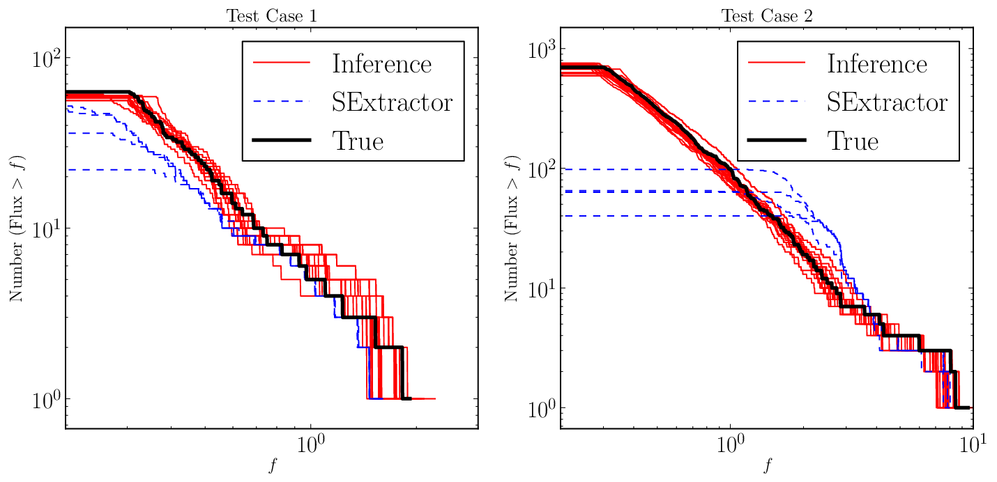
In Figure 6, we present the cumulative luminosity function (CLF) of the stars in the two fields, defined as the number of stars above a given flux. The true CLF is plotted along with several posterior samples from the Bayesian method and catalogs produced by SExtractor for various values of the detection and analysis thresholds. We note that the true CLF is typical of the posterior samples, as expected. For both test cases, the SExtractor catalog is also consistent with the posterior distribution at the bright end. However, the inferences from SExtractor and the Bayesian method differ at the faint end, with the former significantly underestimating the number of faint stars.

This result may be attributable to the fact that the Bayesian method knows about the existence and form of the luminosity function, even though it does not know the values of the parameters. To test this, we ran the inference on the data using an incorrect exponential distribution for the luminosity function. The resulting CLF from this run did undershoot the true CLF at the faint end. However, the Bayesian evidence for the exponential model was significantly lower (by a factor of approximately $10^{7}$ ) than for the (correct) broken power-law model.

In practice, we note that the wings of the PSF might become degenerate with an nonzero flat background level in the data. To test whether this was influencing the inferences (particularly about the faint end of the CLF) we also ran a model that included an unknown constant background. This had only a minor effect on the resulting inferences.

VII Discussion and Conclusions

In this paper we have developed and demonstrated a Bayesian approach to making catalogs from astronomical images in the case where the image contains only stars (or other point sources). The key idea is that instead of computing a single catalog, the method creates a posterior probability distribution on the space of possible catalogs that represents our state of knowledge about the presence and properties of objects in the image. When this is done, the uncertainties in the imaging are accurately propagated through to scientific conclusions, for example about the luminosity function of the stars. This approach was contrasted with the results from the standard SExtractor software. For the bright sources the results were essentially consistent, however the Bayesian approach was more successful at modelling the distribution of faint stars. Of course, the Bayesian method is much more computationally intensive, which is a significant issue in practice. However, the great value of upcoming imaging data sets and the irreproducibility of astronomical imaging data in areas of time-domain astrophysics (for example in observations of rare events) make it important to extract as much information as possible from every patch of imaging. Our view is that the additional CPU time and the non-triviality of the outputs from our method will be worth the effort in the next generation of astronomical experiments. To build a more complete picture of when our approach is necessary in practice, it will need to be tested against a wider variety of alternative methods such as DAOPHOT [29] and DOLPHOT [6].

We note that there are many limitations to the model presented in this paper, some of which will be important to relax when it is applied to real data. In principle, our model should be a model of the physical state of the universe, and not a simple model where the only stellar properties are a 2-D position and a flux. Another limitation is that we have not considered multi-epoch or multi-band imaging. In the former case, PSF variations and stellar motions may be relevant [21], and in the latter, a model for the spectral energy distributions of the stars will need to be considered: essentially, the luminosity function will need to be a probability distribution over more than one dimension.

In practice, it may also be necessary to improve the model for the prior distribution of stellar positions and fluxes. One area where this is clearly needed is the application of this approach to images of stellar clusters. The model would need to be revised to take into account the fact that we expect the stars’ positions to be clustered together, whereas the current model implies a large prior probability for the stars being scattered evenly across the image. In this and other applications, the luminosity function would also require multiple components, for example consisting of stars that are associated with a cluster or a stream and those that are not.

Throughout this paper, we have also assumed that the pixel-convolved PSF can be adequately modeled using simple components and that there are no PSF variations across the field. Relaxing these assumption provides a significant challenge for the future.

VIII Acknowledgements

It is a pleasure to thank Anna Nierenberg (UCSB), Jonathan Goodman (NYU), Fengji Hou (NYU), Dustin Lang (CMU), Andrew Dolphin (Raytheon), Julianne Dalcanton (Washington), Geraint Lewis (Sydney), and Phil Marshall (Oxford) for their comments and discussions. The referee is thanked for their thoughtful comments which helped us to improve the paper. BJB would like to thank Tommaso Treu (UCSB) for his support, and Wayne Stewart and Arden Miller (Auckland) for their encouragement and advice. DFM and DWH were partially supported by the US National Science Foundation (grant IIS-1124794) and the US National Aeronautics and Space Administration (grant NNX12AI50G).

Appendix A Broken Power-Law Distribution

The broken power-law distribution is based on a straightforward extension to a simple power-law distribution (also known as a Pareto distribution, particularly in the statistics literature). The power-law distribution for a variable $x$ (given a lower cutoff $x=h$ and a slope $\alpha$ ) is defined by:

\displaystyle p(x)

\displaystyle\propto

\displaystyle\left\{\begin{array}[]{lcl}0,&&x<h\\ x^{-\alpha-1}&&x\geq h.\end{array}\right.

In contrast, the broken power-law distribution for a variable $x$ is defined by a lower cutoff $x=h_{1}$ , two slopes $\{\alpha_{1},\alpha_{2}\}$ and a break point $x=h_{2}$ :

\displaystyle p(x)

\displaystyle\propto

\displaystyle\left\{\begin{array}[]{lcrl}0,&&x<h_{1}&\\ x^{-\alpha_{1}-1}&&h_{1}\leq x\leq h_{2}&\\ x^{-\alpha_{2}-1}&&x>h_{2}.\end{array}\right.

The free parameters of the broken power-law are:

\displaystyle\beta=\{h_{1},h_{2},\alpha_{1},\alpha_{2}\}.

(A8)

With normalising terms included, the proportionality becomes an equality:

\displaystyle p(x)

\displaystyle=

\displaystyle\left\{\begin{array}[]{lcr}0,&&x<h_{1}\\ Z_{1}^{-1}x^{-\alpha_{1}-1},&&h_{1}\leq x\leq h_{2}\\ Z_{2}^{-1}x^{-\alpha_{2}-1},&&x>h_{2}.\end{array}\right.

Two conditions will be used to determine the normalizers $Z_{1}$ and $Z_{2}$ . Firstly, the probability density function (PDF) should be continuous at $x=h_{2}$ :

	$\displaystyle Z_{1}^{-1}h_{2}^{-\alpha_{1}-1}$	$\displaystyle=$	$\displaystyle Z_{2}^{-1}h_{2}^{-\alpha_{2}-1}$		(A13)
	$\displaystyle\implies Z_{2}$	$\displaystyle=$	$\displaystyle Z_{1}h_{2}^{\alpha_{1}-\alpha_{2}}$		(A14)

The second condition is that the total probability must be 1:

$\displaystyle\int_{h_{1}}^{h_{2}}Z_{1}^{-1}x^{-\alpha_{1}-1}\,dx+\int_{h_{2}}^{\infty}Z_{2}^{-1}x^{-\alpha_{2}-1}\,dx$	$\displaystyle=$	$\displaystyle 1$	(A15)
$\displaystyle Z_{1}^{-1}\alpha_{1}^{-1}\left[h_{1}^{-\alpha_{1}}-h_{2}^{-\alpha_{1}}\right]+Z_{2}^{-1}\alpha_{2}^{-1}h_{2}^{-\alpha_{2}}$	$\displaystyle=$	$\displaystyle 1$	(A16)
$\displaystyle Z_{1}^{-1}\alpha_{1}^{-1}\left[h_{1}^{-\alpha_{1}}-h_{2}^{-\alpha_{1}}\right]+Z_{1}^{-1}h_{2}^{\alpha_{2}-\alpha_{1}}\alpha_{2}^{-1}h_{2}^{-\alpha_{2}}$	$\displaystyle=$	$\displaystyle 1$	(A17)

\displaystyle\implies Z_{1}

\displaystyle=

\displaystyle\alpha_{1}^{-1}\left[h_{1}^{-\alpha_{1}}-h_{2}^{-\alpha_{1}}\right]+h_{2}^{-\alpha_{1}}\alpha_{2}^{-1}.

(A18)

The cumulative distribution (CDF) is a useful property of a probability distribution and is given by the antiderivative of the PDF:

\displaystyle P(X\leq x)=F(x)

\displaystyle=

\displaystyle\left\{\begin{array}[]{lcr}0,&&x<h_{1}\\ (Z_{1}\alpha_{1})^{-1}\left(h_{1}^{-\alpha_{1}}-x^{-\alpha_{1}}\right),&&h_{1}\leq x\leq h_{2}\\ 1-(Z_{2}\alpha_{2})^{-1}x^{-\alpha_{2}},&&x>h_{2}.\end{array}\right.

The inverse of the CDF is also useful and is given by:

\displaystyle F^{-1}(u)

\displaystyle=

\displaystyle\left\{\begin{array}[]{lcr}\left[h_{1}^{-\alpha_{1}}-uZ_{1}\alpha_{1}\right]^{-1/\alpha_{1}},&&0<u<1-(Z_{2}\alpha_{2})^{-1}h_{2}^{-\alpha_{2}}\\ \left[Z_{2}\alpha_{2}(1-u)\right]^{-1/\alpha_{2}},&&1-(Z_{2}\alpha_{2})^{-1}h_{2}^{-\alpha_{2}}<u<1.\end{array}\right.

An example of a broken power-law distribution is shown in Figure 7.

Appendix B Proposal Distributions

To implement Metropolis-Hastings moves for the space of possible catalogs, proposal distributions are required. See Table 2 for a list of proposal distributions used in this study.

Parameter	Proposal	Notes
$N$	$N\to N+\delta_{N}$	Generate $\delta_{N}$ new stars from $p(x,y,f\|\beta)$ .
$N$	$N\to N-\delta_{N}$	Remove $\delta_{N}$ stars, chosen at random
$\beta$	$\beta\to\beta+\delta_{\beta}$	Transform stars’ fluxes correspondingly
$\beta$	$\beta\to\beta+\delta_{\beta}$	Fix stars’ fluxes, put extra term in acceptance probability
$(x_{i},y_{i})$	$(x_{i},y_{i})\to(x_{i},y_{i})+(\delta_{x},\delta_{y})$	Can move $>1$ star in a single step
$f$	$f\to f+\delta_{f}$	Can move $>1$ stars’ fluxes in a single step

Table 2: All

\delta

parameters are drawn from multi-scale distibutions such that the largest steps are of order the prior width, and the smallest steps are of order

10^{-6}

times the prior width.

References

[1] Bertin, E., Arnouts, S. 1996. SExtractor: Software for source extraction. Astronomy and Astrophysics Supplement Series 117, 393-404.
[2] Brewer B. J., Pártay L. B., Csányi G., 2011, Statistics and Computing, 21, 4, 649-656. arXiv:0912.2380
[3] Brewer, B. J., Lewis, G. F., Belokurov, V., Irwin, M. J., Bridges, T. J., Evans, N. W. 2011. Modelling of the complex CASSOWARY/SLUGS gravitational lenses. Monthly Notices of the Royal Astronomical Society 412, 2521-2529
[4] Caticha, A. 2009. Quantifying Rational Belief. American Institute of Physics Conference Series 1193, 60-68.
[5] Cox, R. T., 1946, Probability, Frequency, and Reasonable Expectation. 1946. American Journal of Physics 14 14, 1-13.
[6] Dolphin, A. E. 2000, PASP, 112, 1383
[7] Feroz, F., Balan, S. T., Hobson, M. P. 2011. Detecting extrasolar planets from stellar radial velocities using Bayesian evidence. Monthly Notices of the Royal Astronomical Society 415, 3462-3472.
[8] Feroz F., Hobson M. P., Bridges M., 2009, MNRAS, 398, 1601
[9] Foreman-Mackey, D., Hogg, D. W., Lang, D., & Goodman, J. 2012, emcee: The MCMC Hammer, arXiv:1202.3665
[10] Goodman, J., Weare, J., 2010, Ensemble Samplers with Affine Invariance, Comm. App. Math. Comp. Sci., 5, 6.
[11] Green, P. J., 1995, Reversible Jump Markov Chain Monte Carlo Computation and Bayesian Model Determination, Biometrika 82 (4): 711–732.
[12] Harkness, M. A. and Green, P. J., 2000, Parallel chains, delayed rejection and reversible jump MCMC for object recognition, British Machine Vision Conference Proceedings.
[13] Hobson, M. P., & McLachlan, C. 2003, MNRAS, 338, 765
[14] Hogg, D. W. 2012. Data analysis recipes: Probability calculus for inference. ArXiv e-prints arXiv:1205.4446.
[15] Hogg, D. W., Lang, D. 2011. Telescopes don’t make catalogues!. EAS Publications Series 45, 351-358.
[16] Irwin, M. J. 1985, MNRAS, 214, 575
[17] Jasra, A., Holmes, C. C, and Stephens, D. A., Markov Chain Monte Carlo Methods and the Label Switching Problem in Bayesian Mixture Modeling, Statistical Science Vol. 20, No. 1, pp. 50-67
[18] Jaynes, E. T., 2003, Probability Theory: The Logic of Science, ISBN 0521592712, Cambridge University Press, June 2003.
[19] Kelly, B. C., Fan, X., & Vestergaard, M. 2008, ApJ, 682, 874
[20] Kirkpatrick, S., Gelatt, C. D., Vecchi, M. P., 1983, Optimization by Simulated Annealing, Science 220 (4598): 671–680.
[21] Lang, D., Hogg, D. W., Jester, S., & Rix, H.-W. 2009, AJ, 137, 4400
[22] Lupton, R., Gunn, J. E., Ivezic, Z., Knapp, G. R., Kent, S. M., & Yasuda, N., 2001, ASPC, 238, 269
[23] Mackay, D. J. C., 2003, Information Theory, Inference and Learning Algorithms, Cambridge University Press, UK.
[24] Magain, P., Courbin, F., Gillon, M., et al. 2007, A&A, 461, 373
[25] Metchev, S. A., & Grindlay, J. E. 2002, MNRAS, 335, 73
[26] Neal, R. M., 2001, Annealed importance sampling, Statistics and Computing, vol. 11, pp. 125-139.
[27] Skilling J., 1998, Massive Inference and Maximum Entropy, in Maximum Entropy and Bayesian Methods, Kluwer Academic Publishers, Dordrecht/Boston/London p.14
[28] Skilling, J., 2006, Nested Sampling for General Bayesian Computation, Bayesian Analysis 4, pp. 833-860.
[29] Stetson, P. B. 1987, PASP, 99, 191
[30] Zhang, Z. W., Kim, D. W., Wang, J. H., et al. 2009, PASP, 121, 1429