Circuit complexity and Problem structure in Hamming space

Koji KOBAYASHI

Date: 2018-05-29

Abstract.

This paper describes about relation between circuit complexity and accept inputs structure in Hamming space by using almost all monotone circuit that emulate deterministic Turing machine (DTM).

Circuit family that emulate DTM are almost all monotone circuit family except some NOT-gate which connect input variables (like negation normal form (NNF)). Therefore, we can analyze DTM limitation by using this NNF Circuit family.

NNF circuit have symmetry of OR-gate input line, so NNF circuit cannot identify from OR-gate output line which of OR-gate input line is 1. So NNF circuit family cannot compute sandwich structure effectively (Sandwich structure is two accept inputs that sandwich reject inputs in Hamming space). NNF circuit have to use unique AND-gate to identify each different vector of sandwich structure. That is, we can measure problem complexity by counting different vectors.

Some decision problem have characteristic in sandwich structure. Different vectors of Negate HornSAT problem are at most constant length because we can delete constant part of each negative literal in Horn clauses by using definite clauses. Therefore, number of these different vector is at most polynomial size. The other hand, we can design high complexity problem with almost perfct nonlinear (APN) function.

1. Introduction

In this paper, we consider the relation between circuit complexity and accept inputs structure in Hamming space by using almost all monotone circuit that emulate deterministic Turing machine (DTM). For example, we analyze Negation HornSAT problem complexity and design new problem that include high complexity of primitive polynomial non linearity.

In computational complexity, we use circuit family to analyze problem complexity, and we find out some result such as $PARITY\notin AC_{0}$ [Ajtai, Furst], $CLIQUE\notin mP$ monotone circuit family with polynomial size [Razborov]. The purpose of this paper is to provide new approach to analyze problem complexity by corresponding problem input structure in Hamming space and gate in circuit family which emulate DTM.

2. NNF circuit family

First, we define NNF circuit family that is almost all monotone circuit. Explained in book [Sipser] Circuit Complexity section 9.30, Circuit family can emulate DTM only using NOT-gate in changing input values $\left\{0,1\right\}$ to $\left\{01,10\right\}$ . This “almost all monotone circuit family” have simple structure like monotone circuit family.

Definition 2.1.

We will use the terms;

“NNF Circuit Family” as circuit family that have no NOT-gate except connecting INPUT-gates directly (like negation normal form).

“Input variable pair” as output pair of INPUT-gate and NOT-gate $\left\{01,10\right\}$ that correspond to an input variable $\left\{0,1\right\}$ .

Figure 2.1 is example of a NNF circuit.

Refer to caption — Figure 2.1. NNF circuit

Theorem 2.2.

Let $t:N\longrightarrow N$ be a function where $t\left(n\right)\geq n$ .

If $A\in TIME\left(t\left(n\right)\right)$ then NNF circuit family can emulate DTM that compute $A$ with $O\left(t^{2}\left(n\right)\right)$ gate.

Proof.

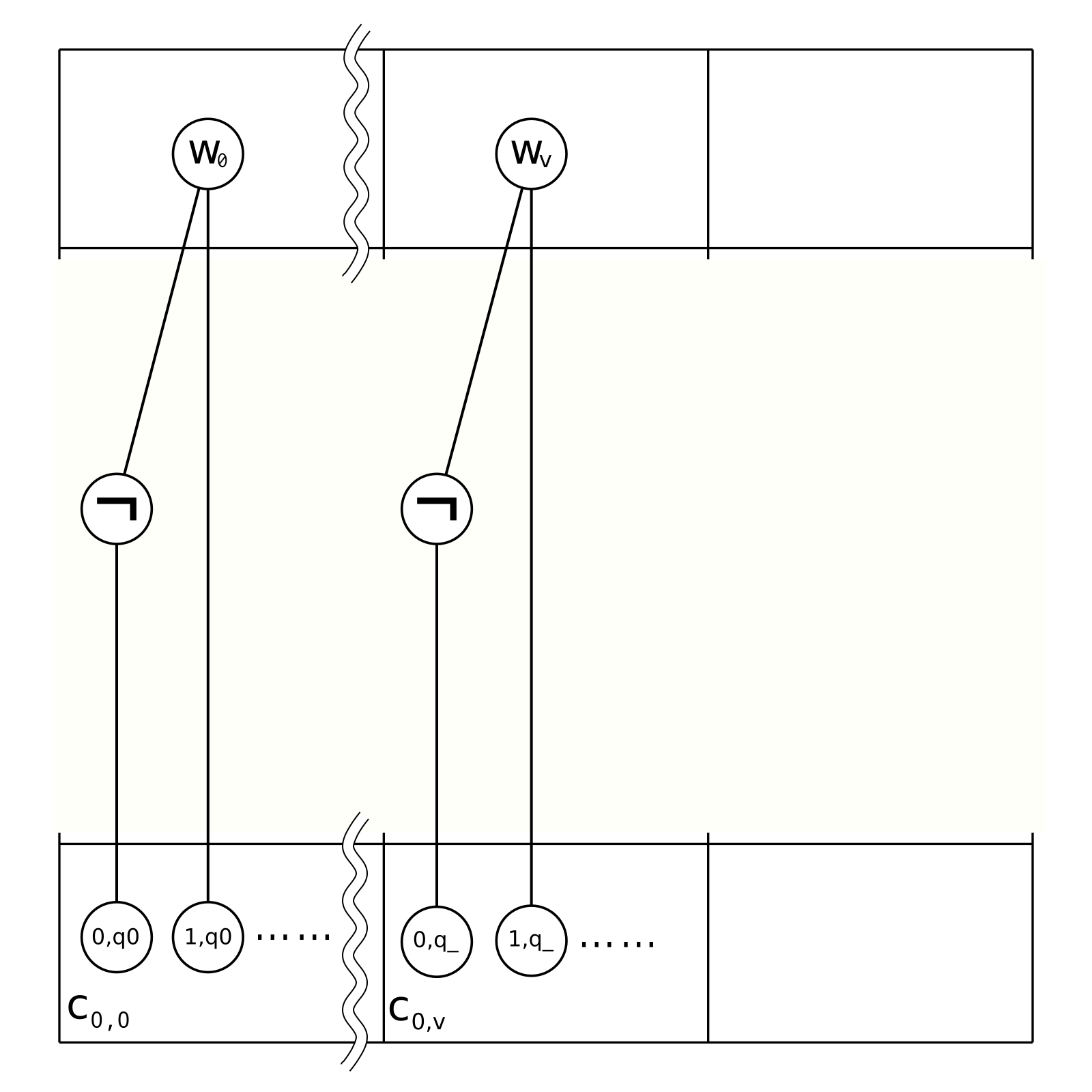
This Proof is based on [Sipser] theorem 9.30 proof. See [Sipser] for detail.

NNF circuit family can emulate DTM by computing every step’s cell values (and head state if head on the cell). Figure 2.2 shows part of a NNF circuit block diagram.

Input of this circuit is modified $w_{1}\cdots w_{n}$ to $c_{1,1}\cdots c_{1,n}$ , and finally output result at $c_{out}=c_{t\left(n\right),1}$ cell. This circuit emulate DTM behavior, so $c_{u,v}$ compute cell’s state of step $u$ from previous step cell $c_{u-1,v}$ and each side cells $c_{u-1,v-1},c_{u-1,v+1}$ (because head affect at most side cells in each step).

Figure 2.3 shows example of $c_{u,v}$ sub circuit that transition function is “if state is $q_{k}$ and tape value is $0$ , then move $+1$ and change state to $q_{m}$ ”. This circuit shows one of transition configuration which $\left(c_{u-1,v-1},c_{u-1,v},c_{u-1,v+1}\right)=\left(q_{k}0,q_{-}0,q_{-}0\right)$ . $q_{-}$ means “no head on the cell”.

Each OR-gate $\vee_{w,q}$ in $c_{u,v}$ correspond to every step’s cell condition (cell value $w$ , and head status $q$ if head exist on the $c_{u,v}$ cell), and output 1 if and only if $c_{u,v}$ cell satisfy corresponding condition. Previous step’s $\vee$ output in $c_{u-1,v-1}$ , $c_{u-1,v}$ , $c_{u-1,v+1}$ are connected to next step’s AND-gate $\wedge_{\delta}$ in $c_{u,v}$ with transition wire. Each $\wedge_{\delta}$ correspond to transition function $\delta$ , and each $\wedge_{\delta}$ output correspond to each transition function’s result of $c_{u,v}$ . To simplify, NNF circuit include separate three gates $\wedge_{\delta,-1}$ , $\wedge_{\delta,0}$ , $\wedge_{\delta,+1}$ according to head exists position $c_{u-1,v-1}$ , $c_{u-1,v}$ , $c_{u-1,v+1}$ , and special transition function $\delta_{-}$ which correspond to no head transition (keep current tape value). So $\wedge_{\delta}$ in $c_{u,v}$ output 1 if and only if previous step’s $\vee$ output in $c_{u-1,v-1}$ , $c_{u-1,v}$ , $c_{u-1,v+1}$ satisfy transition function $\delta$ condition. Each transition functions affect (or do not affect) next step’s condition, so $\wedge_{\delta}$ output is connected to $\vee_{w,qm}$ in $c_{u,v}$ and decide $c_{u,v}$ condition. Because DTM have constant number of transition functions, NNF can compute each step’s cell by using constant number of AND-gates and OR-gates (without NOT-gate).

First step’s cells are handled in a special way. Input is $\left\{0,1\right\}^{*}$ and above monotone circuit cannot manage $0$ value. So NNF circuit compute $\left\{0,1\right\}^{*}\longrightarrow\left\{01,10\right\}^{*}$ by using NOT-gate.

∎

Corollary 2.3.

NNF circuit family can compute P problem with polynomial number of gates of input length.

Confirm NNF circuit family behavior. We define some term that decide relation of inputs.

Definition 2.4.

We will use the term;

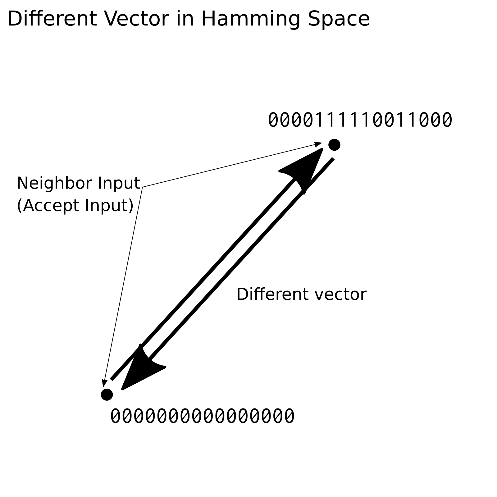
“Neighbor input (pair)” as accept inputs pair that no accept inputs exists between these accept input in Hamming space.

“Boundary input (set) of neighbor input” as reject inputs that exist between neighbor inputs in Hamming space.

“Different variables” as all difference part of values in neighbor input pair.

“Different vector” as vector and inverse vector pair which start and end point is neighbor input pair in Hamming space. To simplify, we use $\overline{1}=-1$ .

“Neighbor distance” as different vector length.

“Sandwich structure” as connected graph which nodes are accept inputs in Hamming space.

Figure 2.5 shows example of sandwich structure which neighbor input pair is $0000111110011000$ and $0000000000000000$ . In this case, $\_\_\_\_11111\_\_11\_\_\_$ and $\_\_\_\_00000\_\_00\_\_\_$ are different variables, and $\left(0000111110011000\right)$ and $\left(0000\overline{1}\overline{1}\overline{1}\overline{1}\overline{1}00\overline{1}\overline{1}000\right)$ are different vector, neighbor distance is 7.

“Effective circuit of accept input $t$ ” as one of minimal sub circuit in NNF circuit that decide circuit output as 1 with accept input $t$ . Effective circuit do not include gates which output 0, or even if these gates change output 0 and effective circuit keep output 1.

Figure 2.7 shows example of effective circuit which circuit is 2.1 and input is $\left\{x_{1},x_{2},x_{3}\right\}=\left\{1,1,0\right\}$ . Dotted gates do not affect OUTPUT-gate even if the gate negate output, so effective circuit do not include them.

Theorem 2.5.

All input variable pair of different variables join at OR-gate in effective circuit.

Proof.

Because all input variable pair is $\left\{01,10\right\}$ and do not include $11$ in every input. NNF circuit is almost monotone circuit, so effective circuit have to to join another accept input $\left\{01,10\right\}$ at OR-gate to connect OUTPUT-gate. ∎

Figure 2.8 shows example of effective circuit which circuit is 2.1 and input are $\left\{x_{1},x_{2},x_{3}\right\}=\left\{1,1,0\right\},\left\{0,0,1\right\}$ . Effective circuit include one of input variable pair, and other side of variable pair do not become 1 in same input. So AND-gate cannot meet another effective circuit.

Theorem 2.6.

NNF circuit have at least one unique AND-gate which correspond to different vector to differentiate neighbor input and boundary input.

Proof.

Mentioned above 2.5, all accept input variable pair of different variables join at OR-gate. Because NNF circuit is almost all monotone circuit, there are a) b) case to join effective circuits;

a) some partial different variables meet at AND-gate, and join at OR-gate these AND-gate output, and meet at AND-gate all OR-gate output. (see 2.8)

b) all different variables meet at AND-gate, and join at OR-gate after meeting AND-gate. (see 2.9)

Case a), because no boundary input become accept input, some OR-gate which join different variables become 0 if input is boundary input (2.8 1,2). That is, effective circuit become 0 if some of these OR-gate become 0, and become 1 if all of these OR-gate become 1. Therefore, it is necessary that effective circuit include AND-gate (2.8 3) that meet all these OR-gate which join all different variables. Such AND-gate become 1 if and only if input include different variables of one side of neighbor input pair. Each pair of different variables correspond to different vector, so the AND-gate correspond to different vector.

Case b), some AND-gate become 1 if and only if input include one side of different variables. Therefore, trunk of these AND-gate (2.9 4,5) does not become 1 if input AND-gate does not include these different variables. Each pair of different variables correspond to different vector, so the AND-gate correspond to different vector.

Therefore, NNF circuit have at least one unique AND-gate that correspond to different vector to differentiate neighbor input and boundary input. ∎

NNF circuit can emulate DTM in polynomial size, and NNF circuit include unique AND-gate that correspond to different vector. Therefore, we can measure problem complexity by counting different vector in problem’s sandwich structure.

3. Negation HornSAT

Consider different vector in actual problems. Let consider Negation HornSAT problem $\overline{HornSAT}$ . $\overline{HornSAT}$ can delete some negative literal which correspond definite clauses. This means that each $\overline{HornSAT}$ accept input are close each other in Hamming space. In fact, we can close neighbor distance within constant distance by devising $\overline{HornSAT}$ description.

Definition 3.1.

We will use the term $\overline{HornSAT}$ as problem if and only if Horn CNF is $\bot$ .

In $\overline{HornSAT}$ , we use special description as following;

$x_{i}$ : Variables in $\overline{HornSAT}$ . $i$ in $x_{i}$ is variable code, and $x$ in $x_{i}$ is constant code. Negative literal $\overline{x}$ is constant code which length is same as $x$ .

$\bot_{i}$ : Disabled Variables in $\overline{HornSAT}$ that $\bot_{i}=\bot$ . $\bot$ in $\bot_{i}$ is constant code which length is same as $x$ .

$-$ : Ignored filler code in $\overline{HornSAT}$ .

All another symbol $\wedge\vee()$ are also constant length code which is same as $x$ .

Theorem 3.2.

In $\overline{HornSAT}$ , there is some sandwich structure which neighbor distance is at most constant size, and number of different vector is at most polynomial size.

Proof.

Let $t=x_{i}\wedge\left(\overline{x_{i}}\vee\cdots\right)\wedge\cdots\in\overline{HornSAT}$ . can reduce another $t^{\prime}=x_{i}\wedge\left(\bot_{i}\vee\cdots\right)\wedge\cdots\in\overline{HornSAT}$ because we can delete all literal $\overline{x_{i}}$ by using definite clauses $x_{i}$ . Neighbor distance between $t,t^{\prime}$ is constant because difference between $\overline{x_{i}}$ and $\bot_{i}$ is constant part of $x,\bot$ . Because all $\bot_{i}=\bot$ , we can reduce all $\bot_{i}\rightarrow\cdots\rightarrow\bot_{-}\rightarrow\bot$ by overwriting $-$ at most constant size in each steps, and each neighbor distance are at most constant. That is, we can reduce $t^{\prime}$ to $t^{\prime\prime}=x_{i}\wedge\left(\bot\vee\cdots\right)\wedge\cdots\in\overline{HornSAT}$ with overwriting constant distance.

The other hand, we can apply above steps all reduction of negative literals. When some clauses have no variables like $\left(\bot\vee\cdots\vee\bot\right)$ , we can overwrite any code in formula because the formula is $\bot$ . Therefore, all of $\overline{HornSAT}$ have neighbor input that distance is at most constant.

Consider number of $\overline{HornSAT}$ different vectors. Let different distance is constant $k$ . Because different distance is $k$ , number of different vector is combination of different variables $\left(\begin{array}[]{c}n\\ k\end{array}\right)$ and combination of variables pair in constant code $2^{k}$ .

$\left(\begin{array}[]{c}n\\ k\end{array}\right)\times 2^{k}=\frac{n!}{k!\times(n-k)!}\times 2^{k}\leq O\left(n^{k}\right)$

Therefore we obtain theorem. ∎

4. Design high complexity problem

Consider designing high complexity problem. Mentioned in this paper, computational complexity correspond to problem structure in Hamming space, especially number of different vector. Therefore, we can design high complexity problem by designing high cardinal number of different vector.

We use Almost perfect nonlinear function (APN function)[Dobbertin] to design high cardinal number of different vector in $F_{2^{n}}$ vector space. APN function $f$ is;

Different function: $f_{a}:F_{2^{n}}\ni x\mapsto f\left(x+a\right)-f\left(x\right)\in F_{2^{n}}$

and $x$ that $f_{a}\left(x\right)=b$ ( $b$ : constant) are at most 2.

In this case, $f_{a}\left(x\right)=f\left(x+a\right)-f\left(x\right)$ is different vector of $f\left(x+a\right)$ and $f\left(x\right)$ , so APN function $f$ have many different vector which number is half of $x$ .

Definition 4.1.

We will use the term;

“ $APNR$ ” as problem with input $w$ , input length $\left|w\right|$ , APN function $f$ ;

$w=uv$ , $\left|u\right|=\left|v\right|$ , $f\left(u\right)=v$

Theorem 4.2.

$APNR\in PH$

Proof.

We can compute $APNR$ with constant alternating Turing Machine (ATM) by computing following way.

(1)

Select minimal polynomial $g\left(x\right)$ as existence.
(2)

Check polynomial solution $\alpha$ as following;
Reject $w$ if $\alpha^{2^{d}-1}\neq 1$ .
Select $\alpha^{r}$ ( $0<r<2^{d}-1$ ) as universal, and reject $g\left(x\right)$ if $\alpha^{r}=1$
(3)

Construct ANR function $f\left(x\right)$ by using $g\left(x\right)$ and APN power functions, and if $f\left(u\right)=v$ then accept $w$ .

We can compute above procedure in polynomial step with constant alternation. So $APNR\in PH$ . ∎

Theorem 4.3.

$APNR$ have $2^{\left|u\right|-1}$ number of different vector.

Proof.

$APNR$ different vector $w_{p}+w_{q}$ ( $w_{p}=u_{p}v_{p}$ , $w_{q}=u_{q}v_{q}$ ) is;

$w_{p}+w_{q}=\left(u_{p}+u_{q}\right)\left(v_{p}+v_{q}\right)$

$=\left(u_{p}+u_{q}\right)\left(f\left(u_{p}\right)+f\left(u_{q}\right)\right)$

Because APN function definition, $u_{p}+u_{q}=a$ then there are at most 2 $\left(u_{p},u_{q}\right)$ that $f\left(u_{p}\right)+f\left(u_{q}\right)=b$ . That is, even if different vector $u_{p},u_{q}$ become same, there are many different vector $f\left(u_{p}\right)+f\left(u_{q}\right)$ which depend on $u_{p}=u_{q}+a$ value.

Therefore, $APNR$ have many different vector that depend on $u$ value, and number of $APNR$ different vector is $2^{\left|u\right|-1}$ . ∎

References

[Sipser] Michael Sipser, (translation) OHTA Kazuo, TANAKA Keisuke, ABE Masayuki, UEDA Hiroki, FUJIOKA Atsushi, WATANABE Osamu, Introduction to the Theory of COMPUTATION Second Edition, 2008
[Ajtai] Ajtai, M. Komlós, J. and Szemerédi, E.: An 0(n log n) sorting network, STOC(1983).
[Furst] Furst, M. Saxe, J.B. and Sipser, M.: Parity, circuits, and the polynomial-time hierarchy Mathematical Systems Theory(1984)
[Razborov] Razborov, A.: Lower bounds on the monotone complexity of some Boolean functions. Mathematics of the USSR(1985)
[Dobbertin] Dobbertin, H.: H. Dobbertin, Almost perfect nonlinear functions on $GF\left(2^{n}\right)$ : the Niho case, Information and Computation 151, (1999).