+jet production via gluon fusion at the LHC
Abstract
Pair production of bosons in association with a hard jet is an important background for Higgs particle or new physics searches at the LHC. The loop-induced gluon-fusion process contributes formally only at the next-to-next-to-leading order. Nevertheless, it can get enhanced by the large gluon flux at the LHC, and thus should be taken into account in relevant experimental searches. We provide the details and results of this calculation, which involves the manipulation of rank-5 pentagon integrals. Our results show that the gluon-fusion process can contribute more than to the next-to-leading order QCD result and increases the overall scale uncertainty. Moreover, interference effects between Higgs and non-Higgs contributions can become large in phase-space regions where the Higgs is far off-shell.
Keywords
Bosons, Standard Model, Hadronic Colliders1 Introduction
The Large Hadron Collider (LHC) is presently running with a center-of-mass energy of 8 TeV and instantaneous luminosity surpassing already the Fermilab’s Tevatron, with the possibility of being upgraded to the designed value, i.e., 14 TeV and , in 2014 [1]. The unprecedented high collision energy and luminosity are necessary for discovering Higgs particles and new physics beyond the Standard Model (SM). However, the higher the collision energy the more complex event topologies get involved. In particular, hadron collision events with multiple hard particles and large jet multiplicities deserve a careful treatment.
In this paper, we investigate production at the LHC, leading to the following event topologies
| (1) |
This process thus contributes for example as background to Higgs + jet production with Higgs decays into Z boson pairs, or slepton pair + jet production with slepton decays into lepton and the lightest super-symmetric particle (LSP). The next-to-leading order (NLO) QCD calculation of the corresponding parton level processes at tree level
| (2) |
has been performed in Refs. [2, 3] without subsequent decays. The resulting QCD corrections are significant (e.g., the K factor is about 1.4 for GeV at the 14 TeV LHC) and reduce the scale uncertainty significantly.
On the other hand, the IR-safe part of the higher-order QCD corrections, i.e. the loop-induced gluon-fusion (GF) process
| (3) |
which formally is of the next-to-next-to-leading order (NNLO), can be enhanced by the large gluon flux at the LHC, as already shown in previous comparative studies [4] on vector boson () pair productions via GF or collision, i.e.
| (4) |
A similar study for the boson case shows contributions of about 10 percent to the next-to-leading order QCD result [5]. Recently, also a study of the GF process appeared, but neglecting the Higgs contributions [6].
Moreover, the GF process (3) corresponds to part of the real emission contributions of the NLO QCD corrections to the loop-induced pair production via GF and thus may be crucial in reducing the theoretical uncertainty for a precise measurement of boson pair production, and also for the inclusive Higgs search via [7].
Based on the above mentioned motivations, we are reporting in this paper on the calculation and results of the GF process (3) at the 7, 8 and 14 TeV LHC11 1 As for the 1.96 TeV Tevatron we have checked that the GF production rates are tiny ( 1% of the NLO QCD ones) due to the small gluon flux and is thus not discussed here.. We, therefore, omit GF production channels with quarks in the initial and final state since they interfere with the LO contributions already at NLO 22 2 The interference effects of production via GF with the LO contribution has been computed in [3] and are below 1%. Furthermore, since we are mostly interested in the effects of the integrated cross section of production in GF, which is not sensitive to the decays, in accordance with Ref. [3], the leptonic decay of the Z bosons and off-shell effects, e.g. , are not considered. The paper is organized as follows. In section 2 we describe the calculation. In section 3 we present numerical results and their discussion. Finally we conclude in section 4.
2 Calculation
We have implemented two independent Monte Carlo programs which rely on different approaches. Cross checks have been performed at the amplitude level for fixed phase-space points and also for integrated cross sections, getting agreement at the double-precision level and within statistical errors, respectively.
The relevant one-loop Feynman diagrams and amplitudes for the partonic process are shown in Fig. 1.

The diagrams are grouped in 4 topological classes. The two diagrams in the upper row correspond to continuum production of the two bosons, either via a pentagon or via a box diagram. The two diagrams in the bottom row both involve a, possibly virtual, Higgs boson, which then decays into a pair. This is mediated by either box or triangle graphs. The Higgs mass dependence of the latter ones and interference effects between Higgs and continuum diagrams will be discussed in Sec. 3.
For program 1, the Feynman amplitudes are generated with FeynArts 3.5 [9] and then manipulated with FormCalc 5.3 [10]33 3 Note the naive scheme [11] is employed in FormCalc. The discussion on its validity in practical one loop calculations in anomaly-free theories can be found e.g. in Refs. [12, 13].. The Fortran libraries44 4 The size of the resulting Fortran library for the helicity amplitude evaluation is about 300 Mb. generated with FormCalc are linked with our Monte Carlo integration code for final use. The tensor integrals are evaluated with the help of the LoopTools-2.5 package [10, 14], which employs the reduction method introduced in Ref. [15] for pentagon tensors up to rank 4, and Passarino-Veltman reduction for the lower point ones up to boxes [16]. In our case rank-5 pentagon tensor integrals are needed in addition, as can be inferred from the fact that the 5 external particles are all vector bosons. We thus have modified LoopTools-2.5 to implement the reduction method for pentagon tensor integrals up to rank 5 as proposed in Ref. [17]. Finally, the resulting regular scalar integrals are evaluated with the FF package [18]. The UV and IR divergent scalar integrals have already been encoded into this version of LoopTools within dimensional regularization, which we have explicitly cross-checked against QCDloop [19].
Although the reduction procedure in Ref. [17] can avoid inverse Gram determinants of external momenta in the reduction step from 5-point to 4-point integrals, the reduction of lower-point tensor integrals cannot within the Passarino-Veltman algorithm. The problem is more severe in our case which involves squared loop amplitudes.
To improve the numerical stability problem due to vanishing Gram determinants further modifications have been made. First, we have implemented in LoopTools the so called ‘Alternative Passarino-Veltman reduction’ for triangle and box tensor integrals, as introduced in Ref. [17], which changes the calculating order of tensor coefficients and results in better numerical convergence behavior than the conventional Passarino-Veltman reduction. Second, we have imposed a jet-measure-like cut to simply cut away a small dangerous region in phase space to avoid numerical problems. The total contribution of this region will turn out to be small.
| (5) | |||
| (6) |
where run over the final state particles. Here is the rapidity and is the azimuthal angle around the beam direction. In Sec. 3, we will discuss the dependence on the choice of .
The program 2 is based on the structure of the Monte-Carlo program Vbfnlo [20]. We use the effective current approach [21], which allows us to compute only four master Feynman diagrams, corresponding to the diagrams appearing in Fig. 1. This calculation is performed with the in-house framework described in Ref. [22], which uses Mathematica [23] and FeynCalc [24]. We use generic vertices split into left- and right-handed components such that every physically allowed permutation can be constructed by contracting with the corresponding effective polarization vectors, which have been multiplied with the electroweak couplings beforehand. Each of the diagrams is split into a vector and an axial-vector part by isolating the contributions. This allows to apply Fury’s theorem independently for the vector and axial-vector components reducing the total number of diagrams to be computed by a factor two. Additionally, for each of the master diagrams, we build Ward identities replacing the generic vertices by their corresponding momenta. This allows us e.g. to reduce analytically a pentagon of rank five into a difference of two boxes and a remainder pentagon of rank four
| (7) |
where means that the corresponding vertex has been replaced by its momentum . The remainder, in this case the pentagon , vanishes for massless propagators and purely vectorial couplings (gluon, photon) for the given contraction. These simplified analytical expressions are used to control the numerical accuracy of the code. We compare numerically the values given by the analytically simplified expressions with the master diagrams, where the polarization vector has been replaced by the corresponding four-momentum. We construct all possible Ward identities for each diagram and physical permutation, e.g. all five different ones for the pentagon before. The deviation is then defined as absolute value of one minus the ratio between the numerically contracted and the analytically calculated diagram. Where more than one Ward identity is possible, we take the largest value. A point is identified as unstable when this value exceeds a given global value . In this case, the complete phase-space point is rejected and the amplitude set to zero. The dependence of the cross section on the required accuracy will be shown in the numerical analysis in the next section.
To reduce the CPU impact of the calculation of these identities, we factorize out the part that depends on the effective currents and the couplings, such that the loop dependent part, including these identities, is only computed for one helicity combination and re-used for the other ones. This reduces the time needed for the additional combinations by about a factor four. Nevertheless, for the final results we apply random helicity summation to sample more phase-space points. For the numerical evaluation of the tensor integrals, we apply the Passarino-Veltman approach of Ref. [16] up to boxes, and for a numerically stable implementation of five-point-coefficients we use the Denner-Dittmaier scheme laid out in Ref. [17] with the set-up and notation of Ref. [22]. Color factors have been computed by hand and cross-checked with the program Color [25].
Additionally, we have implemented a two-layer rescue system for phase-space points where the Ward identities of Eq. (7) are not satisfied. In the first step, we calculate the diagram again using dedicated subroutines for small Gram determinants. These involve the evaluation of three- and four-point functions up to Rank 11 and 9, respectively, following the notation of Ref. [22]. If at this point the Ward identities are still not satisfied, we perform the second step of the rescue system. Here the scalar integrals and tensor reduction routines are evaluated in quadruple precision. This requires reconstructing the external momenta in quadruple precision, so that global energy-momentum conservation is still fulfilled at the higher numerical accuracy while keeping external particles on their mass-shell. This is a crucial step for obtaining an improved behavior of the quadruple precision routines. These routines are only a factor 2-3 slower than the double precision ones, in contrast to the 10-20 factor one would obtain using quadruple precision for the complete diagram, thus reducing significantly the overall slowing factor of the rescue system. With this system we find the percentage of phase-space points that does not pass the Ward identities for a requested accuracy of is completely negligible, see Table 1. The additional CPU time required is below 10% for this accuracy. A detailed discussion of the numerical impact is postponed to the following section.
Furthermore, in this approach the cut of Eq. (5) is not needed to obtain stable results since singular points are correctly identified by the Ward identities. Nevertheless, we have implemented the cut for comparing with program 1. Final results will be given with program 2 without imposing the cut and activating the two rescue systems demanding a global accuracy of the Ward identities of .
In both programs, we have checked the cancellation of UV and IR divergences in our calculations.
3 Numerical Results
In this section, we present the integrated cross sections and differential distributions for production at the LHC with a center-of-mass energy of 7, 8 and 14 TeV. We impose the following set of cuts
| (8) |
to identify massless partons with jets.
We set the top quark mass to GeV, the bottom quark mass to GeV, and the other light quark masses to zero. In accordance with Ref. [3], we set explicitly
| (9) |
We use a constant Higgs width and the default Higgs mass is chosen to be GeV. Results for and GeV will also be shown. The corresponding Higgs decay widths are obtained by HDECAY [26]:
| (10) |
for and GeV, respectively. Throughout our calculation, production rates via GF are calculated with CTEQ6L1 parton distribution functions (PDFs) [27] with the default strong coupling value using the implementation in LHAPDF [28]. Our canonical choice for the renormalization and factorization scales is .


In program 2, we use Ward identities to identify problematic configurations and use a two-layer rescue system. In Fig. 2, we present the cross section for different values of the demanded accuracy . We show results without applying any rescue system as well as the one including only the small Gram determinant expansion and where both this and quadruple precision for scalar and tensor integrals have been switched on.
| Accuracy | before step 1 | after step 1 | after step 2 | ||||||
|---|---|---|---|---|---|---|---|---|---|
| failure rate | failure rate | failure rate | |||||||
| 16. | 8 % | 285.0(4) | 11. | 1 % | 295.3(4) | 0. | 036% | 320.4(4) | |
| 9. | 9 % | 301.8(4) | 5. | 7 % | 307.8(4) | 7. | % | 321.3(4) | |
| 5. | 7 % | 311.1(4) | 2. | 9 % | 315.0(4) | 1. | % | 320.6(4) | |
| 3. | 1 % | 316.2(4) | 1. | 5 % | 317.4(4) | 3. | % | 320.6(4) | |
| 1. | 7 % | 318.1(4) | 0. | 75 % | 319.6(4) | 1. | % | 321.0(4) | |
| 0. | 94 % | 319.3(4) | 0. | 39 % | 320.5(4) | 1. | % | 321.5(4) | |
| 0. | 54 % | 319.6(4) | 0. | 20 % | 320.5(4) | 0 | 320.9(5) | ||
| 0. | 30 % | 320.5(4) | 0. | 10 % | 321.3(4) | 0 | 321.0(6) | ||
| 0. | 19 % | 321.2(5) | 0. | 048 % | 320.8(4) | 0 | 320.6(5) | ||
| 0. | 12 % | 320.8(4) | 0. | 026 % | 321.9(5) | 0 | 322.9(9) | ||
One can see that for an accuracy of the Ward identity test above the double precision results both with and without the dedicated tensor integrals for small Gram determinants agree with the quadruple precision ones better than 1. This agreement is better than one would naively expect if all rejected points contributed with the same average value to the integrated cross section as the accepted ones. In this case, the cross section corrected for the missing phase-space points can be estimated as , where and are the relative rate of failed points and the output of the cross section obtained with the Monte-Carlo program, respectively, given in Table 1. With this prescription one obtains corrected cross sections which increasingly exceed the quadruple precision results as we go to smaller values of the gauge test parameter . This reflects the fact that the rejected points do not belong to any particular enhanced region of the phase-space.
On the other hand, it is clearly visible that the rescue system for small Gram determinants does not solve the problem of the instabilities. This is due to the fact that for a given phase space point for which the Ward identity is not satisfied with the demanded accuracy, there is always some physical permutation that involves not only small Gram determinants but also small Cayley determinants and , so that the expansion breaks down. Note, also, that our Ward identity check is very restrictive since we do not check whether the resulting diagram gives a numerically relevant contribution to the whole event, i.e, a global gauge check demanding the same accuracy will probably result into smaller failure rates since most of the configurations for which the Ward identity is not satisfied contribute little to the whole event. This can be inferred seeing the nice convergence to the right result even allowing deviations of the Ward identities of two orders of magnitude, .
Nevertheless, we have not investigated this further, and, instead, to solve the problem, we change to quadruple precision, which is now also supported in the latest version of gfortran and has a small impact in terms of CPU time in our program. After this step, the instabilities fall well below the per mille level for an accuracy of the Ward identity gauge test of despite the fact of only using quadruple precision for the scalar and tensor integrals. The small fraction of failed points left after this step points to the fact that the loss of precision is really due to the presence of small Gram determinants. Note also that when allowing large deviations of the Ward identities of three orders of magnitude, , some of the runs already start to feel the instabilities, which translates into large weights yielding larger cross sections and statistical errors. Without applying the Ward identities, , most of the runs with different random number seeds simply give arbitrarily huge values with corresponding huge error bars, if not initialized with an optimized grid. In the following, we stick to the set up to switch on the rescue system for an accuracy of the Ward identity of . The CPU cost is at the 10 level even with the poor success rate of the first step, which we keep for academic reasons.

As mentioned in Sec. 2, for program 1 we employ for simplicity to avoid the problem of numerical instability from vanishing Gram determinants. We show in Fig. 3 the dependence of the integrated cross section for production via GF with the cuts of Eq. (8) at the 14 TeV LHC for a Higgs mass of GeV. For both programs the speed of the code is about 4 CPU days on a state-of-the-art computer with the statistical error on the Monte Carlo integration better than 2 per mille. In the region of GeV, all the points agree well with each other within statistical errors, which shows that the dependence is small. However, for smaller GeV, the statistical errors on program 1 are hard to improve further, as expected, and the percentage of runs that gives nonsensical results using different initial seeds increases for decreasing values of the cut. With increasing GeV, deviations from the small limit start to show up and become apparent as the phase space is reduced more and more. In the following, we use program 2 without applying any for the numerical results.
| 7 TeV LHC / | GeV | GeV | GeV | GeV | GeV |
|---|---|---|---|---|---|
| 53.08(8) | |||||
| 8 TeV LHC / | GeV | GeV | GeV | GeV | GeV |
|---|---|---|---|---|---|
| 79.1(1) | |||||
| 14 TeV LHC / | GeV | GeV | GeV | GeV | GeV |
|---|---|---|---|---|---|
| 354.5(2) | |||||
In Tables 2, 3 and 4, we present production rates via GF with on-shell bosons at the 7 TeV, 8 TeV and 14 TeV LHC, for =120, 126, 140, 200 and 400 GeV, respectively. The results for Higgs masses different from 126 GeV are included to demonstrate the effect of interference effects for these masses. While we know from the experimental searches [29, 30] that a Higgs boson with SM coupling strength is not possible there, one with reduced couplings, e.g. the CP-even partner in a Two-Higgs-doublet model, is still viable.
gives the integrated cross sections including both Higgs signal () and continuum () contributions. For , the Higgs contributions are small compared to continuum production, as the intermediate Higgs is far off-shell. Note that we only consider production of on-shell bosons, which is the dominant region for the continuum contribution, where we will focus on in the current work. We see that for Higgs masses below the threshold, which includes the actually observed mass, there is a strong destructive interference between the continuum and the Higgs diagrams. This leads to integrated cross sections which are even below the continuum-only result. Compared to the naive sum, the full result is reduced by roughly 20%. In contrast for Higgs masses above the threshold, interference effects are small and reach at most 4%.

Fig. 4 shows the dependence on the renormalization and factorization scales () of the gluon-fusion production rates at the 14 TeV LHC. The scale dependence is rather large. Varying the scale by a factor 2 downwards (upwards), the cross sections change by 54.2% (-32.5%), 59.4% (-34.4%) and 54.2% (-32.4%) for continuum diagrams, Higgs diagrams and the full result, respectively. Comparing these numbers with the NLO results for the continuum calculated in Ref. [3], the continuum gluon-fusion result gives an additional 9.7% contribution to the cross section at the central scale (13.2% compared to the LO cross section). This changes to 13.9% (18.0%) and 7.0% (10.0%) for decreasing and increasing the scale by a factor two, respectively. The total scale uncertainty of the cross section increases from +8% (+13%) and -6% (-11%) for the NLO QCD (LO) result to +12.1% (+17.8%) and -8.4% (-13.5%) for NLO+GF (LO+GF), again varying the scale by a factor two down- and upwards, respectively.

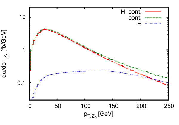
In Fig. 5 we show, in the left-hand panel, the differential cross section for the distribution of the transverse momentum of the jet . Both diagram types lead to increasingly lower cross sections as we go to higher transverse momenta, but the fall-off of the Higgs part is less steep than the continuum part. Compared to the tree-level process [3], the jet distribution here in gluon-fusion is softer due to the dilution effects of the fermion loop. This behavior is consistent with previous findings in Ref. [31] on Higgs+jet production. On the right-hand side of Fig. 5, we present the transverse-momentum distribution of the second Z boson with the smaller value. A similar behavior as for the jet- is observed, and the cross section for the Higgs-only diagrams stays almost constant over a large part of the shown range. For transverse momenta larger than about 200 GeV, it reaches the same order of magnitude as the continuum contribution and even exceeds the combined result.


The origin of this behavior can be understood by looking at the invariant mass of the two bosons shown in Fig. 6. For = 126 GeV in the left-hand panel, the continuum diagrams show a peak directly above the threshold and a fall-off for larger invariant masses. These are dominated by the loop diagrams with massless quarks of the first two generations running in the loop. For the Higgs diagrams in contrast the top-quark loop dominates. Here the peak of the cross section is just above crossing the threshold owing to the P-wave suppression at threshold due to the CP-even nature of the Higgs boson. The Z bosons coming from virtual Higgs decays have larger momenta on average, leading to a harder spectrum. On the right-hand side we show in comparison the same plot, but now setting the Higgs mass to 400 GeV. The Higgs resonance in the ZZ invariant mass spectrum is clearly visible. While for mass values smaller than that constructive interference between the two diagram types appears, it becomes destructive for larger values. This is in particular visible at the large-mass end of the plot, where both contributions have similar size and the sum of the two is about a factor three smaller. Such a behavior has already been observed and explained in production [32]. For large momenta the longitudinal polarizations of the bosons dominate, which for the continuum couple predominantly to the top-quark loop, as does the Higgs. For colliding two on-shell top quarks, unitarity restoration then immediately requires that for the longitudinal polarizations continuum - and -channel diagrams and the -channel Higgs diagram cancel at large invariant masses. This behavior is unchanged when closing the loop and integrating over the loop momentum.


Finally, we display the azimuthal angle separation between the two bosons in Fig. 7. Again, we see a significant difference between the continuum and the Higgs diagrams. In both cases, the two Z bosons are preferably emitted back-to-back, but the effect is more pronounced for the Higgs contribution. This is particularly visible in the right-hand panel, where the differential cross sections are individually normalized to the integrated one.
4 Summary
We have presented a calculation of the loop-induced gluon-fusion process of production at the LHC. Special attention has been paid to the numerical problem of vanishing Gram determinants to obtain stable results.
We have studied distributions of the final-state particles. Here, the contribution of the Higgs diagrams develops larger transverse momenta of the final-state particles. This is due to the crossing of the top-quark pair production threshold, which increases the production for invariant masses above this value. Also, for invariant masses larger than the Higgs mass, destructive interference between Higgs and continuum diagrams appears, leading to a huge reduction of the differential cross section. The effect on the integrated cross section, however, is about 20% for a Higgs mass of 126 GeV and, when compared with the tree-level cross section of -induced ZZj production, small.
Additionally, when compared with the known NLO QCD result, the gluon-fusion part can contribute more than 10% of the NLO QCD cross section, especially at small scales and jet transverse momenta . Moreover, the GF results increase the scale uncertainties of the integrated cross section. For e.g. the benchmark point in Fig. 4, the scale dependence is increased by about a factor 1.5.
Acknowledgements.
This work is supported by the European Community’s Marie-Curie Research Training Network HEPTOOLS under contract MRTN-CT-2006-035505 and the National Natural Science Foundation of China, under Grants No. 11205008. FC and MR acknowledge support by the Deutsche Forschungsgemeinschaft via the Sonderforschungsbereich/Transregio SFB/TR-9 “Computational Particle Physics”, the Initiative and Networking Fund of the Helmholtz Association, contract HA-101(“Physics at the Terascale”), and by the FEDER and Spanish MICINN under grant FPA2008-02878.References
- (1) CERN Press Office, http://press.web.cern.ch/press/PressReleases/Releases2011/PR01.11E.html
- (2) T. Binoth et al., PoS RADCOR2007 (2007) 008 [arXiv:0801.1616 [hep-ph]]; G. Sanguinetti and S. Karg, [arXiv:0806.1394 [hep-ph]]; T. Binoth et al., [arXiv:0807.0605 [hep-ph]].
- (3) T. Binoth, T. Gleisberg, S. Karg, N. Kauer and G. Sanguinetti, Phys. Lett. B 683, 154 (2010) [arXiv:0911.3181 [hep-ph]].
- (4) D. A. Dicus, C. Kao and W. W. Repko, Phys. Rev. D 36 (1987) 1570; E. W. N. Glover and J. J. van der Bij, Phys. Lett. B 219 (1989) 488; E. W. N. Glover and J. J. van der Bij, Nucl. Phys. B 321 (1989) 561; C. Kao and D. A. Dicus, Phys. Rev. D 43 (1991) 1555; T. Matsuura and J. J. van der Bij, Z. Phys. C 51 (1991) 259; C. Zecher, T. Matsuura and J. J. van der Bij, Z. Phys. C 64 (1994) 219 [arXiv:hep-ph/9404295]; K. L. Adamson, D. de Florian and A. Signer, Phys. Rev. D 65 (2002) 094041 [arXiv:hep-ph/0202132]; K. L. Adamson, D. de Florian and A. Signer, Phys. Rev. D 67 (2003) 034016 [arXiv:hep-ph/0211295]; T. Binoth, M. Ciccolini, N. Kauer and M. Kramer, JHEP 0503 (2005) 065 [arXiv:hep-ph/0503094]; T. Binoth, M. Ciccolini, N. Kauer and M. Kramer, JHEP 0612 (2006) 046 [arXiv:hep-ph/0611170]; T. Binoth, N. Kauer and P. Mertsch, arXiv:0807.0024 [hep-ph]; N. Kauer and G. Passarino, JHEP 1208 (2012) 116 [arXiv:1206.4803 [hep-ph]].
- (5) T. Melia, K. Melnikov, R. Rontsch, M. Schulze and G. Zanderighi, JHEP 1208, 115 (2012) [arXiv:1205.6987 [hep-ph]].
- (6) P. Agrawal and A. Shivaji, Phys. Rev. D 86, 073013 (2012) [arXiv:1207.2927 [hep-ph]], and arXiv:1208.2593 [hep-ph].
- (7) R. N. Cahn and M. S. Chanowitz, Phys. Rev. Lett. 56, 1327 (1986).
- (8) J. A. M. Vermaseren, Comput. Phys. Commun. 83 (1994) 45; D. Binosi and L. Theussl, Comput. Phys. Commun. 161 (2004) 76 [arXiv:hep-ph/0309015]; D. Binosi, J. Collins, C. Kaufhold and L. Theussl, Comput. Phys. Commun. 180 (2009) 1709 [arXiv:0811.4113 [hep-ph]].
- (9) J. Küblbeck, M. Böhm, and A. Denner, Comput. Phys. Commun. 60 (1990) 165–180; T. Hahn, Comput. Phys. Commun. 140, 418 (2001) [arXiv:hep-ph/0012260].
- (10) T. Hahn and M. Perez-Victoria, Comput. Phys. Commun. 118, 153 (1999) [arXiv:hep-ph/9807565].
- (11) M. Chanowitz, M. Furman, and I. Hinchliffe, Nucl. Phys. B 159, 225 (1979).
- (12) F. Jegerlehner, Eur. Phys. J. C 18, 673 (2001) [arXiv:hep-th/0005255].
- (13) S. Dittmaier, S. Kallweit and P. Uwer, Nucl. Phys. B 826, 18 (2010) [arXiv:0908.4124 [hep-ph]].
- (14) T. Hahn and M. Rauch, Nucl. Phys. Proc. Suppl. 157, 236 (2006) [hep-ph/0601248].
- (15) A. Denner and S. Dittmaier, Nucl. Phys. B 658, 175 (2003) [arXiv:hep-ph/0212259].
- (16) G. Passarino and M. J. G. Veltman, Nucl. Phys. B 160, 151 (1979).
- (17) A. Denner and S. Dittmaier, Nucl. Phys. B 734, 62 (2006) [arXiv:hep-ph/0509141].
- (18) G. J. van Oldenborgh and J. A. M. Vermaseren, Z. Phys. C 46, 425 (1990), G. J. van Oldenborgh, Comput. Phys. Commun. 66 (1991).
- (19) R. K. Ellis and G. Zanderighi, JHEP 0802, 002 (2008) [arXiv:0712.1851 [hep-ph]].
- (20) K. Arnold et al., Comput. Phys. Commun. 180 (2009) 1661; K. Arnold et al., arXiv:1207.4975 [hep-ph].
- (21) K. Hagiwara and D. Zeppenfeld, Nucl. Phys. B 274 (1986) 1.
- (22) F. Campanario, JHEP 1110 (2011) 070 [arXiv:1105.0920 [hep-ph]].
- (23) Wolfram Research, Inc., Mathematica, Version 5.2, Champaign, IL (2005).
- (24) R. Mertig, M. Bohm and A. Denner, Comput. Phys. Commun. 64, 345 (1991).
- (25) J. Hakkinen and H. Kharraziha, Comput. Phys. Commun. 100 (1997) 311 [hep-ph/9603229].
- (26) A. Djouadi, J. Kalinowski and M. Spira, Comput. Phys. Commun. 108 (1998) 56 [arXiv:hep-ph/9704448]; A. Djouadi, J. Kalinowski, M. Mühlleitner and M. Spira, in J. M. Butterworth et al., Proceedings Les Houches 2009 workshop on TeV colliders, arXiv:1003.1643 [hep-ph].
- (27) J. Pumplin, D. R. Stump, J. Huston, H. L. Lai, P. M. Nadolsky and W. K. Tung, JHEP 0207 (2002) 012 [arXiv:hep-ph/0201195].
- (28) M. R. Whalley, D. Bourilkov and R. C. Group, arXiv:hep-ph/0508110.
- (29) G. Aad et al. [ATLAS Collaboration], Phys. Lett. B 716 (2012) 1 [arXiv:1207.7214 [hep-ex]].
- (30) S. Chatrchyan et al. [CMS Collaboration], Phys. Lett. B 716 (2012) 30 [arXiv:1207.7235 [hep-ex]].
- (31)
R. K. Ellis, I. Hinchliffe, M. Soldate and J. J. van der Bij,
Nucl. Phys. B 297 (1988) 221;
U. Langenegger, M. Spira, A. Starodumov and P. Trueb, JHEP 0606 (2006) 035 [hep-ph/0604156];
Q. Li, M. Spira, J. Gao and C. S. Li, Phys. Rev. D 83, 094018 (2011) [arXiv:1011.4484 [hep-ph]]. - (32) E. W. N. Glover and J. J. van der Bij, Phys. Lett. B 219, 488 (1989) and Nucl. Phys. B 321, 561 (1989).