Stable XOR-based Policies for the Broadcast Erasure Channel with FeedbackThanks: This research has been co-financed by the European Union (European Social Fund – ESF) and Greek national funds through the Operational Program “Education and Lifelong Learning” of the National Strategic Reference Framework (NSRF) – Research Funding Program: Thales. Investing in knowledge society through the European Social Fund. M. Gatzianas was supported by the ERC Starting Project Grant NOWIRE ERC-2009-StG-240317.Thanks: S. Athanasiadou and L. Georgiadis are with the Department of Electrical and Computer Engineering, Division of Telecommunications, Aristotle University of Thessaloniki, Thessaloniki, 54 124, Greece. M. Gatzianas was with the School of Computer and Communication Sciences, EPFL, Switzerland. L. Tassiulas is with the Computer Engineering and Telecommunications Department, University of Thessaly, Volos 38 221, Greece.

Sophia Athanasiadou Marios Gatzianas Affiliation: Leonidas Georgiadis, and Leandros Tassiulas,

Abstract

In this paper we describe a network coding scheme for the Broadcast Erasure Channel with multiple unicast stochastic flows, in the case of a single source transmitting packets to $N$ users, where per-slot feedback is fed back to the transmitter in the form of ACK/NACK messages. This scheme performs only binary (XOR) operations and involves a network of queues, along with special rules for coding and moving packets among the queues, that ensure instantaneous decodability. The system under consideration belongs to a class of networks whose stability properties have been analyzed in earlier work, which is used to provide a stabilizing policy employing the currently proposed coding scheme. Finally, we show the optimality of the proposed policy for $N=4$ and i.i.d. erasure events, in the sense that the policy’s stability region matches a derived outer bound (which coincides with the system’s information-theoretic capacity region), even when a restricted set of coding rules is used.

I Introduction

The information-theoretic capacity region of the Broadcast Erasure Channel (BEC) in the case of one transmitter and $N$ unicast sessions has been recently studied in [1] and [2]. Both of these papers propose coding algorithms based on transmission of linear combinations of packets. These algorithms are shown to achieve capacity in the following settings: 1) $N\leq 3$ and arbitrary channel statistics, and 2) arbitrary $N$ and channel statistics which satisfy certain assumptions (i.e. symmetric channels and one-sided fair channels). However, these schemes are characterized by high complexity (as operations take place in a sufficiently large sized finite field) and decoding delay, since a sufficient number of linear combinations has to be received until a packet is decoded. In [3], we proposed a network coding scheme that overcomes these obstacles by using only XOR operations, generalizing the 2-user network coding scheme in [4] to the case of 3 users. Thus, two low complexity algorithms were proposed, namely XOR1 and XOR2, which additionally had the advantageous property of “instantaneous decodability”. By this term, it is meant that a receiver is able to decode packet $p$ destined for it as soon as it receives an XOR combination of packets containing $p$ . Algorithm XOR2 was proved to achieve capacity for the case of i.i.d. channels as well as spatially independent channels with erasure probabilities that do not exceed 8/9.

However, the system considered in [3] is a saturated system, where a predefined number of packets needs to be transmitted to each user. This model is not frequently encountered in practice. Moreover, algorithms XOR1 and XOR2 cannot be easily generalized to more than 3 users. This happens because, at each time slot, coding choices have to be determined a priori so that each transmission is optimally exploited in terms of allowing multiple users to simultaneously decode their packets as well as create favorable future coding opportunities. However, for $N>3$ , the number of coding choices increases dramatically so that there is no clear intuition on the optimal choice (this will become apparent once the model and queue structure is described).

In the current work, we propose a general network coding scheme for the case of a single transmitter sending packets to $N$ users through the BEC with feedback, generalizing the scheme proposed in [3]. Any packet arriving to the transmitter is initially placed in one of $N$ queues. Depending on the received feedback, these packets (or XOR combinations of them) may travel through a network of queues, before they reach their destination, in order to exploit the overhearing benefit of the broadcast channel. Coding and packet movement rules are imposed in order to ensure instantaneous decodability of packets and better exploitation of coding opportunities.

While in [3] we examined a saturated system, in this paper we consider a stochastic model where packets may arrive randomly at the transmitter at any time slot. Additionally, we use a backpressure type online algorithm that makes each coding choice based on instantaneous quantities, such as queue sizes, without requiring knowledge of future events. Therefore, we do not need to predefine the coding choices (as in [3]), and the proposed network coding scheme can be applied to an arbitrary number of users. For the specific case of 4 users and i.i.d. erasure events, we present a stabilizing policy that uses only a subset of all possible coding choices and prove that the policy stability region coincides with the information theoretic capacity region of the standard BEC with feedback. This result is quite intriguing, considering the restrictions imposed on the policy (XOR operations only, instantaneous decodability, reduced set of coding choices).

The network stability of single hop broadcast erasure channels with feedback has also been examined in [5], which considered broadcast traffic only and investigated the stability regions of plain retransmission and linear network coding schemes (parameterized over the field size) as opposed to a proposed dynamic virtual queue-based policy. The latter policy was shown to be optimal for 2 users while, for $N>2$ and i.i.d. erasures, it achieved a stable rate that differs from the cut-set bound by a factor of $O(\epsilon^{m+1})$ , where $m$ is the number of queue “levels” that participate in the coding decision (see [5] for more details and definitions; $m$ can be loosely regarded as a measure of the encoding complexity) and $\epsilon$ is the erasure probability. Although the structure of the virtual queues and coding rules are inspired by similar concepts as in our work, the actual rules for moving packets between the queues are much more involved in our work since we are interested in achieving the optimal stability region for all values of $\epsilon$ instead of only asymptotic optimality as $\epsilon\to 0$ (these notions of optimality ignore any overhead). An additional cause for rule complexity in our work is the fact that multiple unicast sessions are much more difficult to handle (due to the inherent competition between different sessions) than a single broadcast session. Furthermore, there is no guarantee in [5], for the general case of $N$ users, regarding instantaneous decodability.

The work in [6] studied a network which is described by an underlying complete graph where each edge is modeled as a Markov chain ON/OFF channel (i.e. a generalization of the memoryless erasure channel), while there also exists a special “relay” node with XOR coding capabilities which can overhear all transmissions. Any transmissions to/from the relay are error-free. The work considers multiple unicast flows, originating in all nodes except for the relay, and explicitly accounts for instantaneous decodability by mapping this constraint into a specially constructed conflict graph (a similar graph structure is used in [7] to model the same constraint). It proposes an online backpressure policy that requires computing in each slot the maximum weight independent set of the time-varying conflict graph. Although the work bears similarities to our paper in terms of mathematical techniques and the optimization problem that results, the model is quite different. Hence, the proposed coding policies are quite different and the results in [6] cannot be used to show one of our main results, namely that the proposed scheduling and coding policies achieve channel capacity for BEC with i.i.d. erasures. In particular, the broadcast channel at the relay (which is the only node that can perform XOR coding) is error-free in [6], while we are interested in broadcast erasure channels.

In summary, the contribution of this paper is as follows:

1.

We develop a systematic network-coding-based framework for constructing instantaneously decodable feedback-based XOR coding schemes for the BEC with multiple unicast sessions and an arbitrary number of users. This requires a (highly non-trivial and quite involved) generalization of the rules in [3] and the replacement of the algorithmic core in [3] with a backpressure-type online algorithm proposed in [8], which makes each coding choice based on instantaneous quantities instead of a predefined set of ordered actions. The new policy, which cannot possibly be constructed from [3] through any obvious procedure, is elegant and conceptually simple, considering its general applicability.
2.

We derive an outer bound, for arbitrary $N$ , on the stability region of the network through an elegant flow argument and relate this to a bound on the information-theoretic capacity region of the “extended” BEC channel (where idle slots are allowed).
3.

Finally, for the special case of $N=4$ and i.i.d. erasures across users, we carefully restrict the allowable coding choices and present a stabilizing policy on top of the previous network coding scheme whose stability region is essentially identical to the capacity region of the 4-user system (whereas in 2. above we only relate outer bounds). Hence, we show that XOR combining achieves both instantaneous decodability and throughput optimality in this setting. Considering that the proposed policy uses only a subset of all possible coding choices and only XOR operations, while guaranteeing instantaneous decodability, this result is quite unexpected.

The rest of the paper is organized as follows: in Section II, the system model is introduced along with some useful notation. In Section III, the proposed network coding scheme is described, while in Section IV the applied stabilizing policy is presented. In Section V, an outer bound on the stability region of the system under study is derived. In Section VI, we prove, for the case of 4 users and i.i.d. erasure events, that the stability region of such a system coincides with the capacity outer bound of the standard broadcast erasure channel with feedback. In Section VII we examine some implementation issues while Section VIII concludes the paper. Some technical proofs are contained in the Appendix.

II System model and notation

We describe some notation that will be used in the following. Sets are denoted by calligraphic letters, e.g. $\mathcal{M}$ , and the empty set by $\emptyset$ . The cardinality of set $\mathcal{M}$ is denoted by $\left|\mathcal{M}\right|$ and we write $M=\left|\mathcal{M}\right|$ . Random variables are denoted by capital letters and their values by small case letters. Vectors are denoted by bold letters, e.g. $\boldsymbol{A}=\left(A_{1},\ldots,A_{n}\right)$ . The expected value of a random vector is the vector consisting of the expected values of its components, i.e., $\mathbb{E}\left[\boldsymbol{A}\right]=\left(\mathbb{E}\left[A_{1}\right],\ldots,\mathbb{E}\left[A_{n}\right]\right)$ .

We consider a time-slotted system where slot $t=0,1,\ldots$ corresponds to the time interval $[t,\>t+1).$ The system consists of a base station $B$ and a set $\mathcal{N}=\left\{1,2,\ldots,N\right\}$ of receivers (users). At the beginning of slot $t$ , $A_{i}(t)$ data packets arrive at $B$ with an average rate of $\lambda_{i}=\mathbb{E}\left[A_{i}(t)\right]$ ; these packets must be delivered to receiver $i$ and are referred to as “flow $i$ ” packets, where we denote $\boldsymbol{A}(t)=\left(A_{1}(t),\ldots,A_{N}\left(t\right)\right)$ . All packets consist of $L$ bits, and the transmission time of each packet is $1$ slot. A packet transmitted by $B$ may be either correctly received or completely erased by any receiver (broadcast medium). After each transmission, the receivers send feedback to $B$ (through an error-free zero-delay channel) informing whether the transmitted packet has been correctly received or not (ACK/NACK feedback). We also assume that if no packet is transmitted in a slot (say, because all queues are empty), then all receivers realize that the slot is idle.

Packet arrivals are assumed to be independent and identically distributed across time, but arbitrarily correlated across users. That is, the process $\left\{\boldsymbol{A}\left(t\right)\right\}_{t=0}^{\infty}$ consists of i.i.d. random vectors, while the components of each vector $\boldsymbol{A}\left(t\right)$ may be arbitrarily correlated. Similarly, packet erasures are i.i.d across time and are initially assumed to be arbitrarily correlated across users (we later concentrate on the special case of spatially i.i.d. erasures). The packet arrival and erasure processes are independent. For subsets $\mathcal{S},\mathcal{G}\subseteq\mathcal{N}$ with $\mathcal{S}\cap\mathcal{G}=\emptyset$ , we denote by $P_{\mathcal{G},\mathcal{S}}$ the probability that a transmitted packet is erased at all receivers in $\mathcal{G}$ and received by all receivers in $S$ (no condition is imposed on packet reception or erasure for receivers in $\mathcal{N}-\left(\mathcal{S}\cup\mathcal{G}\right)$ ). We also denote by $\epsilon_{\mathcal{G}}$ the probability that a transmitted packet is erased by all receivers in $\mathcal{G}$ , i.e., $\epsilon_{\mathcal{G}}=P_{\mathcal{G},\varnothing}.$ For simplicity, we slightly abuse the notation and write $\epsilon_{i}$ or $\epsilon_{ij}$ instead of $\epsilon_{\left\{i\right\}}$ or $\epsilon_{\left\{i,j\right\}}$ , respectively.

III Network coding scheme description

III-A Definitions

Exogenous packets arriving at $B$ and being intended for user $i\in\mathcal{N}$ are called “native packets for $i$ ”. A packet is simply termed “native” if it is a native packet for some user (due to the unicast traffic, a packet is native for exactly one user). According to the policies to be described below, all transmitted packets are either native, or XOR combinations of native packets. In other words, any transmitted packet $p$ can be written as $p=\bigoplus_{l=1}^{n}s_{l}$ (where $\oplus$ denotes the XOR operation), where $s_{l}$ are native packets, and we say that “ $p$ contains $s_{l}$ ” or “ $s_{l}$ is contained in $p$ ”, or “ $s_{l}$ is a constituent packet of $p$ ”. As will be seen, it is possible, and actually beneficial, for $p$ to contain native packets for more than one user. To shorten the description in the following, we say that a packet $p$ is an XOR combination of native packets even when $p$ consists of a single native packet. Also, a native packet $q$ for user $i$ is unknown to $i$ at a given time if it has not been decoded by $i$ by that time. The following definitions, which are introduced in earlier work [3], will be crucial in the subsequent analysis.

Definition 1.

User $i$ is a Listener of a packet $p$ iff both of the following conditions are true:

1.

$p$ is an XOR combination of packets, not necessarily native, that $i$ has correctly received.
2.

$p$ contains no native packet for $i$ that is unknown to $i$ . Equivalently, if $p$ contains a native packet $s$ for user $i$ , then the packet $s$ is known to (i.e. has already been decoded by) $i$ .

Definition 2.

User $i$ is a Destination of a packet $p$ iff either $p$ is a native packet for user $i$ that is unknown to $i,$ or $p$ can be decomposed as an XOR combination of the form $p=q\oplus c$ where

1.

$q$ is a native packet for $i$ and unknown to $i,$ and
2.

$i$ is a Listener of $c$ .

We hereafter use the terms Listener, Destination to exclusively refer to the above technical definitions. The decomposition of a packet $p=q\oplus c$ with Destination $i$ alluded to in Definition 2 is unique, since $c$ cannot itself contain an unknown native packet for $i$ , due to the second condition of Definition 1 (since $i$ is also a Listener of $c$ ). Hence, a packet $p$ for which user $i$ is a Destination can contain exactly one unknown native packet $q$ for $i$ , which we denote as $q=p(i)$ (we call $p(i)$ the “unknown native packet” of $i$ in $p$ ). On the other hand, notice that the second condition of the Listener definition does not assert that $p$ always contains a native packet $s$ for user $i$ , only that the existence of such a packet implies that $s$ is known to $i$ . Furthermore, the properties of Destination and Listener are time-dependent since they depend on notions such as “packets known to user $i$ ”, which are inherently time-dependent. Clearly, the Listener property is absorbing, in the sense that if user $i$ is a Listener for packet $p$ at slot $t$ , it remains a Listener for $p$ for all slots $\tau>t$ .

To better understand the previous definitions and some of their fine points, we offer the following illustrative examples:

•

Denote all native packets for users $i,j$ with $\tilde{r},\tilde{s}$ , respectively; we will use indices $\tilde{r}_{1},\tilde{r}_{2},\ldots,$ and $\tilde{s}_{1},\tilde{s}_{2},\ldots,$ to refer to different native packets for the same user. Suppose $p=\tilde{r}\oplus\tilde{s}$ is transmitted, where $\tilde{r},\tilde{s}$ are unknown to $i$ and $j$ , respectively, and have been previously received by $j,i$ , respectively. Then, according to Definition 2, both $i$ and $j$ are Destinations for $p$ . If $p$ is only received by a third user $k$ , then $k$ becomes a Listener for $p$ (since $\tilde{r},\tilde{s}$ are not native packets for $k$ ). If $i$ receives $p$ in the future, then $i$ instantly decodes its native packet $\tilde{r}$ , ceases to be a Destination for $p$ , and becomes a Listener for $p$ , as $p$ no longer contains a native packet of $i$ that is unknown to $i$ .
•

Suppose that $p=\tilde{r}_{l}\oplus\tilde{s}_{l}$ is transmitted and received by $i$ , where neither $\tilde{r}_{l}$ nor $\tilde{s}_{l}$ has been decoded by $i$ in the past. Then, according to Definition 1, $i$ is not a Listener of $p$ (since $p$ contains an unknown native packet $\tilde{r}_{l}$ for $i$ ), even though it knows $p$ . In juxtaposition to the previous example, we note the following subtle point: although a user can only become a Listener of a packet after receiving an XOR combination containing the packet, the previous example shows that it is not always true that every successful reception of a packet by a user automatically makes the user a Listener for the received packet. To take that example one step further, suppose now that $\tilde{p}=\tilde{r}_{m}\oplus p$ is transmitted immediately after $p$ and received by $i$ . Then, $i$ is not a Destination for $\tilde{p}$ (since Definition 2 would require $i$ to be a Listener of $p$ at the time of $\tilde{p}$ ’s transmission) even though $i$ is able to decode $\tilde{r}_{m}$ . Since $\tilde{p}$ is an Innovative packet¹¹ 1 since each transmitted packet $p$ is an XOR combination of native packets, we can write $p$ as $p=\bigoplus_{n}a_{n,p}^{(i)}\tilde{r}_{n}^{(i)}\oplus d_{p}$ , where $\tilde{r}_{n}^{(i)}$ are all native packets for user $i$ , the (composite) packet $d_{p}$ contains no native packet for $i$ and $a_{n,p}^{(i)}\in GF(2)$ are suitable coefficients. Hence, for each transmitted packet $p$ and each user $i$ , we can associate a vector $\mathbf{a}_{p}^{(i)}=(a_{n,p}^{(i)})$ over the field $GF(2)$ and consider the space spanned by the vectors $\mathbf{a}^{(i)}$ that correspond to all packets previously received by user $i$ . Packet $p$ is defined in [9] to be Innovative for user $i$ if the $\mathbf{a}_{p}^{(i)}$ vector is linearly independent w.r.t. the $\mathbf{a}^{(i)}$ vectors of all previously received packets by $i$ . Hence, an Innovative packet essentially brings “fresh” information to a user. for $i$ , we conclude that the notion of “ $i$ is a Destination for $\tilde{p}$ ” is a stronger notion than “ $\tilde{p}$ is Innovative for $i$ ”. As will be seen, the proposed policies ensure that this scenario never occurs; it is mentioned here only to illustrate the Innovative/Destination distinction.

As will be seen, transmitted packets may have several receivers as Destinations or Listeners. The next fact follows from Definition 2.

Fact 1.

If user $i$ is a Destination for a packet $p$ and $i$ receives $p$ , then $i$ is able to immediately (i.e. instantly) decode the unknown native packet intended for it that is contained in $p$ .

Hence, one way of guaranteeing instant decodability in the proposed scheme would be to guarantee that whenever a transmitted packet $p$ contains an unknown native packet for some user $i$ , then $i$ is a Destination for $p$ . This desirable property will be eventually proved once the coding scheme is fully described.

III-B Queue management and coding choices

Under the proposed policies, packets may be placed in various queues at the transmitter side, based on the received feedback. A general queue $Q_{\mathcal{D}}^{\mathcal{L}}$ is characterized by two index sets $\mathcal{L},\mathcal{D}$ satisfying the following criteria:
Compatibility criteria (CC) for sets $\mathcal{L},\mathcal{D}$

1.

$\mathcal{L},\mathcal{D}\subseteq\mathcal{N},$
2.

$\mathcal{L}\cap\mathcal{D}=\emptyset,$
3.

$\mathcal{D}\neq\emptyset,$
4.

$\mathcal{L}=\emptyset$ only if $\left|\mathcal{D}\right|=1$ .

For simplicity, we will denote queue $Q_{\{i,j\}}^{\{k\}}$ by $Q_{ij}^{k},$ and queue $Q_{\{i\}}^{\emptyset}$ by $Q_{i}.$ Also, we use the notation $p_{\mathcal{D}}^{\mathcal{L}}$ to denote a packet that is stored in queue $Q_{\mathcal{D}}^{\mathcal{L}}$ and denote with $\lvert Q^{\mathcal{L}}_{\mathcal{D}}\rvert$ the number of packets stored in $Q^{\mathcal{L}}_{\mathcal{D}}$ . We hereafter assume that all sets $\mathcal{L}$ , $\mathcal{D}$ for queues $Q^{\mathcal{L}}_{\mathcal{D}}$ satisfy the CC and will not state this explicitly.

In addition to the above network of queues, it will be helpful to introduce a network of “virtual” queues $V^{\mathcal{L}}_{\mathcal{D}}(i)$ , for all $\mathcal{L},\mathcal{D}$ and $i\in\mathcal{D}$ as follows: each $V^{\mathcal{L}}_{\mathcal{D}}(i)$ exclusively contains “tokens” identifying native packets, namely the unknown native packets for user $i\in\mathcal{D}$ which are contained in packets stored in $Q^{\mathcal{L}}_{\mathcal{D}}$ . We refer to these tokens as “virtual packets” and write $p^{\mathcal{L}}_{\mathcal{D}}(i)$ to refer both to a token stored in $V^{\mathcal{L}}_{\mathcal{D}}(i)$ as well as to the native packet identified by this token. In the following, we will use the term “packet movement” between virtual queues to actually refer to token movement (tokens are atomic entities so they cannot be further decomposed: each token moves as a unit). Hence, queues $V^{\mathcal{L}}_{\mathcal{D}}(i)$ do not really exist at the transmitter side and should only be examined at a conceptual level, since they will be useful in Sections V, VI. In contrast to the “virtual” network, the queues $Q^{\mathcal{L}}_{\mathcal{D}}$ and the packets stored in them will be referred to as “real”.

We also associate with each queue $Q^{\mathcal{L}}_{\mathcal{D}}$ a group of non-negative integer counters $K^{\mathcal{L}}_{\mathcal{D}}(i)$ , for each $i\in\mathcal{D}$ , which are interpreted as the number of unknown native packets for user $i$ contained in packets stored in $Q^{\mathcal{L}}_{\mathcal{D}}$ (equivalently, the number of tokens for user $i$ in $Q^{\mathcal{L}}_{\mathcal{D}}$ ), i.e. it holds by definition $K^{\mathcal{L}}_{\mathcal{D}}(i)=\lvert V^{\mathcal{L}}_{\mathcal{D}}(i)\rvert$ . We will later prove the important property $K^{\mathcal{L}}_{\mathcal{D}}(i)=\lvert Q^{\mathcal{L}}_{\mathcal{D}}\rvert$ for all $i\in\mathcal{D}$ . Initially, all queues are empty and all counters set to 0.

We classify queues into $N$ levels, where level $w\in\left\{1,\ldots,N\right\}$ contains all queues $Q_{\mathcal{D}}^{\mathcal{L}}$ such that $\left|\mathcal{L}\right|+\left|\mathcal{D}\right|=w$ . Moreover, we classify queues of level $w\geq 3$ into sublevels, where sublevel $w.u$ includes queues of level $w$ with $\left|\mathcal{L}\right|=u$ , $u\in\left\{1,\ldots,w-1\right\}$ . In Figure 1, we give an example of the queue network when $N=3$ .

Refer to caption — Fig. 1: Network of queues for $N=3$ (virtual queues are not shown since they are not used by the transmitter).

Under the proposed scheme, XOR combinations of packets are transmitted, which contain at most one packet from each of the queues $Q_{\mathcal{D}}^{\mathcal{L}}.$ While the specific choice of packets depends on the received feedback and the specific algorithm that is employed, the following rule always holds.

Basic Coding Rule (BCR) A set $\mathcal{P}=\left\{p_{\mathcal{D}_{1}}^{\mathcal{L}_{1}},\ldots,p_{\mathcal{D}_{\nu}}^{\mathcal{L}_{\nu}}\right\}$ of $\nu$ packets, one from each of the different queues $\left\{Q_{\mathcal{D}_{1}}^{\mathcal{L}_{1}},\ldots,Q_{\mathcal{D}_{\nu}}^{\mathcal{L}_{\nu}}\right\}$ , can be combined (by XORing) into a single coded packet only if

\mathcal{D}_{n}\subseteq\mathcal{L}_{r},\;\forall\,r\neq n,\;n,r\in\left\{1,\ldots,\nu\right\}.

(1)

Note that the Basic Coding Rule implies that $\mathcal{D}_{n}\cap\mathcal{D}_{r}=\emptyset$ , for all $r\neq n$ , $n,\>r\in\left\{1,\ldots,\nu\right\}$ . Indeed, $i\in\mathcal{D}_{n}$ implies, through (1), that $i\in\mathcal{L}_{r}$ and, since according to CC it holds $\mathcal{D}_{r}\cap\mathcal{L}_{r}=\emptyset,$ it follows that $i\notin\mathcal{D}_{r}$ .

We have not yet fully specified the criterion according to which a packet is stored in a queue. It will be convenient for packets stored in the same queue to have some common characteristics or properties. Since the notions of Destination/Listener are crucial for keeping track of the packet’s history, we use these two notions as the basis for the packet storage rules. Specifically, we require the following properties to hold:

Basic Properties (BP) of packets stored in queues $Q_{\mathcal{D}}^{\mathcal{L}}$ :

1.

Each packet $p_{\mathcal{D}}^{\mathcal{L}}\in Q_{\mathcal{D}}^{\mathcal{L}}$ is an XOR combination of native packets (including the special case of a single native packet), not necessarily for the same user.
2.

For each packet $p_{\mathcal{D}}^{\mathcal{L}}\in Q_{\mathcal{D}}^{\mathcal{L}}$ , the set of Destinations for $p^{\mathcal{L}}_{\mathcal{D}}$ is $\mathcal{D}$ and all $i\in\mathcal{L}$ are Listeners for $p_{\mathcal{D}}^{\mathcal{L}}$ .
3.

For each packet $p_{\mathcal{D}}^{\mathcal{L}}\in Q_{\mathcal{D}}^{\mathcal{L}}$ , if $p_{\mathcal{D}}^{\mathcal{L}}$ contains an unknown native packet $q$ for some user $i$ , then $i$ is a Destination for $p_{\mathcal{D}}^{\mathcal{L}}$ . Hence, taking BP2 into account, it follows that $i\in\mathcal{D}$ .
4.

For each native packet $q$ for user $i$ that has not been decoded by $i$ yet, there exists exactly one packet $p_{\mathcal{D}}^{\mathcal{L}}\in Q_{\mathcal{D}}^{\mathcal{L}}$ (for some sets $\mathcal{L},\mathcal{D}$ ) such that $q=p_{\mathcal{D}}^{\mathcal{L}}(i)$ , i.e. $p_{\mathcal{D}}^{\mathcal{L}}$ is a composite packet that contains $q$ .

We should stress the following subtle difference in terms of reference between BP1–BP3 and BP4: BP1–BP3 describe properties of packets stored in any queue $Q_{\mathcal{D}}^{\mathcal{L}}$ , while BP4 is an existence statement that essentially describes properties of native packets, which are then related to some queue $Q_{\mathcal{D}}^{\mathcal{L}}$ .

In retrospect, the Basic Properties justify the Compatibility Criteria imposed on $\mathcal{D},\mathcal{L}$ . Specifically, the fact that $\mathcal{D},\mathcal{L}$ contain Destinations and Listeners, respectively, for a packet $p$ implies that $\mathcal{L}\cap\mathcal{D}=\emptyset$ , since $p$ cannot contain any packet that is unknown to a Listener user, due to condition 2 of Definition 1 (hence, a Listener can never be a Destination, although a Destination for a packet becomes a Listener upon reception of the packet). The condition $\mathcal{D}\neq\emptyset$ captures the fact that a packet need only be stored in the queues for as long as it contains an unknown native packet for at least one user. Finally, before any transmissions occur, each native packet has a singleton Destination set and an empty Listener set.

The next result follows immediately from BP.

Lemma 1.

For all $\mathcal{L},\mathcal{D}$ that satisfy CC, BP implies that $K^{\mathcal{L}}_{\mathcal{D}}(i)=\lvert Q^{\mathcal{L}}_{\mathcal{D}}\rvert$ for all $i\in\mathcal{D}$ .

Proof:

We slightly abuse notation and use $Q^{\mathcal{L}}_{\mathcal{D}}$ to refer to the queue indexed by $\mathcal{L},\mathcal{D}$ as well as the set of packets stored in the queue. We also denote with $\mathcal{P}_{i}$ the set of unknown native packets for user $i$ that are contained in packets stored in $Q^{\mathcal{L}}_{\mathcal{D}}$ . By definition, it holds $K^{\mathcal{L}}_{\mathcal{D}}(i)=\lvert\mathcal{P}_{i}\rvert$ , so that it suffices to show $\lvert\mathcal{P}_{i}\rvert=\lvert Q^{\mathcal{L}}_{\mathcal{D}}\rvert$ . Consider any $i\in\mathcal{D}$ ; by BP4, any unknown native packet for user $i$ in $\mathcal{P}_{i}$ is contained in exactly one packet stored in $Q^{\mathcal{L}}_{\mathcal{D}}$ , which implies $\lvert\mathcal{P}_{i}\rvert\leq\lvert Q^{\mathcal{L}}_{\mathcal{D}}\rvert$ . Also, by BP2, any packet $p^{\mathcal{L}}_{\mathcal{D}}\in Q^{\mathcal{L}}_{\mathcal{D}}$ contains exactly one unknown native packet for user $i$ (since $i\in\mathcal{D}$ is a Destination for $p^{\mathcal{L}}_{\mathcal{D}}$ ) and, by BP4, no two distinct packets in $Q^{\mathcal{L}}_{\mathcal{D}}$ can contain the same unknown native packet for $i$ , which implies $\lvert Q^{\mathcal{L}}_{\mathcal{D}}\rvert\leq\lvert\mathcal{P}_{i}\rvert$ . This completes the proof. ∎

The significance of the BP (apart from a systematic way of storing packets in queues) lies in the fact that, combined with BCR, they guarantee the desired instantaneous decodability property, as described in the next result.

Lemma 2.

If BP holds at the beginning of slot $t$ and the transmitted packet $p$ at slot $t$ is created according to BCR, the following statement is true: if $p$ contains an unknown native packet for some user $i$ , then $i$ is a Destination for $p$ . Hence, by Fact 1, any user for which $p$ contains an unknown native packet can instantly decode it upon reception of $p$ .

Proof:

Let the transmitted packet $p=\bigoplus_{k=1}^{\nu}p_{\mathcal{D}_{k}}^{\mathcal{L}_{k}}$ , formed according to BCR, contain some unknown native packet $q$ for user $i$ . Then, $q$ must be contained in one of the $p_{\mathcal{D}_{k}}^{\mathcal{L}_{k}}$ packets that comprise $p$ , say $p_{\mathcal{D}_{k^{\ast}}}^{\mathcal{L}_{k^{\ast}}}$ . BP3 now implies that, since $q$ is unknown to $i$ , $i$ is a Destination for $p_{\mathcal{D}_{k^{\ast}}}^{\mathcal{L}_{k^{\ast}}}$ so that, by BP2, it holds $i\in\mathcal{D}_{k^{\ast}}$ . Hence, we can write $p_{\mathcal{D}_{k^{\ast}}}^{\mathcal{L}_{k^{\ast}}}=q\oplus c$ , where $i$ is a Listener for $c$ . Furthermore, the BCR implies that $i\in\mathcal{L}_{r}$ for all $r\neq k^{\ast}$ , since it holds $i\in\mathcal{D}_{k^{\ast}}$ , so that we can write $p=q\oplus c\oplus\bigoplus_{r\neq k^{\ast}}p_{\mathcal{D}_{r}}^{\mathcal{L}_{r}}$ . By BP2 again, $i$ is a Listener for each $p_{\mathcal{D}_{r}}^{\mathcal{L}_{r}}$ (since $i\in\mathcal{L}_{r})$ , whence it follows that $i$ is a Destination for $p$ . Fact 1 now implies that $i$ can instantly decode $q$ upon reception of $p$ . ∎

Notice that Lemma 2 proves a property which is essentially identical to BP3, albeit for the transmitted packet $p$ only (whereas BP3 holds for all packets stored in queues $Q_{\mathcal{D}}^{\mathcal{L}}$ ). In fact, the previous lemma can be strengthened into the following statement, which specifies the users that can potentially instantly decode unknown native packets after reception of $p$ . This corollary will be crucially used in the proof of subsequent results.

Corollary 1.

If BP holds at the beginning of slot $t$ and the transmitted packet $p$ is created according to BCR, then $p$ contains unknown native packets for all users in $\cup_{k=1}^{\nu}\mathcal{D}_{k}$ , and only for them (in fact, $\cup_{k=1}^{\nu}\mathcal{D}_{k}$ is the set of Destinations for $p$ at the beginning of slot $t$ ). Also, only the users in $\mathcal{S}\cap\left(\cup_{k=1}^{\nu}\mathcal{D}_{k}\right)$ , where $\mathcal{S}$ is the set of users that receive $p$ , can decode any unknown native packets contained in $p$ .

Proof:

We have already shown in the proof of Lemma 2 that if $p$ contains an unknown native packet for some user $i$ , then there exists some $k^{\ast}$ such that $i\in\mathcal{D}_{k^{\ast}}$ , which implies that $i\in\cup_{k=1}^{\nu}\mathcal{D}_{k}$ . For the converse, consider any user $i\in\cup_{k=1}^{\nu}\mathcal{D}_{k}$ . Then, there exists some $k^{\ast}\in\left\{1,\ldots,\nu\right\}$ such that $i\in\mathcal{D}_{k^{\ast}}$ and, repeating the argument in the proof of Lemma 2, we conclude that $i$ is a Destination for $p$ . Hence, the set of Destinations for $p$ at the beginning of slot $t$ is $\cup_{k=1}^{\nu}\mathcal{D}_{k}$ . Finally, it is obvious that a user $i$ can only decode an unknown native packet $q$ (intended for $i$ ) after successful reception of a packet $p$ that contains $q$ . Hence, only the Destinations of $p$ that receive it, i.e. the users in $\mathcal{S}\cap\left(\cup_{k=1}^{\nu}\mathcal{D}_{k}\right)$ can decode unknown native packets at the end of slot $t$ . ∎

Notice that we have not yet proved the BP but only stated them as desirable properties that the proposed scheme should possess. The proof of BP, by induction on time, will be given after the full description of the scheme. It still remains to examine how feedback can be efficiently used to update our knowledge about the Listeners and Destinations of a packet. This is performed in the next subsection.

III-C Packet movement

We now describe how packets are moved between queues $Q_{\mathcal{D}}^{\mathcal{L}}$ based on the received feedback. The next result is necessary here and follows immediately from BCR.

Lemma 3.

Consider a packet $p=p_{\mathcal{D}_{1}}^{\mathcal{L}_{1}}\oplus\ldots\oplus p_{\mathcal{D}_{\nu}}^{\mathcal{L}_{\nu}}$ formed according to BCR, where $\left|\mathcal{D}_{i}\right|+\left|\mathcal{L}_{i}\right|\leq k$ , for some $i\in\left\{1,\ldots,\nu\right\}$ . Then, it holds $\nu\leq\left|\cup_{r=1}^{\nu}\mathcal{D}_{r}\right|=\sum_{r=1}^{\nu}\left|\mathcal{D}_{r}\right|\leq k$ .

Proof:

Assume w.l.o.g. that $\lvert\mathcal{D}_{1}\rvert+\lvert\mathcal{L}_{1}\rvert\leq k$ . The BCR dictates $\mathcal{D}_{r}\subseteq\mathcal{L}_{1},\;\forall r\in\left\{2,\ldots,\nu\right\}$ , which implies $\bigcup_{r=2}^{\nu}\mathcal{D}_{r}\subseteq\mathcal{L}_{1}$ and $\bigcup_{r=1}^{\nu}\mathcal{D}_{r}\subseteq\mathcal{D}_{1}\cup\mathcal{L}_{1}$ . Since all $\mathcal{D}_{r}$ sets are disjoint and $\mathcal{L}_{1}\cap\mathcal{D}_{1}=\emptyset$ , it holds $\sum_{r=1}^{\nu}\lvert\mathcal{D}_{r}\rvert=\lvert\bigcup_{r=1}^{\nu}\mathcal{D}_{r}\rvert\leq\lvert\mathcal{D}_{1}\cup\mathcal{L}_{1}\rvert=\lvert\mathcal{D}_{1}\rvert+\lvert\mathcal{L}_{1}\rvert\leq k$ . Since $\mathcal{D}_{r}\neq\emptyset$ for all $r$ (i.e. $\left|\mathcal{D}_{r}\right|\geq 1$ ), it also holds $\sum_{r=1}^{\nu}\left|\mathcal{D}_{r}\right|\geq\nu$ , which completes the desired inequality. ∎

As previously mentioned, we wish to always satisfy BP, since they guarantee instantaneous decodability through Lemma 2. Hence, the rationale behind the rules for packet movement can be broadly stated as follows: “after transmission occurs at slot $t$ and feedback is gathered, packets may be placed in new queues such that the BP are satisfied at the end of slot $t$ (equivalently, beginning of slot $t+1$ ). The role of feedback is to help the transmitter update its knowledge of the Destinations and Listeners for each packet”. The following example will serve to illustrate this point. In this example, we also describe how the virtual packets (i.e. tokens) are moved among the virtual queues. Although the latter movement is purely virtual, this description will be crucial in the ensuing analysis.

Example 1.

We consider the case of 3 users and, assuming BP holds at the beginning of slot $t$ , packet $p=p_{12}^{3}\oplus p_{3}^{12}$ is transmitted at slot $t$ (this combination satisfies the Basic Coding Rule). We assume that only user $2$ receives the packet; since, by Corollary 1, user 2 is a Destination for $p$ , it can decode the unknown native packet $p_{12}^{3}(2)$ contained in $p_{12}^{3}$ , so that $K^{3}_{12}(2)$ is reduced by 1. For the other packet movements, two choices are consistent with BP:

1.

Packet $p_{12}^{3}$ is moved to queue $Q_{1}^{23}$ and packet $p_{3}^{12}$ is not moved; hence, regarding the virtual queues, only token $p^{3}_{12}(1)$ is (virtually) moved to $V^{23}_{1}(1)$ and $K^{3}_{12}(1)$ is reduced by 1 while $K^{23}_{1}(1)$ is increased by 1 while all other counters are unaffected. This is consistent with BP since, after receiving $p$ , receiver 2 becomes a Listener for $p_{12}^{3}=p\oplus p_{3}^{12}$ at the end of slot $t$ , while receiver 3 is already a Listener for $p_{12}^{3}$ (due to BP2 at beginning of $t$ ) and remains so due to the absorbing property of Listener.
2.

Packet $p$ is moved to queue $Q_{13}^{2}$ and packets $p_{12}^{3}$ , $p_{3}^{12}$ are removed from queues $Q_{12}^{3}$ , $Q_{3}^{12}$ respectively; hence, token $p^{3}_{12}(1)$ is moved to $V^{2}_{13}(1)$ and $p^{12}_{3}(3)$ is moved to $V^{2}_{13}(3)$ . Additionally, counters $K^{3}_{12}(1)$ , $K^{12}_{3}(3)$ are reduced by 1 while $K^{2}_{13}(1)$ , $K^{2}_{13}(3)$ are increased by 1. This is also consistent with BP since, after receiving $p$ , receiver 2 becomes a Listener of $p$ . Furthermore, by Corollary 1, users 1, 3 are Destinations for $p$ at the beginning of slot $t$ and, since no user received $p$ , the unknown native packets for 1,3 contained in $p$ (at the beginning of slot $t$ ) remain unknown at the end of slot $t$ . Hence, users 1,3 are still Destinations at the end of slot $t$ .

Intuition at this point tells us that the higher the level of a queue in which a packet $p$ is stored, the better are the chances of sending multiple unknown native packets with a single transmission. Specifically, by combining packets of queues in level $w$ , we can send up to $w$ unknown native packets per transmission, as stated in Lemma 3. For example, $p=p_{1}^{2}\oplus p_{2}^{1}$ contains two unknown native packets, one for user $1$ and one for user $2$ . To provide a more general example of a BCR-formed packet that contains the maximum allowable number of unknown packets for the given level queues, consider sets $\mathcal{L}_{i},\mathcal{D}_{i}$ for $i=1,\ldots,\nu$ such that $\mathcal{L}_{i}\cup\mathcal{D}_{i}=\mathcal{W}$ for all $i$ and $\cup_{i=1}^{\nu}\mathcal{D}_{i}=\mathcal{W}$ , where $\left|\mathcal{W}\right|=w$ . It is now easy to show that packet $p=\overset{\nu}{\underset{i=1}{\bigoplus}}p_{\mathcal{D}_{i}}^{\mathcal{W}-\mathcal{D}_{i}}$ satisfies the BCR, where all $p_{\mathcal{D}_{i}}^{\mathcal{W}-\mathcal{D}_{i}}$ are at level $w$ , and contains exactly $\left|\cup_{i=1}^{\nu}\mathcal{D}_{i}\right|=w$ unknown packets. For example, within queues of level $w=2$ and user set $\mathcal{W}=\left\{1,2\right\}$ the most beneficial combination is $p_{1}^{2}\oplus p_{2}^{1}$ which results in transmitting 2 unknown native packets with a single transmission, while within queues of level $w=3$ and user set $\mathcal{W}=\left\{1,2,3\right\}$ the most beneficial combinations are any of the following types: $p_{23}^{1}\oplus p_{1}^{23}$ , $p_{13}^{2}\oplus p_{2}^{13}$ , $p_{12}^{3}\oplus p_{3}^{12}$ and $p_{1}^{23}\oplus p_{2}^{13}\oplus p_{3}^{12}$ . All these types result in 3 unknown native packets transmitted simultaneously.

Additionally, among queues of a given level, packets at higher sublevel queues can be combined with other packets in more ways than packets of queues at lower sublevels. For example, $p_{12}^{3}$ can only be combined with $p_{3}^{12}$ while $p_{3}^{12}$ can be combined with 1) $p_{12}^{3}$ , 2) $p_{1}^{23}$ , 3) $p_{2}^{13}$ and 4) $p_{1}^{23}\oplus p_{2}^{13}$ . The benefit of having more available coding choices for a higher sublevel packet is that the probability of “wasting” a slot is reduced, as the following specific example illustrates for $N=3$ : assume that the transmitter can either send a packet $p=p^{3}_{12}$ or a packet $p=p^{13}_{2}\oplus p^{2}_{1}$ . Both choices have the same number of Destinations. In the first case, the slot is “wasted” (i.e. no decoding or packet movement takes place) with probability $\epsilon_{12}$ (i.e. iff $p$ is erased by users 1,2). However, in the second case, even if $p$ is erased by both of its Destinations (i.e. users 1,2) and received by user 3, we can move $p^{2}_{1}=p\oplus p^{13}_{2}$ to $Q^{23}_{1}$ (since $p$ is known to 3); as a result, the slot is “wasted” with a lower probability $\epsilon_{123}$ , which corresponds to the case that $p$ is erased by all users.

Of course, one can argue instead that if the only non-empty queues were $Q^{3}_{12}$ and $Q^{13}_{2}$ , then (applying an argument similar to that of the previous paragraph) it would be better to transmit $p^{3}_{12}$ instead of $p^{13}_{2}$ , since the former packet “wastes” a slot with probability $\epsilon_{12}$ and the latter with a higher probability $\epsilon_{2}$ . Nevertheless, we have to consider that in a “loaded” system (i.e. when the exogenous arrivals are close to the boundary of the stability region), most of the queues will be non-empty so that this scenario (where it is preferable to transmit a lower sublevel packet) is unlikely to occur. Hence, we intuitively expect that the scenario described in the previous paragraph will dominate performance-wise and this why, when multiple choices for packet movement arise (all of which satisfy the BP after movement), we select the one that ensures that all packets involved in a transmission are placed in a higher level and, within the same level, higher sublevels, (else they are not moved at all). Thus, in Example 1 above, we choose the first option, since $p_{12}^{3}$ is moved from sublevel $3.1$ to $3.2$ and $p_{3}^{12}$ is not moved, while in the second option $p_{3}^{12}$ descends from sublevel $3.2$ to $3.1$ .

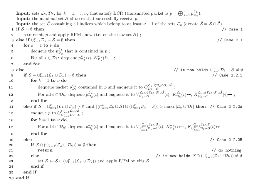
The following specific rules for packet movement (shown in pseudocode form in Fig. 2) have been devised according to the above rationale i.e. assuming, for now, that BP holds at the beginning of slot $t$ , we should move the packets in such a way that BP also holds at the end of slot $t$ . For the reader’s benefit, we provide a high level description of the algorithmic logic for each case and we use a mnemonic name in parentheses to easily distinguish the cases.

Rules for Packet Movement (RPM): Let packet $p$ of the form $p=\bigoplus_{k=1}^{\nu}p_{\mathcal{D}_{k}}^{\mathcal{L}_{k}}$ satisfying the Basic Coding Rule (BCR) be chosen for transmission at slot $t$ , and let $\mathcal{S}$ be the maximal set of users that receive $p$ (i.e. the packet is erased by all users in $\mathcal{S}^{c}$ ). We define the set $\tilde{\mathcal{L}}$ as follows: $i\in\tilde{\mathcal{L}}$ iff $i$ belongs to at least $\nu-1$ of the sets $\mathcal{L}_{k}$ , for $k=1,\ldots,\nu$ . Hence, before transmission of $p$ , user $i\in\tilde{\mathcal{L}}$ is a Listener for all but at most one of the packets $p_{\mathcal{D}_{k}}^{\mathcal{L}_{k}}$ , with $k=1,\ldots,\nu$ . We also denote with $\tilde{\mathcal{S}}=\mathcal{S}\cap\tilde{\mathcal{L}}$ the set of users in $\tilde{\mathcal{L}}$ that received $p$ . Note that it is quite possible for $\tilde{\mathcal{S}}$ to be empty even though $\mathcal{S}\neq\emptyset$ (e.g. $p=p_{2}^{1}\oplus p_{1}^{2}$ , which satisfies BCR, with $\mathcal{S}=\left\{3\right\}$ and $\tilde{\mathcal{L}}=\{1,2\}$ ). The following rules are now checked and the corresponding actions are performed (if applicable). Although only the real packets and queues are handled by the transmitter, we also consider (at a conceptual level) the virtual network and describe how it would be affected in each case.

1.

( $p$ is erased by all users): If $\mathcal{S}=\emptyset$ , then the transmitted packet is erased by all users. Hence, no new information is gained by the users and the Destination/Listener sets for each packet in the network remains unaffected (the current slot essentially being “wasted”), which implies that no packet movement occurs and $p$ is retransmitted in the next slot.
2.
Otherwise, it holds $\mathcal{S}\neq\emptyset$ . In this case, by Corollary 1 and Fact 1, all users in $\cup_{k=1}^{\nu}\mathcal{D}_{k}$ (i.e. the Destinations of packet $p$ ) that receive $p$ can instantly decode their unknown native packet, i.e. for all $k\in\left\{1,\ldots,\nu\right\}$ and $i\in\mathcal{D}_{k}\cap\mathcal{S}$ , packet $p_{\mathcal{D}_{k}}^{\mathcal{L}_{k}}(i)$ is decoded by $i$ and its corresponding token is removed from the virtual network (as a result, $K^{\mathcal{L}_{k}}_{\mathcal{D}_{k}}(i)$ is reduced by 1). Notice also that any $i\in\mathcal{D}_{k}\cap\mathcal{S}$ becomes a Listener for $p_{\mathcal{D}_{k}}^{\mathcal{L}_{k}}$ after receiving $p$ . Regarding the potential packet movements and counter changes:
1. 2.1)
  
  (all Destinations of $p$ receive $p$ ): If $\cup_{k=1}^{\nu}\mathcal{D}_{k}\subseteq\mathcal{S}$ (i.e. $\cup_{k=1}^{\nu}\mathcal{D}_{k}-\mathcal{S}=\emptyset$ ), then all native packets $p^{\mathcal{L}_{k}}_{\mathcal{D}_{k}}(i)$ , for $k=1,\ldots,\nu$ and $i\in\mathcal{D}_{k}$ , are instantly decoded by their intended destinations and their tokens are removed from the virtual network (as explained above), since the corresponding native packets are no longer useful, having been decoded by their intended users. For the same reason, for $k=1,\ldots,\nu$ , all packets $p^{\mathcal{L}_{k}}_{\mathcal{D}_{k}}$ that comprise $p$ are removed from the respective queue $Q^{\mathcal{L}_{k}}_{\mathcal{D}_{k}}$ and no other packet/token movement takes place.
2. 2.2)
  
  Otherwise, it holds $\cup_{k=1}^{\nu}\mathcal{D}_{k}-\mathcal{S}\neq\emptyset$ and we distinguish the following cases:
  1. 2.2.1)
    
    (only Destinations/Listeners of constituent packets of $p$ receive $p$ ): It holds $\mathcal{S}\subseteq\cup_{k=1}^{\nu}(\mathcal{L}_{k}\cup\mathcal{D}_{k})$ , equivalently $\hat{\mathcal{S}}=S-\cup_{k=1}^{\nu}(\mathcal{L}_{k}\cup\mathcal{D}_{k})=\emptyset$ . Notice that, for $\nu>1$ , the latter condition is equivalent, by the BCR, to $\mathcal{S}\subseteq\cup_{k=1}^{\nu}\mathcal{L}_{k}$ , while for $\nu=1$ it reduces to $\mathcal{S}\subseteq\mathcal{L}_{1}\cup\mathcal{D}_{1}$ . In both cases, and for each $k\in\left\{1,\ldots,\nu\right\}$ , packet $p_{\mathcal{D}_{k}}^{\mathcal{L}_{k}},\>\mathcal{{\rm where\>}D}_{k}-\mathcal{S}\neq\emptyset,$ is moved to queue $Q_{\mathcal{D}_{k}-\mathcal{S}}^{\mathcal{L}_{k}\cup\left(\mathcal{D}_{k}\cap\mathcal{S}\right)\cup\tilde{\mathcal{S}}}$ and, for each $i\in\mathcal{D}_{k}-\mathcal{S}$ , token $p^{\mathcal{L}_{k}}_{\mathcal{D}_{k}}(i)$ is moved to $V^{\mathcal{L}_{k}\cup(\mathcal{D}_{k}\cap\mathcal{S})\cup\tilde{\mathcal{S}}}_{\mathcal{D}_{k}-\mathcal{S}}(i)$ . Hence, counter $K^{\mathcal{L}_{k}}_{\mathcal{D}_{k}}(i)$ is reduced by 1 while $K^{\mathcal{L}_{k}\cup(\mathcal{D}_{k}\cap\mathcal{S})\cup\tilde{\mathcal{S}}}_{\mathcal{D}_{k}-\mathcal{S}}(i)$ is increased by 1. If, for some $k$ , it holds $\mathcal{D}_{k}-\mathcal{S}=\emptyset$ , then all $p_{\mathcal{D}_{k}}^{\mathcal{L}_{k}}$ are removed from the respective queues. The two cases $\mathcal{D}_{k}-\mathcal{S}\stackrel{{\scriptstyle\neq}}{{=}}\emptyset$ can be jointly handled following the convention that whenever a packet is moved to a queue $Q_{\mathcal{D}}^{\mathcal{L}}$ with $\mathcal{D}=\emptyset$ , it actually leaves the network. This will be systematically used below to avoid repetition. The consistency of these packet movements with Basic Properties is subsequently proved in Lemma 4. Hence, according to this rule, packet $p_{\mathcal{D}_{k}}^{\mathcal{L}_{k}}$ is either not moved at all (if $\tilde{\mathcal{S}}\cup\left(\mathcal{D}_{k}\cap\mathcal{S}\right)=\emptyset$ ), or is moved to a higher level (or within the same level but higher sublevel) queue, or exits the network completely (if $\mathcal{D}_{k}-\mathcal{S}=\emptyset$ ). Also notive that, as intuitively expected based on Definitions 1, 2, the current case guarantees that the Destination set (resp. Listenerr set) of a packet cannot decrease(resp. increase after a packet movement).
  2. 2.2.2)
    
    It holds $\hat{\mathcal{S}}=S-\cup_{k=1}^{\nu}(\mathcal{L}_{k}\cup\mathcal{D}_{k})\neq\emptyset$ / Again, this condition is equivalent to $\hat{\mathcal{S}}=\mathcal{S}-\cup_{k=1}^{\nu}\mathcal{L}_{k}\neq\emptyset$ , for $\nu>1$ , and $\hat{\mathcal{S}}=\mathcal{S}-(\mathcal{L}_{1}\cup\mathcal{D}_{1})\neq\emptyset$ for $\nu=1$ . We further distinguish two subcases:
    
    A.
    
    (received feedback creates a combined Listener/Destination set in a level higher than that of all constituent packets of $p$ ): If $\lvert\left(\cap_{k=1}^{\nu}\mathcal{L}_{k}\cup\mathcal{S}\right)\cup\left(\cup_{k=1}^{\nu}\mathcal{D}_{k}-\mathcal{S}\right)\rvert>\max_{k=1,\ldots,\nu}\lvert\mathcal{L}_{k}\cup\mathcal{D}_{k}\rvert$ ,²² 2 it is easy to verify that this inequality is always true for $\nu=1$ . then packet $p$ is moved to $Q_{\cup_{k=1}^{\nu}\mathcal{D}_{k}-\mathcal{S}}^{\cap_{k=1}^{\nu}\mathcal{L}_{k}\cup\mathcal{S}}$ and packets $p_{\mathcal{D}_{k}}^{\mathcal{L}_{k}}$ are removed from queues $Q_{\mathcal{D}_{k}}^{\mathcal{L}_{k}}$ . In the virtual network, for each $i\in\mathcal{D}_{k}-\mathcal{S}$ , token $p^{\mathcal{L}_{k}}_{\mathcal{D}_{k}}(i)$ is moved from $V^{\mathcal{L}_{k}}_{\mathcal{D}_{k}}(i)$ to $V^{\cap_{k=1}^{\nu}\mathcal{L}_{k}\cup\mathcal{S}}_{\cup_{k=1}^{\nu}\mathcal{D}_{k}-\mathcal{S}}(i)$ (so that counters $K^{\mathcal{L}_{k}}_{\mathcal{D}_{k}}(i)$ and $K_{\cup_{k=1}^{\nu}\mathcal{D}_{k}-\mathcal{S}}^{\cap_{k=1}^{\nu}\mathcal{L}_{k}\cup\mathcal{S}}\left(i\right)$ are reduced by 1 and increased by 1, respectively). Lemma 4 shows again that this packet movement is consistent with Basic Properties and the packets are moved only to higher level or sublevel queues (or exit the network).
    
    B.
    
    (no higher level Listener/Destination set, relative to constituent packets of $p$ , can be created based on received feedback): If $\lvert\left(\cap_{k=1}^{\nu}\mathcal{L}_{k}\cup\mathcal{S}\right)\cup\left(\cup_{k=1}^{\nu}\mathcal{D}_{k}-\mathcal{S}\right)\rvert\leq\max_{k=1,\ldots,\nu}\lvert\mathcal{L}_{k}\cup\mathcal{D}_{k}\rvert$ then
    
    •
    
    if $\mathcal{S}\cap\left(\cup_{k=1}^{\nu}(\mathcal{L}_{k}\cup\mathcal{D}_{k})\right)=\emptyset$ , no further action is taken.
    
    •
    
    else, set $\mathcal{S}\leftarrow\mathcal{S}\cap\left(\cup_{k=1}^{\nu}(\mathcal{L}_{k}\cup\mathcal{D}_{k})\right)$ and apply the above rules again for the new $\mathcal{S}$ . Notice that Case 2.2.1 is now applicable for the new $\mathcal{S}$ .

As previously mentioned, the validity of the above actions is proved in the following result, which in turn guarantees the instant decodability property. Induction on time then shows that BP is true for all slots $t$ if BCR and RPM are applied in each slot.

Lemma 4.

Assuming that the Basic Properties are satisfied at the beginning of slot $t$ , then the application of the Basic Coding Rule and Rules for Packet Movement to the packet transmitted at slot $t$ satisfies the Basic Properties at the beginning of slot $t+1$ .

Proof:

See Appendix -A. ∎Since the Rules for Packet Movement have a complicated logical structure, we provide the following concrete example for clarification.

Example 2.

Suppose packet $p=p_{1}^{2346}\oplus p_{24}^{135}\oplus p_{3}^{1246}$ is transmitted, so $\nu=3$ and $\mathcal{D}_{1}=\left\{1\right\},\mathcal{D}_{2}=\left\{2,4\right\},\mathcal{D}_{3}=\left\{3\right\},$ $\mathcal{L}_{1}=\left\{2,3,4,6\right\},$ $\mathcal{L}_{2}=\left\{1,3,5\right\},$ $\mathcal{L}_{3}=\left\{1,2,4,6\right\}$ . Hence, $\cup_{k=1}^{3}\mathcal{D}_{k}=\left\{1,2,3,4\right\}$ .

•

Suppose $p$ is received by users $2,5$ and $6$ , so $\mathcal{S}=\left\{2,5,6\right\}$ . It holds $\cup_{k=1}^{3}\mathcal{D}_{k}-\mathcal{S}=\left\{1,3,4\right\}\neq\emptyset$ and $\mathcal{\hat{\mathcal{S}}=S}-\cup_{k=1}^{3}(\mathcal{L}_{k}\cup\mathcal{D}_{k})=\left\{2,5,6\right\}-\left\{1,2,3,4,5,6\right\}=\emptyset$ , so we are in case 2.2.1. We have $\mathcal{S}\cap\left(\cup_{k=1}^{3}(\mathcal{L}_{k}\cup\mathcal{D}_{k})\right)=\mathcal{S}=\left\{2,5,6\right\}$ and $\tilde{\mathcal{S}}=\left\{2,6\right\}$ , because user $5$ does not belong to $\nu-1=2$ sets $\mathcal{L}_{k}$ but only to set $\mathcal{L}_{2}$ . The 3 packets are moved as follows:
- –
  
  packet $p_{1}^{2346}$ is not moved because $\mathcal{D}_{1}\cap\mathcal{S}=\left\{1\right\}\cap\left\{2,5,6\right\}=\emptyset$ (equivalently, it is moved to $Q_{\mathcal{D}_{1}-\mathcal{S}}^{\mathcal{L}_{1}\cup\left(\mathcal{D}_{1}\cap\mathcal{S}\right)\cup\tilde{\mathcal{S}}}$ , i.e. $Q_{\left\{1\right\}}^{\left\{2,3,4,6\right\}\cup\emptyset\cup\left\{2,6\right\}}=Q_{1}^{2346}$ , which is where it is currently stored).
- –
  
  packet $p_{24}^{135}$ is moved to $Q_{\mathcal{D}_{2}-\mathcal{S}}^{\mathcal{L}_{2}\cup\left(\mathcal{D}_{2}\cap\mathcal{S}\right)\cup\tilde{\mathcal{S}}}$ , i.e. $Q_{\left\{2,4\right\}-\left\{2,5,6\right\}}^{\left\{1,3,5\right\}\cup\left(\left\{2,4\right\}\cap\left\{2,5,6\right\}\right)\cup\left\{2,6\right\}}=Q_{4}^{12356}$ .
- –
  
  packet $p_{3}^{1246}$ is not moved because $\mathcal{D}_{3}\cap\mathcal{S}=\left\{3\right\}\cap\left\{2,5,6\right\}=\emptyset$ (equivalently, it is moved to $Q_{\mathcal{D}_{3}-\mathcal{S}}^{\mathcal{L}_{3}\cup\left(\mathcal{D}_{3}\cap\mathcal{S}\right)\cup\tilde{\mathcal{S}}}$ , i.e. $Q_{\left\{3\right\}}^{\left\{1,2,4,6\right\}\cup\emptyset\cup\left\{2,6\right\}}=Q_{3}^{1246}$ ).

•

Suppose now that $p$ is received by users $7$ and $8$ , so $\mathcal{S}=\left\{7,8\right\}$ . It holds $\cup_{k=1}^{3}\mathcal{D}_{k}-\mathcal{S}=\left\{1,2,3,4\right\}$ and $\mathcal{\hat{\mathcal{S}}=S}-\cup_{k=1}^{3}(\mathcal{L}_{k}\cup\mathcal{D}_{k})=\left\{7,8\right\}-\left\{1,2,3,4,5,6\right\}=\left\{7,8\right\}\neq\emptyset$ , so we are in case 2.2.2. We have

		$\displaystyle\left\|\left(\cap_{k=1}^{3}\mathcal{L}_{k}\cup\mathcal{S}\right)\cup\left(\cup_{k=1}^{3}\mathcal{D}_{k}-\mathcal{S}\right)\right\|$
		$\displaystyle=\left\|\left(\left(\left\{2,3,4,6\right\}\cap\left\{1,3,5\right\}\cap\left\{1,2,4,6\right\}\right)\cup\left\{7,8\right\}\right)\cup\left(\left(\left\{1\right\}\cup\left\{2,4\right\}\cup\left\{3\right\}\right)-\left\{7,8\right\}\right)\right\|$
		$\displaystyle=\left\|\left\{1,2,3,4,7,8\right\}\right\|=6.$

We also have

\max_{k=1,\ldots,3}\left|\mathcal{L}_{k}\cup\mathcal{D}_{k}\right|=\max\left\{\left|\left\{1,2,3,4,6\right\}\right|,\left|\left\{1,2,3,4,5\right\}\right|,\left|\left\{1,2,3,4,6\right\}\right|\right\}=5.

Therefore, we are in subcase 2.2.2A, and $p$ is moved to $Q_{\cup_{k=1}^{3}\mathcal{D}_{k}-\mathcal{S}}^{\cap_{k=1}^{3}\mathcal{L}_{k}\cup\mathcal{S}}$ , i.e. $Q_{1234}^{78}$ .

•

If $p$ is received by user $7$ , then $\mathcal{S}=\left\{7\right\}$ . It holds $\cup_{k=1}^{3}\mathcal{D}_{k}-\mathcal{S}\neq\emptyset$ and $\mathcal{\hat{\mathcal{S}}=S}-\cup_{k=1}^{3}(\mathcal{L}_{k}\cup\mathcal{D}_{k})=\left\{7\right\}-\left\{1,2,3,4,5,6\right\}=\left\{7\right\}\neq\emptyset$ , so we are in case 2.2.2. We have

\left|\left(\cap_{k=1}^{3}\mathcal{L}_{k}\cup\mathcal{S}\right)\cup\left(\cup_{k=1}^{3}\mathcal{D}_{k}-\mathcal{S}\right)\right|=\left|\left\{1,2,3,4,7\right\}\right|=5,

•

If $p$ is received by users $2$ and $7$ , then $\mathcal{S}=\left\{2,7\right\}$ . We have $\cup_{k=1}^{3}\mathcal{D}_{k}-\mathcal{S}\neq\emptyset$ and $\mathcal{\hat{\mathcal{S}}=S}-\cup_{k=1}^{3}(\mathcal{L}_{k}\cup\mathcal{D}_{k})=\left\{2,7\right\}-\left\{1,2,3,4,5,6\right\}=\left\{7\right\}\neq\emptyset$ , so we are in case 2.2.2. We have

\left|\left(\cap_{k=1}^{3}\mathcal{L}_{k}\cup\mathcal{S}\right)\cup\left(\cup_{k=1}^{3}\mathcal{D}_{k}-\mathcal{S}\right)\right|=\left|\left\{1,2,3,4,7\right\}\right|=5,

and $\max_{k=1,\ldots,3}\left|\mathcal{L}_{k}\cup\mathcal{D}_{k}\right|=5$ . We also have $\mathcal{S}\cap\left(\cup_{k=1}^{3}(\mathcal{L}_{k}\cup\mathcal{D}_{k})\right)=\left\{2,7\right\}\cap\left\{1,2,3,4,5,6\right\}=\left\{2\right\}\neq\emptyset$ , therefore we are in the second case of 2.2.2B. Next, we set $\mathcal{S}\leftarrow\mathcal{S}\cap\left(\cup_{k=1}^{3}(\mathcal{L}_{k}\cup\mathcal{D}_{k})\right)$ , i.e. $\mathcal{S}\leftarrow\left\{2\right\}$ , and apply the same rules to the new $\mathcal{S}$ , which brings us to case 2.2.1. We have $\tilde{\mathcal{S}}=\left\{2\right\}$ and the 3 packets are moved as follows:

–

packet $p_{1}^{2346}$ is not moved because $\mathcal{D}_{1}\cap\mathcal{S}=\left\{1\right\}\cap\left\{2\right\}=\emptyset$ (equivalently, it is moved to $Q_{\mathcal{D}_{1}-\mathcal{S}}^{\mathcal{L}_{1}\cup\left(\mathcal{D}_{1}\cap\mathcal{S}\right)\cup\tilde{\mathcal{S}}}$ , i.e. $Q_{\left\{1\right\}}^{\left\{2,3,4,6\right\}\cup\emptyset\cup\left\{2\right\}}=Q_{1}^{2346}$ ).
–

packet $p_{24}^{135}$ is moved to $Q_{\mathcal{D}_{2}-\mathcal{S}}^{\mathcal{L}_{2}\cup\left(\mathcal{D}_{2}\cap\mathcal{S}\right)\cup\tilde{\mathcal{S}}}$ , i.e. $Q_{\left\{2,4\right\}-\left\{2\right\}}^{\left\{1,3,5\right\}\cup\left(\left\{2,4\right\}\cap\left\{2\right\}\right)\cup\left\{2\right\}}=Q_{4}^{1235}$ .
–

packet $p_{3}^{1246}$ is not moved because $\mathcal{D}_{3}\cap\mathcal{S}=\left\{3\right\}\cap\left\{2\right\}=\emptyset$ (equivalently, it is moved to $Q_{\mathcal{D}_{3}-\mathcal{S}}^{\mathcal{L}_{3}\cup\left(\mathcal{D}_{3}\cap\mathcal{S}\right)\cup\tilde{\mathcal{S}}}$ , i.e. $Q_{\left\{3\right\}}^{\left\{1,2,4,6\right\}\cup\emptyset\cup\left\{2\right\}}=Q_{3}^{1246}$ ).

The above choice of the Rules for Packet Movement allows for potential feedback information loss, regarding which user knows which packet. This is best illustrated in the third case of Example 2 where, although user 7 becomes a Listener for packet $p$ at the end of slot $t$ , this information is actually discarded. As explained, this choice is made on intuitive grounds in order to keep the system manageable and amenable to analysis. However, as will be seen in the next Section, for $N=4$ even a more restrictive choice of rules suffices to implement a policy with asymptotically (as packet length increases) maximal stability region when the channel erasure probabilities are i.i.d.

III-D Comparison between the Rules for Packet Movement and the rules in [3]

The reader who is familiar with the work in [3] will notice that the current RPM constitute an involved extension and strict generalization of the rules in [3], i.e. all allowable packet movements in [3] are still allowable in this work (and additional movements, not possible in [3], are now allowed). A proof of this fact entails a straightforward enumeration of all possible feedback and application of the relevant RPM case and is omitted. However, for the reader’s benefit, we provide Tables I–VII, which summarize the packet movements for all phases in [3] and show which RPM case applies to them.

IV Stabilizing Scheduling Policy

In this Section, we investigate the design of policies that, under the coding restrictions and packet movements described in Section III, stabilize the system whenever possible. We first need some definitions.

TABLE I: Selecting

p_{i}

for transmission in phase 1 of XOR2 in [3].

user $i$	user $j$	user $k$	action performed in [3]	Corresponding case in RPM (for arbitrary $N$ )
user $i$	user $j$	user $k$	action performed in [3]	leading to identical action
R	R	R	dequeue $p_{i}$ ; user $i$ decodes	Case 2.1
R	R	E	dequeue $p_{i}$ ; user $i$ decodes	Case 2.1
R	E	R	dequeue $p_{i}$ ; user $i$ decodes	Case 2.1
R	E	E	dequeue $p_{i}$ ; user $i$ decodes	Case 2.1
E	R	R	dequeue $p_{i}$ , move $p_{i}$ to $Q^{jk}_{i}$	Case 2.2.2A
E	R	E	dequeue $p_{i}$ , move $p_{i}$ to $Q^{j}_{i}$	Case 2.2.2A
E	E	R	dequeue $p_{i}$ , move $p_{i}$ to $Q^{k}_{i}$	Case 2.2.2A
E	E	E	retransmit	Case 1

TABLE II: Selecting

p^{i}_{j}\oplus p^{j}_{i}

for transmission in phase 2 of XOR2 in [3].

user $i$	user $j$	user $k$	action performed in [3]	Corresponding case in RPM (for arbitrary $N$ )
user $i$	user $j$	user $k$	action performed in [3]	leading to identical action
R	R	R	dequeue $p_{i}^{j}$ , $p_{j}^{i}$ ; users $i,j$ decode	Case 2.1
R	R	E	dequeue $p_{i}^{j}$ , $p_{j}^{i}$ ; users $i,j$ decode	Case 2.1
R	E	R	dequeue $p_{i}^{j}$ , $p_{j}^{i}$ , move $p$ to $Q_{j}^{ik}$ ; user $i$ decodes	Case 2.2.2A
R	E	E	dequeue $p_{i}^{j}$ ; user $i$ decodes	Case 2.2.1
E	R	R	dequeue $p_{i}^{j}$ , $p_{j}^{i}$ , move $p$ to $Q_{i}^{jk}$ ; user $j$ decodes	Case 2.2.2A
E	R	E	dequeue $p_{j}^{i}$ ; user $j$ decodes	Case 2.2.1
E	E	R	dequeue $p_{i}^{j}$ , $p_{j}^{i}$ , move $p$ to $Q_{ij}^{k}$	Case 2.2.2A
E	E	E	retransmit	Case 1

TABLE III: Selecting

p^{i}_{jk}\oplus p^{jk}_{i}

for transmission in phase 3 (part 1) of XOR2 in [3].

user $i$	user $j$	user $k$	action performed in [3]	Corresponding case in RPM (for arbitrary $N$ )
user $i$	user $j$	user $k$	action performed in [3]	leading to identical action
R	R	R	dequeue $p_{i}^{jk},\>p_{jk}^{i}$ ; all 3 users decode	Case 2.1
R	R	E	dequeue $p_{i}^{jk},\>p_{jk}^{i}$ , move $p_{jk}^{i}$ to $Q_{k}^{ij}$ ; users $i,j$ decode	Case 2.2.1
R	E	R	dequeue $p_{i}^{jk},\>p_{jk}^{i}$ , move $p_{jk}^{i}$ to $Q_{j}^{ik}$ ; users $i,k$ decode	Case 2.2.1
R	E	E	dequeue $p_{i}^{jk}$ ; user $i$ decodes	Case 2.2.1
E	R	R	dequeue $p_{jk}^{i}$ ; users $j$ , $k$ decode	Case 2.2.1
E	R	E	dequeue $p_{jk}^{i}$ , move $p_{jk}^{i}$ to $Q_{k}^{ij}$ ; user $j$ decodes	Case 2.2.1
E	E	R	dequeue $p_{jk}^{i}$ , move $p_{jk}^{i}$ to $Q_{j}^{ik}$ ; user $k$ decodes	Case 2.2.1
E	E	E	retransmit	Case 1

TABLE IV: Selecting

p^{i}_{jk}

for transmission in phase 3 (part 2) of XOR2 in [3].

user $i$	user $j$	user $k$	action performed in [3]	Corresponding case in RPM (for arbitrary $N$ )
user $i$	user $j$	user $k$	action performed in [3]	leading to identical action
R	R	R	dequeue $p^{i}_{jk}$ ; users $j,k$ decode	Case 2.1
R	R	E	dequeue $p^{i}_{jk}$ ; move $p^{i}_{jk}$ to $Q^{ij}_{k}$ ; user $j$ decodes	Case 2.2.1
R	E	R	dequeue $p^{i}_{jk}$ , move $p^{i}_{jk}$ to $Q^{ik}_{j}$ ; user $k$ decodes	Case 2.2.1
R	E	E	$p^{i}_{jk}$ remains in $Q^{i}_{jk}$	Case 2.2.1
E	R	R	dequeue $p^{i}_{jk}$ ; users $j,k$ decode	Case 2.1
E	R	E	dequeue $p^{i}_{jk}$ , move $p^{i}_{jk}$ to $Q^{ij}_{k}$ ; user $j$ decodes	Case 2.2.1
E	E	R	dequeue $p^{i}_{jk}$ , move $p^{i}_{jk}$ to $Q^{ik}_{j}$ ; user $k$ decodes	Case 2.2.1
E	E	E	retransmit	Case 1

TABLE V: Selecting

p^{j}_{i}\oplus p^{ik}_{j}

for transmission in phase 4 (part 1) of XOR2 in [3].

user $i$	user $j$	user $k$	action performed in [3]	Corresponding case in RPM (for arbitrary $N$ )
user $i$	user $j$	user $k$	action performed in [3]	leading to identical action
R	R	R	dequeue $p^{j}_{i}$ , $p^{ik}_{j}$ ; users $i,j$ decode	Case 2.1
R	R	E	dequeue $p^{j}_{i}$ , $p^{ik}_{j}$ ; users $i,j$ decode	Case 2.1
R	E	R	dequeue $p^{j}_{i}$ ; user $i$ decodes	Case 2.2.1
R	E	E	dequeue $p^{j}_{i}$ ; user $i$ decodes	Case 2.2.1
E	R	R	dequeue $p^{j}_{i}$ , $p^{ik}_{j}$ , move $p^{j}_{i}$ to $Q^{jk}_{i}$ ; user $j$ decodes	Case 2.2.1
E	R	E	dequeue $p^{ik}_{j}$ ; user $j$ decodes	Case 2.2.1
E	E	R	dequeue $p^{j}_{i}$ , move $p^{j}_{i}$ to $Q^{jk}_{i}$	Case 2.2.1
E	E	E	retransmit	Case 1

TABLE VI: Selecting

p^{j}_{i}

for transmission in phase 4 (part 2) of XOR2 in [3].

user $i$	user $j$	user $k$	action performed in [3]	Corresponding case in RPM (for arbitrary $N$ )
user $i$	user $j$	user $k$	action performed in [3]	leading to identical action
R	R	R	dequeue $p^{j}_{i}$ ; user $i$ decodes	Case 2.1
R	R	E	dequeue $p^{j}_{i}$ ; user $i$ decodes	Case 2.1
R	E	R	dequeue $p^{j}_{i}$ ; user $i$ decodes	Case 2.1
R	E	E	dequeue $p^{j}_{i}$ ; user $i$ decodes	Case 2.1
E	R	R	dequeue $p^{j}_{i}$ , move $p^{j}_{i}$ to $Q^{jk}_{i}$	Case 2.2.2A
E	R	E	$p^{j}_{i}$ remains in $Q^{j}_{i}$	Case 2.2.1
E	E	R	dequeue $p^{j}_{i}$ , move $p^{j}_{i}$ to $Q^{jk}_{i}$	Case 2.2.2A
E	E	E	retransmit	Case 1

IV-A System Stability and Stability Region

Let $X\left(t\right),$ $t=0,1,\ldots$ be a stochastic process.

Definition 3 (Stability).

The process $X\left(t\right),$ $t=0,1,\ldots$ is stable iff

\lim_{q\rightarrow\infty}\underset{{\scriptstyle t\rightarrow\infty}}{\limsup}\Pr\left(X\left(t\right)>q\right)=0.

TABLE VII: Selecting

p^{jk}_{i}\oplus p^{ik}_{j}\oplus p^{ij}_{k}

for transmission in phase 5 of XOR2 in [3].

user $i$	user $j$	user $k$	action performed in [3]	Corresponding case in RPM (for arbitrary $N$ )
user $i$	user $j$	user $k$	action performed in [3]	leading to identical action
R	R	R	dequeue $p^{jk}_{i}$ , $p^{ik}_{j}$ , $p^{ij}_{k}$ ; users $i,j,k$ decode	Case 2.1
R	R	E	dequeue $p^{jk}_{i}$ , $p^{ik}_{j}$ ; users $i,j$ decode	Case 2.2.1
R	E	R	dequeue $p^{jk}_{i}$ , $p^{ij}_{k}$ ; users $i,k$ decode	Case 2.2.1
R	E	E	dequeue $p^{jk}_{i}$ ; user $i$ decodes	Case 2.2.1
E	R	R	dequeue $p^{ik}_{j}$ , $p^{ij}_{k}$ ; users $j,k$ decode	Case 2.2.1
E	R	E	dequeue $p^{ik}_{j}$ ; user $j$ decodes	Case 2.2.1
E	E	R	dequeue $p^{ij}_{k}$ ; user $k$ decodes	Case 2.2.1
E	E	E	retransmit	Case 1

Consider next a time-slotted system $\mathcal{U}$ . At the beginning of each slot, a number of new packets belonging to a set $\mathcal{N}$ of “flows” arrive to the system. Newly arriving packets of flow $i\in\mathcal{N}$ are placed at infinite size queues, i.e. no incoming packets are ever dropped. These packets are processed by a policy $\pi$ belonging to a set $\Pi$ of admissible policies. We hereafter use the term “policy” to refer to a collection of rules for choosing which packets, stored in a set of queues $\mathcal{Q}$ , to combine through a XOR operation and how to move packets between the queues in $\mathcal{Q}$ (the rules also allow for a packet to exit the system). The exact rules will be stated later. Let $A_{i}\left(t\right)$ , $i\in\mathcal{N}$ , be the number of flow $i$ packets arriving at the system at the beginning of slot $t.$ For the purposes of this paper, we assume that the process $\left\{\boldsymbol{A}(t)\right\}_{t=0}^{\infty}$ , where $\boldsymbol{A}\left(t\right)=\left(A_{i}(t):\,i\in\mathcal{N}\right)$ , consists of i.i.d vectors with $\mathbb{E}[\boldsymbol{A}(t)]=\boldsymbol{\lambda}\geq\boldsymbol{0}$ . We denote with $Q_{l}^{\pi}\left(t\right)$ the number of packets in queue $Q_{l}\in\mathcal{Q}$ at time $t$ when policy $\pi\in\Pi$ is applied, and define $\hat{Q}^{\pi}(t)=\sum_{Q_{l}\in\mathcal{Q}}Q_{l}^{\pi}\left(t\right).$

Definition 4 (System Stability).

1.

For a given arrival rate vector $\boldsymbol{\lambda}$ , system $\mathcal{U}$ is stable under policy $\pi$ if the process $\hat{Q}^{\pi}(t)$ is stable.
2.

The stability region $\mathcal{R}^{\pi}$ of a policy $\pi\in\Pi$ is the closure of the set of arrival rates for which $\mathcal{U}$ is stable under $\pi$ .
3.

The stability region $\mathcal{R}_{\Pi}$ of system $\mathcal{U}$ under the set of policies $\Pi$ is the closure of the set $\cup_{\pi\in\Pi}\mathcal{R}^{\pi}.$
4.

A policy $\pi^{*}\in\Pi$ is stabilizing within $\Pi$ if $\mathcal{R}_{\Pi}=\mathcal{R}^{\pi^{*}}$ .

Consider now the system under study in the current work. At the beginning of each slot, a decision must be made at the base station concerning the combination of packets from the real queues that must be XORed to form the packet $p=p_{\mathcal{D}_{1}}^{\mathcal{L}_{1}}\oplus\ldots\oplus p_{\mathcal{D}_{\nu}}^{\mathcal{L}_{\nu}}$ to be transmitted. Such a decision is called a “control” $I_{\mathcal{D}_{1},\ldots,\mathcal{D}_{\nu}}^{\mathcal{L}_{1},\ldots,\mathcal{L}_{\nu}}$ and we denote the set of such controls by $\mathcal{I}$ . Notice that, by definition, a control is identified by the set $\left\{\left(\mathcal{D}_{i},\mathcal{L}_{i}\right)\right\}_{i=1}^{\nu}$ and not by the order of the elements in the set, i.e. control $I_{\mathcal{D}_{1},\ldots,\mathcal{D}_{\nu}}^{\mathcal{L}_{1},\ldots,\mathcal{L}_{\nu}}$ is identical to control $I_{\mathcal{D}_{\sigma(1)},\ldots,\mathcal{D}_{\sigma(\nu)}}^{\mathcal{L}_{\sigma(1)},\ldots,\mathcal{L}_{\sigma(\nu)}}$ for any permutation $\sigma(i)$ of the indices on $\left\{1,\ldots,\nu\right\}$ .

We assume henceforth that the Basic Coding Rule is followed for the formation of packet $p$ . For this system, an admissible policy consists of selecting, at the beginning of each time slot, one of the available controls $I_{\mathcal{D}_{1},\ldots,\mathcal{D}_{\nu}}^{\mathcal{L}_{1},\ldots,\mathcal{L}_{\nu}}$ to form a packet $p$ for transmission. After $p$ is transmitted, packets are moved among the real queues $Q_{\mathcal{D}_{k}}^{\mathcal{L}_{k}}(i)$ according to the Rules for Packet Movement (RPM) described in Section III. We also consider the virtual network, where a token for an exogenous native packet for user $i\in\mathcal{N}$ is initially stored in $V_{i}(i)$ and then travels through the virtual network according to the RPM (as it now applies to the virtual queues only). Hence, there exist two different queue networks, a “real network” $\mathcal{Q}=\bigcup_{\mathcal{L},\mathcal{D}}\left\{Q^{\mathcal{L}}_{\mathcal{D}}\right\}$ and a “virtual network” $\mathcal{V}=\bigcup_{\mathcal{L},\mathcal{D}}\bigcup_{i\in\mathcal{D}}\left\{V^{\mathcal{L}}_{\mathcal{D}}(i)\right\}$ , although only the former is actually present in the transmitter (the latter should be understood as part of a thought experiment that facilitates the analysis).

We now identify $\Pi$ as the set of admissible policies that select transmitted packets according to the Basic Coding Rule and then move packets based on the Rules for Packet Movement. A characteristic of such movements is that the destination (i.e. queue) of a packet movement cannot be determined at the beginning of transmission since it depends on the feedback received after packet transmission. For example, assume that $N=3$ and control $I_{12,3}^{3,12}$ is applied, i.e. packet $p=p_{12}^{3}\oplus p_{3}^{12}$ is transmitted. The tokens involved in this transmission are $p_{12}^{3}(1),p_{12}^{3}(2),p_{3}^{12}(3)$ . Figure 3 shows the possible movements of these tokens according to the received feedback.

Under the above definition of $\Pi$ , any policy $\pi\in\Pi$ can be individually applied to the “real” and “virtual” network. Defining $\hat{Q}^{\pi}(t)=\sum_{\mathcal{L},\mathcal{D}}\lvert\left(Q^{\mathcal{L}}_{\mathcal{D}}(t)\right)^{\pi}\rvert$ and $\hat{V}^{\pi}(t)=\sum_{\mathcal{L},\mathcal{D}}\sum_{i\in\mathcal{D}}\lvert\left(V^{\mathcal{L}}_{\mathcal{D}}(i)(t)\right)^{\pi}\rvert$ as the total backlog at slot $t$ in each network (and hereafter dropping the $\pi$ superscript in the queues), we can use Lemma 1 to write

\hat{Q}^{\pi}(t)=\sum_{\mathcal{L},\mathcal{D}}\lvert Q^{\mathcal{L}}_{\mathcal{D}}(t)\rvert\leq\sum_{\mathcal{L},\mathcal{D}}\lvert\mathcal{D}\rvert\lvert Q^{\mathcal{L}}_{\mathcal{D}}(t)\rvert=\hat{V}^{\pi}(t)\leq\sum_{\mathcal{L},\mathcal{D}}N\lvert Q^{\mathcal{L}}_{\mathcal{D}}(t)\rvert,

(2)

since $\lvert\mathcal{D}\rvert\leq N$ , whence we conclude that $\frac{\hat{V}^{\pi}(t)}{N}\leq\hat{Q}^{\pi}(t)\leq\hat{V}^{\pi}(t)$ . The last inequality implies that the real and virtual networks have the same stability region. Surprisingly, it also implies that the total number of packets stored in the real queues at any time is generally less than the total number of unknown native packets at that time.

Furthermore, it turns out that the virtual network falls in the class of systems whose stability has been studied in [8]. We next summarize the formulation and main results in [8] in a manner that will be useful in the development that follows. Consider a slotted-time network with a node set $\mathcal{M}\cup\left\{d\right\}$ , where $d\not\in\mathcal{M}$ , and directed edge (i.e. link) set ${\cal E}$ , where the special node $d$ represents the destination of traffic originated at the nodes in $\mathcal{M}$ (for now, assume there is a single destination for all traffic). Let $\mathcal{E}_{out}^{m},\>\mathcal{E}_{in}^{m}$ denote, respectively, the set of outgoing links and incoming links to node $m\in\mathcal{M}$ and assume that $\mathcal{E}_{out}^{m}\neq\emptyset$ for all $m\in\mathcal{M}$ . We allow self-loops in the network, i.e. for node $m\in\mathcal{M}$ , there may be a link $(m,m),$ implying that the sets $\mathcal{E}_{out}^{m},\>\mathcal{E}_{in}^{m}$ may both contain node $m.$ A finite set of controls $\mathcal{I}$ is available. For each control $I\in\mathcal{I},$ “transmission” takes place over the set of outgoing links $\mathcal{E}_{out}^{m}$ of node $m\in\mathcal{M}$ in a random manner as follows.

•

If, at a given slot, control $I\in\mathcal{I}$ is applied, then, for any node $m\in\mathcal{M}$ , at most $\hat{\mu}_{m}(I)\in\left\{0,1\right\}$ packets may be transmitted “over the set” $\mathcal{E}_{out}^{m}$ in the following random manner: For each $I\in\mathcal{I}$ , there is a random sequence $R_{n}^{m}(I)$ , with $n\geq 1$ , $m\in\mathcal{M}$ , where each $R_{n}^{m}\left(I\right)$ takes values in the set $\mathcal{E}_{out}^{m},$ with the following interpretation. A packet (if any) transmitted from node $m$ over the set $\mathcal{E}_{out}^{m}$ when control $I$ is applied for the $n$ -th time, is received only by the recipient of the link $R_{n}^{m}\left(I\right).$ Of course, if $R_{n}^{m}\left(I\right)=(m,m)$ then the packet is not received by any node in $\mathcal{E}_{out}^{m}$ - $\left\{m\right\},$ hence it remains at node $m$ .

For a given $n$ and $I$ , the random variables $R_{n}^{m}\left(I\right),\ m\in\mathcal{M},$ may be arbitrarily correlated. Moreover, we assume that for each control $I\in\mathcal{I},$ the random sequences $\left\{R_{n}^{m}\left(I\right),\ m\in\mathcal{M}\right\}_{n=1}^{\infty}$ are i.i.d., independent of the arrival processes, and define $p_{e}^{m}\left(I\right)\triangleq\Pr\left(R_{n}^{m}\left(I\right)=e\right)$ for $e\in\mathcal{E}_{out}^{m}$ so that

\sum_{e\in\mathcal{E}_{out}^{m}}p_{e}^{m}(I)=1\quad\forall\,m\in\mathcal{M},\,\forall\,I\in\mathcal{I}.

(3)

Strictly speaking, the description above is for nodes for which $\hat{\mu}_{m}\left(I\right)>0.$ In case $\hat{\mu}_{m}\left(I\right)=0$ for some $m\in\mathcal{M}$ , to avoid complicated notation, it is helpful to set $R_{n}^{m}\left(I\right)=e_{0}$ for some fixed $e_{0}\in\mathcal{E}_{out}^{m}$ .

To describe the stability region $\mathcal{R}_{\Pi}$ of this network, we need some preliminary definitions. For control $I\in\mathcal{I}$ , we define the set $\Gamma(I)$ of vectors $\boldsymbol{f}$ as

\Gamma\left(I\right)=\left\{\boldsymbol{f}=(f_{e})_{e\in\mathcal{E}}:\>f_{e}=p_{e}^{m}(I)\mu_{m},\>0\leq\mu_{m}\leq\hat{\mu}_{m}(I),\;m\in\mathcal{M},\,e\in\mathcal{E}_{out}^{m}\right\},

(4)

and the convex hull $\mathcal{H}$ of the sets $\Gamma(I)$ as

\mathcal{H}=\mathrm{conv}\left(\Gamma\left(I\right),I\in\mathcal{I}\right).

(5)

The stability region of the network $(\mathcal{M}\cup\{d\},\mathcal{E})$ is described by the following Theorem.

Theorem 1.

[8] The stability region $\mathcal{R}_{\Pi}$ of the system is the set of arrival rates $\boldsymbol{\lambda}=\left\{\lambda_{m}\right\}_{m\in\mathcal{M}}$ , $\lambda_{m}\geq 0$ , for which there exists a vector $\boldsymbol{f}\in\mathcal{H}$ such that for all nodes $m\in\mathcal{M}$ it holds

\sum_{e\in\mathcal{E}_{in}^{m}}f_{e}+\lambda_{m}\leq\sum_{e\in\mathcal{E}_{out}^{m}}f_{e}.

(6)

We will apply the formulation described above to the network consisting of the virtual queues $V_{\mathcal{D}}^{\mathcal{L}}(i),\>i\in\mathcal{D},$ i.e., we consider $\mathcal{M}=\left\{V_{\mathcal{D}}^{\mathcal{L}}(i):\>i\in\mathcal{D}\right\}$ for all $\mathcal{L},\mathcal{D}$ that satisfy CC. For this network, since at most one virtual packet (i.e. token) is transmitted per slot from any queue $m$ , we have $\hat{\mu}_{m}(I)\in\left\{0,1\right\}$ , $m\in\mathcal{M}$ . Also, the packet transition probabilities $p_{e}^{m}\left(I\right)$ for nodes with $\hat{\mu}_{m}(I)=1$ can be easily calculated (an example is given below). The only difference between the network $(\mathcal{M}\cup\left\{d\right\},\mathcal{E})$ and our model is that, in the latter, there are $N$ token destinations, $d_{i},\>i\in\mathcal{N}$ (one for each of the receivers) instead of a single one. However, we can combine all these destinations to a single destination $d$ , so that any token arriving in $d_{i}$ is considered to arrive at $d$ . This affects neither the admissible policies, nor the queue sizes at the various native queues at the base station. Hence, system stability is not affected, provided that we are interested in the total queue size at the base station.

Example 3.

Consider the case $N=3$ and assume that control $I_{12,3}^{3,12}$ is chosen, hence a combination $p=p_{12}^{3}\oplus p_{3}^{12}$ is transmitted, where $p_{12}^{3}=p_{12}^{3}\left(1\right)\oplus p_{12}^{3}\left(2\right)$ and $p_{3}^{12}=p_{3}^{12}\left(3\right)$ (recall Section III-A for the interpretation of the parentheses). The transition probabilities are then as follows:

•

Token $p_{12}^{3}\left(1\right)$ :
1. 1.
  
  If $p$ is received by user $1$ , $p_{12}^{3}\left(1\right)$ is removed from $V_{12}^{3}\left(1\right)$ and delivered to $d_{1}$ (i.e. to $d$ for the equivalent network). This event has probability $P_{\emptyset,\left\{1\right\}}$ .
2. 2.
  
  If $p$ is erased at user 1 and received by user 2, packet $p_{12}^{3}$ is moved to queue $Q_{1}^{23}$ and token $p_{12}^{3}\left(1\right)$ is moved to $V_{1}^{23}\left(1\right)$ . This event has probability $P_{\left\{1\right\},\left\{2\right\}}$ .
3. 3.
  
  If $p$ is erased at users 1 and 2, $p_{12}^{3}\left(1\right)$ remains at $V_{12}^{3}\left(1\right)$ . This event has probability $P_{\left\{1,2\right\},\emptyset}$ .
•

Token $p_{12}^{3}\left(2\right)$ : the transition probabilities are determined as in the previous case, by interchanging the indices 1, 2.
•
Token $p_{3}^{12}\left(3\right)$ :
1. 1.
  
  If $p$ is received by user 3, $p_{3}^{12}\left(3\right)$ is removed from $V_{3}^{12}\left(3\right)$ and delivered to $d_{3}$ . This event has probability $P_{\emptyset,\left\{3\right\}}$ .
2. 2.
  
  If $p$ is erased at $3,$ $p_{3}^{12}\left(3\right)$ remains at $V_{3}^{12}\left(3\right)$ . This event has probability $P_{\left\{3\right\},\emptyset}$ .

We now describe the stability region of Theorem 1 in a form that is more convenient for calculations. Any $\boldsymbol{f}$ in $\mathcal{H}$ can be written in the form

\boldsymbol{f}=\sum_{I\in\mathcal{I}}\phi_{I}\boldsymbol{f}\left(I\right),\mbox{ for some }\left\{\phi_{I}\right\}_{I\in\mathcal{I}}\mbox{ such that }\phi_{I}\geq 0,\>\sum_{I\in\mathcal{I}}\phi_{I}\leq 1,

(7)

where

\boldsymbol{f}\left(I\right)=\left(f_{e}\left(I\right)\right)_{e\in\mathcal{E}},

f_{e}\left(I\right)=p_{e}^{m}(I)\mu_{m}(I),\>0\leq\mu_{m}\left(I\right)\leq\hat{\mu}_{m}(I),\>m\in\mathcal{M},\,e\in\mathcal{E}_{out}^{m},

and, for any control $I=I_{\mathcal{D}_{1},\ldots,\mathcal{D}_{\nu}}^{\mathcal{L}_{1},\ldots,\mathcal{L}_{\nu}}$ , we define the set $\mathcal{M}(I)=\bigcup_{r=1}^{\nu}\bigcup_{k\in\mathcal{D}_{r}}\left\{V_{\mathcal{D}_{r}}^{\mathcal{L}_{r}}(k)\right\}$ so that

\hat{\mu}_{m}(I)=\left\{\begin{array}[]{cc}1&\text{if $m\in\mathcal{M}\left(I\right),$}\\ 0&\mbox{otherwise}.\end{array}\right.

(8)

In words, $\hat{\mu}_{m}(I)$ indicates whether control $I$ involves the queue corresponding to node $m$ for creation of the transmitted packet according to BCR.

Hence it holds,

\sum_{e\in\mathcal{E}_{out}^{m}}f_{e}=\sum_{e\in\mathcal{E}_{out}^{m}}\sum_{I\in\mathcal{I}}\phi_{I}f_{e}\left(I\right)=\sum_{I\in\mathcal{I}}\phi_{I}\sum_{e\in\mathcal{E}_{out}^{m}}p_{e}^{m}(I)\mu_{m}\left(I\right),

(9)

and

\sum_{e\in\mathcal{E}_{in}^{m}}f_{e}=\sum_{e\in\mathcal{E}_{in}^{m}}\sum_{I\in\mathcal{I}}\phi_{I}f_{e}\left(I\right)=\sum_{I\in\mathcal{I}}\sum_{e=(l,m)\in\mathcal{E}_{in}^{m}}\phi_{I}\mu_{l}\left(I\right)p_{e}^{l}(I).

(10)

Since the tokens for new packet arrivals are always placed in queues $V_{i}(i)$ , $i\in\mathcal{N}$ , we define

\bar{\lambda}_{m}=\begin{cases}1&\mbox{if }m=V_{i}(i),\\ 0&\mbox{otherwise}.\end{cases}

(11)

Replacing (9), (10) in (6), we have

\sum_{I\in\mathcal{I}}\phi_{I}\left(\sum_{e=(l,m)\in\mathcal{E}_{in}^{m}}\mu_{l}\left(I\right)p_{e}^{l}(I)\right)+\bar{\lambda}_{m}\leq\sum_{I\in\mathcal{I}}\phi_{I}\left(\sum_{e\in\mathcal{E}_{out}^{m}}p_{e}^{m}(I)\mu_{m}\left(I\right)\right),\quad m\in\mathcal{M},

(12)

or equivalently, taking into account (3),

\displaystyle\sum_{I\in\mathcal{I}}\phi_{I}\left(\sum_{\begin{subarray}{c}e=(l,m)\in\mathcal{E}_{in}^{m}\\ l\neq m\end{subarray}}\mu_{l}\left(I\right)p_{e}^{l}(I)\right)+\bar{\lambda}_{m}

\displaystyle\leq\sum_{I\in\mathcal{I}}\left(1-p_{(m,m)}^{m}(I)\right)\mu_{m}\left(I\right)\phi_{I},\quad m\in\mathcal{M},

(13)

Hence, the stability region $\mathcal{R}_{\Pi}$ of the system is described by either one of (12), (13), combined with

$\displaystyle 0\leq\mu_{m}\left(I\right)$	$\displaystyle\leq\hat{\mu}_{m}(I),$	(14)
$\displaystyle\phi_{I}$	$\displaystyle\geq 0,$	(15)
$\displaystyle\sum_{I\in\mathcal{I}}\phi_{I}$	$\displaystyle\leq 1,$	(16)

where $\hat{\mu}_{m}\left(I\right)$ is given by (8).

Two implementation issues are worth mentioning at this point. First, there must exist a mechanism for the receivers to know the constituents of the XOR combination of each received packet, in order to be able to use this packet in the decoding process. The simplest way to implement this is to use packet addresses to identify the native packets involved in the XOR combination of the transmitted packet. These addresses can be placed in the packet header. Reserving bits to describe packet addresses implies some loss of throughput due to the introduced overhead. To simplify the description, in the current and next Section we do not take the overhead into account and address the issue of stability in packets per slot. In Section VII, we discuss the number of addressed needed and loss of throughput due to overhead.

The second issue is that, under the schemes described in Section III, the receivers need to save received packets so that they can correctly decode at a later time. The stability results above consider only the queues at the base station. Hence, if we are interested in taking the receiver queues into consideration as well, we must ensure that the system remains stable even if the sizes of these queues are added to the total queue size at the base station. In fact, if the receivers are never informed by the base station as to which of their received packets will not be needed in the future, it is easy to devise scenarios where the queue sizes at the receivers grow to infinity even though the queues at the base station are stable. A simple way to deal with this problem is described in Section VII.

IV-B Stabilizing Policy

Applying directly the results in [8], we obtain the stabilizing policy described below. At the beginning of each time slot, the policy chooses a control of the form $I=I_{\mathcal{D}_{1},\ldots,\mathcal{D}_{\nu}}^{\mathcal{L}_{1},\ldots,\mathcal{L}_{\nu}}\in\mathcal{I}$ , where all counters $K^{\mathcal{L}_{r}}_{\mathcal{D}_{r}}(k)$ , for $r=1,\ldots,\nu$ and $k\in\mathcal{D}_{r}$ , are non-zero³³ 3 recall that $K^{\mathcal{L}_{r}}_{\mathcal{D}_{r}}(k)$ is defined as the number of tokens in virtual queue $V^{\mathcal{L}_{r}}_{\mathcal{D}_{r}}(k)$ and, by Lemma 1, can be deduced by information available in the real network. Hence, $K^{\mathcal{L}_{r}}_{\mathcal{D}_{r}}(k)>0$ is equivalent to saying that $V^{\mathcal{L}_{r}}_{\mathcal{D}_{r}}(k)$ is non-empty. and forms the appropriate packet to be transmitted in that slot, $p=\oplus_{r=1}^{\nu}p_{\mathcal{D}_{r}}^{\mathcal{L}_{r}}$ , according to the Basic Coding Rule. If control $I$ is chosen, one token from each of the queues in the set $\mathcal{M}\left(I\right)=\bigcup_{r=1}^{\nu}\bigcup_{k\in\mathcal{D}_{r}}\left\{V^{\mathcal{L}_{r}}_{\mathcal{D}_{r}}(k)\right\}$ may be moved to another virtual queue inside the network, or may reach the destination (thus, the native packet corresponding to the token exits the network). No packets from any of the other queues are moved. The algorithm for choosing the appropriate control is the following.

Algorithm 1: At each decision slot:

For each control $I=I_{\mathcal{D}_{1},\ldots,\mathcal{D}_{\nu}}^{\mathcal{L}_{1},\ldots,\mathcal{L}_{\nu}}\in\mathcal{I}$ that satisfies the BCR:

•

Form the weights

c_{m}\left(I\right)=\max\left\{K_{m}-\underset{{\scriptstyle e=(m,l)\in\mathcal{E}_{out}^{m}}}{\sum}p_{e}^{m}\left(I\right)K_{l},\>0\right\},\;m\in\mathcal{M}\left(I\right),

where $K_{m}$ is the length of the queue corresponding to node $m$ (corresponding to a queue in the virtual network, i.e. if $m=V^{\mathcal{L}}_{\mathcal{D}}(i)$ for some $\mathcal{L},\mathcal{D}$ and $i\in\mathcal{D}$ , then $K_{m}=K^{\mathcal{L}}_{\mathcal{D}}(i)$ ).

•

Form the reward under the given control,

$C\left(I\right)=\underset{m\in\mathcal{M}\left(I\right)}{\sum}c_{m}\left(I\right).$

2.

Find the control that maximizes the reward, i.e. $I^{\ast}=\arg\max{}_{I\in\mathcal{I}}C\left(I\right)$ , transmit the packet $p=\bigoplus_{k=1}^{\nu^{\ast}}p^{\mathcal{L}^{\ast}_{k}}_{\mathcal{D}^{\ast}_{k}}$ that corresponds to control $I^{\ast}=I^{\mathcal{L}^{\ast}_{1},\ldots,\mathcal{L}^{\ast}_{\nu^{\ast}}}_{\mathcal{D}^{\ast}_{1},\ldots,\mathcal{D}^{\ast}_{\nu^{\ast}}}$ and apply the Rules for Packet Movement after reception of feedback (including updating the $K$ counters).

Example 4.

Consider a network of $N=2$ users. The virtual queue network can be seen in Figure 4, where $d_{1}$ and $d_{2}$ are the two destination nodes. The set of all controls that obey the BCR is $\mathcal{I}=\left\{I_{1},I_{2},I_{1}^{2},I_{2}^{1},I_{1,2}^{2,1}\right\}$ . Suppose all queues are non empty. At each decision slot:

1.

For each control $I\in\mathcal{I}$ :
- •
  
  The set $\mathcal{M}\left(I\right)$ is formed. Table VIII shows the set $\mathcal{M}(I)$ for each control.
- •
  
  The next step is forming the weights $c_{m}\left(I\right)$ for every $I$ . For every node $m\in\mathcal{M}\left(I\right)$ , all possible outgoing edges $e=(m,l)$ in set $\mathcal{E}_{out}^{m}$ , when applying control $I$ , or equivalently, all receiving nodes $l$ , must be determined. Table IX shows all receiving nodes for each node $m$ , as well as the respective transition probabilities.
- •
  
  Next, for each node $m\in\mathcal{M}(I)$ and each control $I$ the weight $c_{m}\left(I\right)$ is calculated, as can be seen in Table X.
- •
  
  Then, for each control $I$ the reward $C\left(I\right)$ is determined (Table XI).

Finally, select the control that maximizes the reward

I^{*}=\arg\max{}_{I\in\mathcal{I}}C\left(I\right)=\arg\max\left\{C\left(I_{1}\right),C\left(I_{2}\right),C\left(I_{1}^{2}\right),C\left(I_{2}^{1}\right),C\left(I_{1,2}^{2,1}\right)\right\}.

The previous example is simple enough that the stability region of the proposed algorithm can be analytically determined as follows. For arrival rates $\lambda_{1},\lambda_{2}$ , we use the transition probabilities in Table IX and apply (12), (14)–(16) to get the following set of inequalities (recall the notational shortcut at the end of Section II)

$\displaystyle V_{1}(1):\lambda_{1}$	$\displaystyle\leq(1-\epsilon_{12})\phi_{1},$	(17)
$\displaystyle V_{2}(2):\lambda_{2}$	$\displaystyle\leq(1-\epsilon_{12})\phi_{2},$	(18)
$\displaystyle V^{2}_{1}(1):(\epsilon_{1}-\epsilon_{12})\phi_{1}$	$\displaystyle\leq(1-\epsilon_{1})\left(\phi^{2}_{1}+\phi^{2,1}_{1,2}\right),$	(19)
$\displaystyle V^{1}_{2}(2):(\epsilon_{2}-\epsilon_{12})\phi_{2}$	$\displaystyle\leq(1-\epsilon_{2})\left(\phi^{1}_{2}+\phi^{2,1}_{1,2}\right),$	(20)

with the additional constraint that $\phi_{1},\phi_{2},\phi^{2}_{1},\phi^{1}_{2},\phi^{2,1}_{1,2}$ are non-negative and their sum is less than 1. Applying the Fourier-Motzkin algorithm to eliminate (i.e. deparameterize) $\phi^{2,1}_{1,2},\phi^{1}_{2},\phi^{2}_{1},\phi_{2},\phi_{1}$ in this order results, after some simple algebra (see Appendix -B), in the set of inequalities $\left\{\frac{\lambda_{1}}{1-\epsilon_{1}}+\frac{\lambda_{2}}{1-\epsilon_{12}}\leq 1,\;\frac{\lambda_{2}}{1-\epsilon_{2}}+\frac{\lambda_{1}}{1-\epsilon_{12}}\leq 1\right\}$ , which matches the stability outer bound in [4] (this will be generalized to arbitrary $N$ in the next Section). This shows that the optimal policy derived in [4] for arbitrary erasures is a special case of the policy proposed in this paper.

TABLE VIII: Set of queues

\mathcal{M}\left(I\right)

for each control

I

$I$	$I_{1}$	$I_{2}$	$I^{2}_{1}$	$I^{1}_{2}$	$I^{2,1}_{1,2}$
$\mathcal{M}\left(I\right)$	$\left\{V_{1}(1)\right\}$	$\left\{V_{2}\right(2)\}$	$\left\{V^{2}_{1}(1)\right\}$	$\left\{V^{1}_{2}(2)\right\}$	$\left\{V^{2}_{1}(1),V^{1}_{2}(2)\right\}$

TABLE IX: Receiving nodes for each node

m

and transition probabilities

control	node $m$	node $l$	$p^{m}_{(m,l)}(I)$	control	node $m$	node $l$	$p^{m}_{(m,l)}(I)$
$I_{1}$	$V_{1}(1)$	$V_{1}(1)$	$P_{\{1,2\},\emptyset}$	$I_{2}$	$V_{2}(2)$	$V_{2}(2)$	$P_{\{1,2\},\emptyset}$
		$V^{2}_{1}(1)$	$P_{\{1\},\{2\}}$			$V^{1}_{2}(2)$	$P_{\{2\},\{1\}}$
		$d_{1}$	$P_{\emptyset,\{1\}}$			$d_{2}$	$P_{\emptyset,\{2\}}$
$I^{2}_{1}$	$V^{2}_{1}(1)$	$V^{2}_{1}(1)$	$P_{\{1\},\emptyset}$	$I^{1}_{2}$	$V^{1}_{2}(2)$	$V^{1}_{2}(2)$	$P_{\{2\},\emptyset}$
$I^{2}_{1}$	$V^{2}_{1}(1)$	$d_{1}$	$P_{\emptyset,\{1\}}$	$I^{1}_{2}$	$V^{1}_{2}(2)$	$d_{2}$	$P_{\emptyset,\{2\}}$
$I^{2,1}_{1,2}$	$V^{2}_{1}(1)$	$V^{2}_{1}(1)$	$P_{\{1\},\emptyset}$	$I^{2,1}_{1,2}$	$V^{1}_{2}(2)$	$V^{1}_{2}(2)$	$P_{\{2\},\emptyset}$
$I^{2,1}_{1,2}$	$V^{2}_{1}(1)$	$d_{1}$	$P_{\emptyset,\{1\}}$	$I^{2,1}_{1,2}$	$V^{1}_{2}(2)$	$d_{2}$	$P_{\emptyset,\{2\}}$

TABLE X: Weight

c_{m}(I)

for each node

m

and each control

I

$c_{m}\left(I\right)$
$c_{V_{1}(1)}\left(I_{1}\right)=\max\left\{K_{V_{1}(1)}-P_{\left\{12\right\},\emptyset}K_{V_{1}(1)}-P_{\left\{1\right\},\left\{2\right\}}K_{V^{2}_{1}(1)}-P_{\emptyset,\left\{1\right\}}K_{d_{1}},\>0\right\}$
$c_{V_{2}(2)}\left(I_{2}\right)=\max\left\{K_{V_{2}(2)}-P_{\left\{12\right\},\emptyset}K_{V_{2}(2)}-P_{\left\{2\right\},\left\{1\right\}}K_{V^{1}_{2}(2)}-P_{\emptyset,\left\{2\right\}}K_{d_{2}},\>0\right\}$
$c_{V^{2}_{1}(1)}\left(I_{1}^{2}\right)=\max\left\{K_{V^{2}_{1}(1)}-P_{\left\{1\right\},\emptyset}K_{V^{2}_{1}(1)}-P_{\emptyset,\left\{1\right\}}K_{d_{1}},\>0\right\}$
$c_{V^{1}_{2}(2)}\left(I_{2}^{1}\right)=\max\left\{K_{V^{1}_{2}(2)}-P_{\left\{2\right\},\emptyset}K_{V^{1}_{2}(2)}-P_{\emptyset,\left\{2\right\}}K_{d_{2}},\>0\right\}$
$c_{V^{2}_{1}(1)}\left(I_{1,2}^{2,1}\right)=\max\left\{K_{V^{2}_{1}(1)}-P_{\left\{1\right\},\emptyset}K_{V^{2}_{1}(1)}-P_{\emptyset,\left\{1\right\}}K_{d_{1}},\>0\right\}$
$c_{V^{1}_{2}(2)}\left(I_{1,2}^{2,1}\right)=\max\left\{K_{V^{1}_{2}(2)}-P_{\left\{2\right\},\emptyset}K_{V^{1}_{2}(2)}-P_{\emptyset,\left\{2\right\}}K_{d_{2}},\>0\right\}$

TABLE XI: Reward

C\left(I\right)

for each control

I

$I$	$C\left(I\right)$
$I_{1}$	$C\left(I_{1}\right)=\sum_{m\in\{V_{1}(1)\}}c_{m}(I)=c_{V_{1}(1)}(I_{1})$
$I_{2}$	$C\left(I_{2}\right)=\sum_{m\in\{V_{2}(2)\}}c_{m}(I)=c_{V_{2}(2)}(I_{2})$
$I^{2}_{1}$	$C\left(I^{2}_{1}\right)=\sum_{m\in\left\{V^{2}_{1}(1)\right\}}c_{m}(I)=c_{V^{2}_{1}(1)}\left(I^{2}_{1}\right)$
$I^{1}_{2}$	$C\left(I^{1}_{2}\right)=\sum_{m\in\left\{V^{1}_{2}(2)\right\}}c_{m}(I)=c_{V^{1}_{2}(2)}\left(I^{1}_{2}\right)$
$I^{2,1}_{1,2}$	$C\left(I_{1,2}^{2,1}\right)=\sum_{m\in\left\{V^{2}_{1}(1),V^{1}_{2}(2)\right\}}c_{m}(I)=c_{V^{2}_{1}(1)}\left(I_{1,2}^{2,1}\right)+c_{V^{1}_{2}(2)}\left(I_{2,1}^{1,2}\right)$

IV-C Comparison between Algorithm 1 for $N=3$ and the algorithm in [3]

It should be stated that, although the application of the RPM to the case $N=3$ yields the exact same rules as in [3], the performance of Algorithm 1 is not identical to the algorithm XOR2 in [3]. In fact, although XOR2 in [3] (which assumed a fixed a priori number of packets and no new arrivals) can be suitably modified so that it is applicable to the case of stochastic arrivals, the resulting policy will be no better than Algorithm 1 in this paper, since the latter yields, by construction, a stabilizing policy over the class of policies that apply BCR and RPM (and this includes the policy in [3]).

A more intuitive reason for the performance difference is that XOR2 in [3] and the current work apply different procedures for selecting the XOR combination to be transmitted. Namely, [3] selects packets for transmission by combining queues in different levels in an order that is defined a priori, while Algorithm 1 imposes no such fixed order and determines the packet for transmission by maximizing a suitable backlog-weighted sum. Hence, Algorithm 1 is not burdened by any a priori choices, which may actually be suboptimal.

V Outer Bound on the Stability Region

In this Section, we derive an outer bound on the stability region of the system under study by deparameterizing (i.e. eliminating the flow variables $f$ in) Theorem 1. This bound is identical with the bound on the information-theoretic capacity region of the BEC with feedback presented in [1, 2]. Although it was shown in [10] that the capacity region of the system under consideration is the same as the stability region of the system, we cannot directly invoke this result to derive the stability region outer bound via the capacity outer bound in [1, 2]. The reason is that the latter capacity bound does not take into account the case of slots without any packet transmission, i.e. idle slots, so that, in principle, coding algorithms may take advantage of idle slots to increase capacity beyond the outer bound in [1, 2]. To distinguish between the two channels, we call the BEC studied in [1, 2] the “standard” BEC, and refer to the channel under study in this paper (i.e. the one containing idle slots) as the “extended” BEC.

As will be seen, the capacity of the standard BEC, measured in information bits per transmitted symbol, differs from the capacity of the extended BEC by at most 1 bit; in fact, this difference decreases exponentially w.r.t. the packet length $L$ . Specifically, the following Theorem is proved in the Appendix (we denote with $\epsilon_{\mathcal{S}}$ the probability that a transmitted packet is erased by all users in set $\mathcal{S}$ ).

Theorem 2.

A capacity outer bound $\mathcal{C}_{out}$ , measured in packets per transmitted symbol, for the $N$ -user “extended” BEC with feedback is given by (assuming that $\epsilon_{i}<1$ for all $i\in\mathcal{N}$ )

\mathcal{C}_{out}=\left\{\mbox{\boldmath$R$}:\max_{\sigma\in\mathcal{P}}\;\left(\sum_{k\in\mathcal{N}}\frac{R_{\sigma(k)}}{1-\epsilon_{\{\sigma(1),\ldots,\sigma(k)\}}}-2^{-L/A_{\sigma}}A_{\sigma}/L\right)\leq 1\right\},

(21)

where $\mathcal{P}$ is the set of permutations $\sigma$ on $\mathcal{N}$ and $A_{\sigma}=\sum_{k\in\mathcal{N}}\,\frac{1}{1-\epsilon_{\{\sigma(1),\ldots,\sigma(k)\}}}$ .

Corollary 2.

Using the same notation as in Theorem 2 and measuring rates in units of bits per transmitted symbol, a capacity outer bound $\mathcal{C}_{out}$ for the $N$ -user “extended” BEC with feedback is given by (assuming that $\epsilon_{i}<1$ for all $i\in\mathcal{N}$ )

\mathcal{C}_{out}=\left\{\mbox{\boldmath$R$}:\max_{\sigma\in\mathcal{P}}\;\left(\sum_{k\in\mathcal{N}}\frac{R_{\sigma(k)}}{1-\epsilon_{\{\sigma(1),\ldots,\sigma(k)\}}}-2^{-L/A_{\sigma}}A_{\sigma}\right)\leq L\right\}.

(22)

The next Theorem, which is proved in Appendix -C, describes the main result of this Section.

Theorem 3.

The following relation holds

\mathcal{R}_{\Pi}\subseteq\left\{\boldsymbol{\lambda}:\>\max_{\sigma\in\mathcal{P}}\sum_{i\in\mathcal{N}}\frac{\lambda_{\sigma\left(i\right)}}{1-\epsilon_{\tilde{\mathcal{S}}(i)}}\leq 1\right\}\triangleq\mathcal{C}_{u},

(23)

where $\mathcal{P}$ is the set of permutations on $\mathcal{N}$ and $\tilde{\mathcal{S}}(i)=\left\{\sigma\left(1\right),\ldots,\sigma(i)\right\}$ .

Since $\mathcal{C}_{u}$ is identical to an outer bound on the capacity region of the “standard” BEC (and the “extended” BEC capacity region differs from this by at most 1 bit), it follows that any class $\Pi$ of policies that achieves $\mathcal{C}_{u}$ (i.e. $\mathcal{R}_{\Pi}=\mathcal{C}_{u})$ is essentially optimal. A special case where this occurs is examined in the next Section.

VI The Case of i.i.d. Channels: Stability Region for $4$ Users

In this Section, we assume that the erasure events for all receivers are i.i.d, and denote by $\epsilon$ the probability of such an event. We also repeat the definition $P_{\mathcal{G},\mathcal{S}}=\epsilon^{\left|\mathcal{G}\right|}(1-\epsilon)^{\left|\mathcal{S}\right|}$ . We consider the case of a channel with 4 receivers and show that, for all $0\leq\epsilon<1$ , if $\boldsymbol{\lambda}\in\mathcal{C}_{u}$ , then $\boldsymbol{\lambda}\in\mathcal{R}_{\Pi}$ , i.e. $\mathcal{R}_{\Pi}\supseteq\mathcal{C}_{u}$ . Hence, in this case we have $\mathcal{R}_{\Pi}=\mathcal{C}_{u}$ and the stability region using only XOR operations coincides (barring addressing overhead) with the capacity region of the standard broadcast channel. Also, it is within one bit, and asymptotically (as the packet length increases) equal to the stability region of the extended BEC under general coding schemes.

To proceed, we restrict the set of available controls by allowing only intra-level coding, i.e. we only consider controls of the form $I_{\mathcal{D}_{1},\ldots,\mathcal{D}_{\nu}}^{\mathcal{L}_{1},\ldots,\mathcal{L}_{\nu}}$ where $\left|\mathcal{L}_{r}\cup\mathcal{D}_{r}\right|=\left|\mathcal{L}_{s}\cup\mathcal{D}_{s}\right|$ for all $r,s\in\left\{1,\ldots,\nu\right\}$ . This restriction simplifies the calculations and shows that even a restricted set of controls suffices to achieve the maximal stability region when channel erasure events are i.i.d. We note however, that if channel statistics are non-i.i.d., the additional controls are helpful in increasing the stability region of the policy. The set of permitted controls is described in Table XII, where $i,j,k,l\in\left\{1,2,3,4\right\}$ are distinct.

TABLE XII: Permitted controls for levels 1 to 4.

	Level 1	Level 2	Level 3	Level 4
Permitted controls	Control	Control	Control	Control
	$I_{i}$	$I_{i,j}^{j,i}$	$I_{i,jk}^{jk,i}$	$I_{i,jkl}^{jkl,i}$
		$I_{i}^{j}$	$I_{jk}^{i}$	$I_{jkl}^{i}$
			$I_{i,j,k}^{jk,ik,ij}$	$I_{ij,kl}^{kl,ij}$
			$I_{i,j}^{jk,ik}$	$I_{ij,k,l}^{kl,ijl,ijk}$
			$I_{i}^{jk}$	$I_{ij}^{kl}$
				$I_{i,j,k,l}^{jkl,ikl,ijl,ijk}$
				$I_{i,j,k}^{jkl,ikl,ijl}$
				$I_{i,j}^{jkl,ikl}$
				$I_{i}^{jkl}$

For the rest of this Section, we assume without loss of generality that

\lambda_{1}\geq\lambda_{2}\geq\lambda_{3}\geq\lambda_{4},

(24)

which implies that

\max_{\sigma\in\mathcal{P}}\,\sum_{i=1}^{4}\frac{\lambda_{\sigma(i)}}{1-\epsilon^{i}}=\sum_{i=1}^{4}\frac{\lambda_{i}}{1-\epsilon^{i}}.

(25)

We will show that $\boldsymbol{\lambda}\in\mathcal{C}_{u}$ implies $\boldsymbol{\lambda}\in\mathcal{R}_{\Pi}$ , which, by combining (25), (23), is equivalent to solving the following problem for any $0\leq\epsilon<1$ .

Problem: If $\lambda_{1}\geq\lambda_{2}\geq\lambda_{3}\geq\lambda_{4}$ and $\sum_{i=1}^{4}\frac{\lambda_{i}}{1-\epsilon^{i}}\leq 1,$ find parameters $\phi_{I}$ satisfying (13)-(16), where $\mathcal{M}$ is the set of all queues $Q_{\mathcal{D}}^{\mathcal{L}}\left(i\right),\>i\in\mathcal{D},$ and $\mathcal{L},\mathcal{D}$ satisfy CC.

In the following, we will describe the procedure according to which $\mu_{m}\left(I\right),\phi_{I}$ , $m\in\mathcal{M},\>I\in\mathcal{I},$ are calculated. First, we set

\mu_{m}\left(I\right)=\hat{\mu}_{m}\left(I\right),\>m\in\mathcal{M},\>I\in\mathcal{I},

(26)

ensuring that (14) is satisfied. It remains to determine $\phi_{I},\>I\in\mathcal{I}$ . Notice that, for any given value of $\epsilon$ , (26) transforms (13), (15), (16) into a linear program (LP) w.r.t $\phi_{I}$ , so that achievability of the rate $\boldsymbol{\lambda}$ is reduced to LP feasibility (a similar LP-based approach is used to describe an achievable scheme for a 2 user MIMO setting over broadcast erasure channels in [11]). However, since $\epsilon$ takes a continuum of values, we cannot solve the resulting LP for each $\epsilon$ but need to determine $\phi_{I}$ analytically.

To simplify the notation somewhat, for control $I=I_{\mathcal{D}_{1},\ldots,\mathcal{D}_{\nu}}^{\mathcal{L}_{1},\ldots,\mathcal{L}_{\nu}}$ we denote

\phi_{I}=\phi_{\mathcal{D}_{1},\ldots,\mathcal{D}_{\nu}}^{\mathcal{L}_{1},\ldots,\mathcal{L}_{\nu}}.

An overview of the approach follows. We start from inequalities (13) referring to queues at level 1, i.e. $V_{i}\left(i\right)$ , and determine all $\phi_{i},$ ensuring that these inequalities are satisfied. In general, having determined $\phi_{I}$ for all controls $I$ that involve queues up to level $l,$ we consider the inequalities (13) referring to queues at level $l+1$ and determine $\phi_{I}$ for all controls that involve queues at level $l+1,$ ensuring that these inequalities are satisfied. During this process, it is ensured that (15) is satisfied. After all $\phi_{I}$ are computed, it is checked that (16) is also satisfied.

We now proceed with the detailed description of the manner in which $\phi_{I},\;I\in\mathcal{I}$ , are determined. We will use the following terminology in the description. If, under an allowable control $I$ , it is possible to have a token movement from virtual queue $m$ to virtual queue $l$ , we say that there is a “flow from virtual queue $m$ to virtual queue $l$ ” under control $I$ and we name $p_{(m,l)}\left(I\right)$ , the “probability of flow” from $m$ to $l$ under control $I$ . We also say that there is “flow from virtual queue $m$ to virtual queue $l$ ” if it is possible to have a token movement from queue $m$ to queue $l$ under some of the allowable controls.

Level 1: At this level, there are 4 queues (equivalently, nodes in $\mathcal{M}$ ) of the form $V_{i}\left(i\right),\;i\in\left\{1,\ldots,4\right\}$ . There are no incoming flows from other nodes to $V_{i}\left(i\right)$ , but there are new native packet arrivals (equivalently, token arrivals) of rate $\lambda_{i}$ at every $V_{i}\left(i\right)$ . The only control that may result in packets leaving $V_{i}\left(i\right)$ is $I_{i}$ , so inequality (13) becomes

\lambda_{i}\leq(1-\epsilon^{4})\cdot\phi_{i}.

(27)

To satisfy this inequality, we set, for all $i\in\{1,\ldots,4\}$ ,

\boxed{\phi_{i}=\lambda_{i}/(1-\epsilon^{4})}.

(28)

Level 2: At level 2, there are 12 queues of the form $V_{i}^{j}\left(i\right),\>i,j\in\left\{1,\ldots,4\right\},\>i\neq j$ . The only incoming flow to each of these nodes is under control $I{}_{i}$ , with probability $\epsilon^{3}(1-\epsilon)$ , while there are two outgoing flows, under controls $I_{i,j}^{j,i}$ and $I_{i}^{j}$ , that result in packets leaving with probability $1-\epsilon^{3}$ . Hence, inequality (13) becomes

\epsilon^{3}(1-\epsilon)\cdot\phi_{i}\leq(1-\epsilon^{3})\cdot\phi_{i,j}^{j,i}+(1-\epsilon^{3})\cdot\phi_{i}^{j}.

(29)

Similarly, for node $V_{j}^{i}\left(j\right)$ we have

\epsilon^{3}(1-\epsilon)\cdot\phi_{j}\leq(1-\epsilon^{3})\cdot\phi_{i,j}^{j,i}+(1-\epsilon^{3})\cdot\phi_{j}^{i}.

(30)

Since $\phi_{i},\,\phi_{j}$ have already been determined by (28), the LHS of (29), (30) are known. We select $\phi^{j}_{i}=\phi^{i}_{j}=0$ , for all $i\neq j$ , so that

\phi^{j,i}_{i,j}\geq\frac{\epsilon^{3}(1-\epsilon)}{1-\epsilon^{3}}\,\max(\phi_{i},\phi_{j}),

(31)

and we choose $\phi^{j,i}_{i,j}$ to satisfy (31) with equality. Assuming w.l.o.g. $i<j$ (so that $\lambda_{i}\geq\lambda_{j}$ ), it follows from (28) that $\phi_{i}\geq\phi_{j}$ , which implies

\boxed{\phi^{j,i}_{i,j}=\frac{\epsilon^{3}(1-\epsilon)}{1-\epsilon^{3}}\,\phi_{i}},

(32)

\phi_{i,j}^{j,i}=\epsilon^{3}(1-\epsilon)\cdot\lambda_{i}/(1-\epsilon^{3})\cdot(1-\epsilon^{4}),\quad i<j.

(33)

Level 3: At this level, there are 12 real queues of type $Q_{ij}^{k}$ (corresponding to virtual queues $V_{ij}^{k}\left(i\right)$ and $V_{ij}^{k}\left(j\right)$ ) and 12 real queues of type $Q_{i}^{jk}$ (corresponding to virtual queues $V_{i}^{jk}(i)$ ), where $i,j,k\in\left\{1,\ldots,4\right\}$ with $i\neq j\neq k$ .

•

Incoming flow to $Q_{ij}^{k}$ (respectively, to both $V_{ij}^{k}\left(i\right)$ and $V_{ij}^{k}\left(j\right)$ ) occurs under control $I_{i,j}^{j,i}$ with probability $\epsilon^{3}(1-\epsilon)$ . Outgoing flows from nodes of this form occur under controls $I_{ij,k}^{k,ij}$ and $I_{ij}^{k}$ , with probability $1-\epsilon^{3}$ . While for each of the queues $V_{ij}^{k}\left(i\right)$ and $V_{ij}^{k}\left(j\right)$ there is one inequality of the form (13), it turns out that these inequalities are identical. Hence, for both queues $V_{ij}^{k}\left(i\right)$ and $V_{ij}^{k}\left(j\right)$ the following inequality holds

\epsilon^{3}(1-\epsilon)\cdot\phi_{i,j}^{j,i}\leq(1-\epsilon^{3})\cdot\phi_{ij,k}^{k,ij}+(1-\epsilon^{3})\cdot\phi_{ij}^{k}.

We set $\phi_{ij}^{k}=0$ , so that the previous inequality becomes

\epsilon^{3}(1-\epsilon)\cdot\phi_{i,j}^{j,i}\leq(1-\epsilon^{3})\cdot\phi_{ij,k}^{k,ij}.

(34)

Next, to satisfy (34), we set

\boxed{\phi_{ij,k}^{k,ij}=\epsilon^{3}(1-\epsilon)\cdot\phi_{i,j}^{j,i}/(1-\epsilon^{3})},

(35)

where the second part of the inequality only depends on $\epsilon$ and $\lambda$ , by substituting $\phi_{i,j}^{j,i}$ from (33). It follows that $\phi_{ij,k}^{k,ij}\geq 0$ .

•

Possible incoming flows to $V_{i}^{jk}(i)$ are due to controls $I_{i},I_{i,j}^{j,i},I_{i,k}^{k,i},I_{i}^{j},I_{i}^{k},I_{ij,k}^{k,ij}$ , $I_{ik,j}^{j,ik}$ and possible outgoing flows are due to controls $I_{jk,i}^{i,jk},I_{i,j,k}^{jk,ik,ij},I_{i,j}^{jk,ik},I_{i,k}^{jk,ij},I_{i}^{jk}$ , where $i,j,k\in\left\{1,\ldots,4\right\}$ with $i\neq j\neq k$ . For $V_{i}^{jk}(i)$ , inequality (13) becomes

\begin{array}[]{c}\epsilon^{2}(1-\epsilon)^{2}\cdot\left(\phi_{i}+\phi_{i,j}^{j,i}+\phi_{i,k}^{k,i}\right)+\epsilon^{2}(1-\epsilon)\cdot\left(\phi_{i}^{j}+\phi_{i}^{k}+\phi^{k}_{ij}+\phi^{j}_{ik}+\phi_{ij,k}^{k,ij}+\phi_{ik,j}^{j,ik}\right)\\ \leq(1-\epsilon^{2})\cdot\left(\phi_{i,j,k}^{jk,ik,ij}+\phi_{jk,i}^{i,jk}+\phi_{i,j}^{jk,ik}+\phi_{i,k}^{jk,ij}+\phi_{i}^{jk}\right)\end{array}.

(36)

For $V_{j}^{ik}(j)$ and $V_{k}^{ij}(k)$ , inequality (13) takes the form of (36), with the appropriate exchange of indices. Specifically, for $V_{j}^{ik}(j)$ and $V_{k}^{ij}(k)$ , we have the following inequalities, respectively

\begin{array}[]{c}\epsilon^{2}(1-\epsilon)^{2}\cdot\left(\phi_{j}+\phi_{i,j}^{j,i}+\phi_{j,k}^{k,j}\right)+\epsilon^{2}(1-\epsilon)\cdot\left(\phi_{j}^{i}+\phi_{j}^{k}+\phi^{k}_{ij}+\phi^{i}_{jk}+\phi_{ij,k}^{k,ij}+\phi_{jk,i}^{i,jk}\right)\\ \leq(1-\epsilon^{2})\cdot\left(\phi_{i,j,k}^{jk,ik,ij}+\phi_{ik,j}^{j,ik}+\phi_{i,j}^{jk,ik}+\phi_{j,k}^{ik,ij}+\phi_{j}^{ik}\right),\end{array}

(37)

\begin{array}[]{c}\epsilon^{2}(1-\epsilon)^{2}\cdot\left(\phi_{k}+\phi_{i,k}^{k,i}+\phi_{j,k}^{k,j}\right)+\epsilon^{2}(1-\epsilon)\cdot\left(\phi_{k}^{i}+\phi_{k}^{j}+\phi^{j}_{ik}+\phi^{i}_{jk}+\phi_{ik,j}^{j,ik}+\phi_{jk,i}^{i,jk}\right)\\ \leq(1-\epsilon^{2})\cdot\left(\phi_{i,j,k}^{jk,ik,ij}+\phi_{ij,k}^{k,ij}+\phi_{i,k}^{jk,ij}+\phi_{j,k}^{ik,ij}+\phi_{k}^{ij}\right).\end{array}

(38)

All $\phi$ parameters in the LHS of inequalities (36), (37) and (38) have already been computed (or set to 0, by selection). Therefore, the unknown parameters at this point are $\phi_{i,j,k}^{jk,ik,ij}$ , $\phi_{i,j}^{jk,ik}$ , $\phi_{i,k}^{jk,ij}$ , $\phi_{j,k}^{ik,ij}$ , $\phi_{i}^{jk}$ , $\phi_{j}^{ik}$ and $\phi_{k}^{ij}$ . We set all of these values to 0, with the exception of $\phi^{jk,ik,ij}_{i,j,k}$ , so that we can combine (36)–(38) to get the following equivalent expression (only the non-zero values are included)

\begin{split}\max\Bigg[&\frac{\epsilon^{2}(1-\epsilon)^{2}\left(\phi_{i}+\phi^{j,i}_{i,j}+\phi^{k,i}_{i,k}\right)+\epsilon^{2}(1-\epsilon)\left(\phi^{k,ij}_{ij,k}+\phi^{j,ik}_{ik,j}\right)}{1-\epsilon^{2}}-\phi^{i,jk}_{jk,i},\\ &\frac{\epsilon^{2}(1-\epsilon)^{2}\left(\phi_{j}+\phi^{j,i}_{i,j}+\phi^{k,j}_{j,k}\right)+\epsilon^{2}(1-\epsilon)\left(\phi^{k,ij}_{ij,k}+\phi^{i,jk}_{jk,i}\right)}{1-\epsilon^{2}}-\phi^{j,ik}_{ik,j},\\ &\frac{\epsilon^{2}(1-\epsilon)^{2}\left(\phi_{k}+\phi^{k,i}_{i,k}+\phi^{k,j}_{j,k}\right)+\epsilon^{2}(1-\epsilon)\left(\phi^{j,ik}_{ik,j}+\phi^{i,jk}_{jk,i}\right)}{1-\epsilon^{2}}-\phi^{k,ij}_{ij,k}\Bigg]\leq\phi^{jk,ik,ij}_{i,j,k}.\end{split}

(39)

The formulas are getting very convoluted at this point but they are easily calculated as functions of the erasure probabilities and the arrival rates using symbolic computation packages. Using such a package (we used Maple 13.0), it is easy to see that, for $i<j<k$ , the first term in (39) is the maximum term and is also non-negative. Hence, we select for all $i,j,k$ , with $i<j<k$ ,

\boxed{\phi^{jk,ik,ij}_{i,j,k}=\frac{\epsilon^{2}(1-\epsilon)^{2}\left(\phi_{i}+\phi^{j,i}_{i,j}+\phi^{k,i}_{i,k}\right)+\epsilon^{2}(1-\epsilon)\left(\phi^{k,ij}_{ij,k}+\phi^{j,ik}_{ik,j}\right)}{1-\epsilon^{2}}-\phi^{i,jk}_{jk,i}}.

(40)

Level 4: At level 4, there are 4 real queues of the form $Q_{ijk}^{l}$ (which corresponds to virtual queues $V_{ijk}^{l}\left(i\right)$ , $V_{ijk}^{l}\left(j\right)$ , $V_{ijk}^{l}\left(k\right)$ ), 6 real queues of the form $Q_{ij}^{kl}$ (which corresponds to virtual queues $V_{ij}^{kl}\left(i\right)$ , $V_{ij}^{kl}\left(j\right)$ ) and 4 real queues of the form $Q_{i}^{jkl}$ (corresponding to virtual queue $V_{i}^{jkl}\left(i\right)$ ).

•

Incoming flows to the virtual queues corresponding to $Q_{ijk}^{l}$ are due to controls $I_{ij,k}^{k,ij}$ , $I_{ik,j}^{j,ik}$ , $I_{jk,i}^{i,jk}$ and $I_{i,j,k}^{jk,ik,ij}$ , with probability $\epsilon^{3}(1-\epsilon)$ , while outgoing flows are due to controls $I_{ijk,l}^{l,ijk}$ and $I_{ijk}^{l}$ with probability $1-\epsilon^{3}$ . We set $\phi_{ijk}^{l}=0$ so that inequality (13) becomes

\epsilon^{3}(1-\epsilon)\left(\phi_{ij,k}^{k,ij}+\phi_{ik,j}^{j,ik}+\phi_{jk,i}^{i,jk}+\phi_{i,j,k}^{jk,ik,ij}\right)\leq\left(1-\epsilon^{3}\right)\phi_{ijk,l}^{l,ijk}.

(41)

To satisfy (41), we set

\boxed{\phi_{ijk,l}^{l,ijk}=\epsilon^{3}(1-\epsilon)\left(\phi_{ij,k}^{k,ij}+\phi_{ik,j}^{j,ik}+\phi_{jk,i}^{i,jk}+\phi_{i,j,k}^{jk,ik,ij}\right)/\left(1-\epsilon^{3}\right)}.

(42)

•

Incoming flows to the virtual queues corresponding to $Q_{ij}^{kl}$ are due to controls $I_{i,j}^{j,i}$ , $I_{ij,k}^{k,ij}$ , $I_{ij,l}^{l,ij}$ , $I_{ik,j}^{j,ik}$ , $I_{il,j}^{j,il}$ , $I_{jk,i}^{i,jk}$ , $I_{jl,i}^{i,jl}$ , $I_{i,j,k}^{jk,ik,ij}$ , $I_{i,j,l}^{jl,il,ij}$ , with probability $\epsilon^{2}(1-\epsilon)^{2}$ , and $I_{i,j}^{jk,ik}$ , $I_{i,j}^{jl,il}$ , $I_{ijk,l}^{l,ijk}$ , $I_{ijl,k}^{k,ijl}$ with probability $\epsilon^{2}(1-\epsilon)$ . Outgoing flows are due to controls $I_{ij,kl}^{kl,ij}$ , $I_{ij,k,l}^{kl,ijl,ijk}$ and $I_{ij}^{kl}$ with probability $1-\epsilon^{2}$ . Therefore, inequality (13) becomes

\begin{array}[]{c}\epsilon^{2}(1-\epsilon)^{2}\left(\phi_{i,j}^{j,i}+\phi_{ij,k}^{k,ij}+\phi_{ij,l}^{l,ij}+\phi_{ik,j}^{j,ik}+\phi_{il,j}^{j,il}+\phi_{jk,i}^{i,jk}+\phi_{jl,i}^{i,jl}+\phi_{i,j,k}^{jk,ik,ij}+\phi_{i,j,l}^{jl,il,ij}\right)\\ +\epsilon^{2}(1-\epsilon)\left(\phi_{i,j}^{jk,ik}+\phi_{i,j}^{jl,il}+\phi_{ijk,l}^{l,ijk}+\phi_{ijl,k}^{k,ijl}\right)\leq\left(1-\epsilon^{2}\right)\left(\phi_{ij,kl}^{kl,ij}+\phi_{ij,k,l}^{kl,ijl,ijk}+\phi_{ij}^{kl}\right).\end{array}

(43)

Similarly, for the virtual queues corresponding to $Q_{kl}^{ij}$ , inequality (13) becomes

\begin{array}[]{c}\epsilon^{2}(1-\epsilon)^{2}\left(\phi_{k,l}^{l,k}+\phi_{kl,i}^{i,kl}+\phi_{kl,j}^{j,kl}+\phi_{ik,l}^{l,ik}+\phi_{jk,l}^{l,jk}+\phi_{il,k}^{k,il}+\phi_{jl,k}^{k,jl}+\phi_{i,k,l}^{kl,il,ik}+\phi_{j,k,l}^{kl,jl,jk}\right)\\ +\epsilon^{2}(1-\epsilon)\left(\phi_{k,l}^{il,ik}+\phi_{k,l}^{jl,jk}+\phi_{ikl,j}^{j,ikl}+\phi_{jkl,i}^{i,jkl}\right)\leq\left(1-\epsilon^{2}\right)\left(\phi_{ij,kl}^{kl,ij}+\phi_{kl,i,j}^{ij,jkl,ikl}+\phi^{ij}_{kl}\right).\end{array}

(44)

All $\phi$ parameters in the LHS of inequalities (43) and (44) have already been computed (or set to 0, by selection). We now set all terms in the RHS of (43), (44) to 0, with the exception of $\phi^{kl,ij}_{ij,kl}$ . Without loss of generality, we can also restrict our attention to the case $i=1$ , $i<j$ and $k<l$ , for distinct $i,j,k,l$ . Similarly to the argument in level 3, we can combine (43), (44) to the equivalent expression

\begin{split}\frac{1}{1-\epsilon^{2}}\max\Bigg[&\epsilon^{2}(1-\epsilon)^{2}\left(\phi^{j,i}_{i,j}+\phi^{k,ij}_{ij,k}+\phi^{l,ij}_{ij,l}+\phi^{j,ik}_{ik,j}+\phi^{j,il}_{il,j}+\phi^{i,jk}_{jk,i}+\phi^{i,jl}_{jl,i}+\phi^{jk,ik,ij}_{i,j,k}+\phi^{jl,il,ij}_{i,j,l}\right)\\ &+\epsilon^{2}(1-\epsilon)\left(\phi^{l,ijk}_{ijk,l}+\phi^{k,ijl}_{ijl,k}\right),\\ &\epsilon^{2}(1-\epsilon)^{2}\left(\phi^{l,k}_{k,l}+\phi^{i,kl}_{kl,i}+\phi^{j,kl}_{kl,j}+\phi^{l,ik}_{ik,l}+\phi^{l,jk}_{jk,l}+\phi^{k,il}_{il,k}+\phi^{k,jl}_{jl,k}+\phi^{kl,il,ik}_{i,k,l}+\phi^{kl,jl,jk}_{j,k,l}\right)\\ &+\epsilon^{2}(1-\epsilon)\left(\phi^{j,ikl}_{ikl,j}+\phi^{i,jkl}_{jkl,i}\right)\Bigg]\leq\phi^{kl,ij}_{ij,kl}.\end{split}

(45)

Again, symbolic manipulations show that the maximum is achieved for the first term (which is clearly non-negative) so that we select

\boxed{\begin{split}\phi_{ij,kl}^{kl,ij}=\frac{1}{1-\epsilon^{2}}\Bigg[&\epsilon^{2}(1-\epsilon)^{2}\left(\phi^{j,i}_{i,j}+\phi^{k,ij}_{ij,k}+\phi^{l,ij}_{ij,l}+\phi^{j,ik}_{ik,j}+\phi^{j,il}_{il,j}+\phi^{i,jk}_{jk,i}+\phi^{i,jl}_{jl,i}+\phi^{jk,ik,ij}_{i,j,k}+\phi^{jl,il,ij}_{i,j,l}\right)\\ &+\epsilon^{2}(1-\epsilon)\left(\phi^{l,ijk}_{ijk,l}+\phi^{k,ijl}_{ijl,k}\right)\Bigg].\end{split}}

(46)

•

For the virtual queues corresponding to $Q_{i}^{jkl}$ , incoming flows are due to controls of the form $I_{\mathcal{D}_{1},\ldots,\mathcal{D}_{\nu}}^{\mathcal{L}_{1},\ldots,\mathcal{L}_{\nu}},\>i\in\mathcal{D}_{1},\>\left|\mathcal{D}_{j}\cup\mathcal{L}_{j}\right|\leq 3,\>j\in\left\{1,\ldots,3\right\}$ , as well as controls of the form $I_{\mathcal{D}_{1},\ldots,\mathcal{D}_{\nu}}^{\mathcal{L}_{1},\ldots,\mathcal{L}_{\nu}},\>i\in\mathcal{D}_{1},\>\left|\mathcal{D}_{1}\right|\geq 2,\>\left|\mathcal{D}_{j}\cup\mathcal{L}_{j}\right|=4,\>j\in\left\{1,\ldots,3\right\}$ . Outgoing flows are due to controls of the form $I_{\mathcal{D}_{1},\ldots,\mathcal{D}_{\nu}}^{\mathcal{L}_{1},\ldots,\mathcal{L}_{\nu}},\>i\in\mathcal{D}_{1},\>\left|\mathcal{D}_{1}\right|=1,\>\left|\mathcal{D}_{j}\cup\mathcal{L}_{j}\right|=4,\>j\in\left\{1,\ldots,4\right\}$ , with probability $\left(1-\epsilon\right)$ . Therefore, inequality (13) becomes

\begin{array}[]{c}\epsilon\left(1-\epsilon\right)^{3}\left(\phi_{i}+\sum_{a\neq i}\phi_{i,a}^{a,i}+\sum_{a,b\neq i}\phi^{i,ab}_{ab,i}+\sum_{a,b\neq i}\phi^{b,ia}_{ia,b}+\sum_{a,b\neq i}\phi^{ab,ib,ia}_{i,a,b}\right)\\ +\epsilon\left(1-\epsilon\right)^{2}\left(\sum_{a\neq i}\phi^{a}_{i}+\sum_{a,b\neq i}\phi^{ab,ib}_{i,a}+\sum_{a,b,c\neq i}\phi^{c,iab}_{iab,c}\right)\\ +\epsilon\left(1-\epsilon\right)\left(\sum_{a,b\neq i}\phi^{ab}_{i}+\sum_{a,b,c\neq i}\phi^{bc,ia}_{ia,bc}+\sum_{a,b,c\neq i}\phi^{bc,ibc,iac}_{ia,b,c}\right)\leq\\ \left(1-\epsilon\right)\left(\phi_{i,j,k,l}^{jkl,ikl,ijl,ijk}+\phi_{jkl,i}^{i,jkl}+\phi_{jk,i,l}^{il,jkl,ijk}+\phi_{i,j,k}^{jkl,ikl,ijl}\right.\\ +\left.\phi_{i,j,l}^{jkl,ikl,ijk}+\phi_{i,k,l}^{jkl,ijl,ijk}+\phi_{i,j}^{jkl,ikl}+\phi_{i,k}^{jkl,ijl}+\phi_{i,l}^{jkl,ikl}+\phi_{i}^{jkl}\right),\end{array}

(47)

where $a,b,c,d$ are distinct summation indices that take values in the set $\{i,j,k,l\}$ . Similar inequalities to (47) can be formed for $Q_{j}^{ikl}$ , $Q_{k}^{ijl}$ and $Q_{l}^{ijk}$ . We now set

\begin{array}[]{c}\phi_{a,b,c}^{bcd,acd,abd}=0,\>\forall\>a,b,c,d\in\left\{i,j,k,l\right\},\\ \phi_{a,b}^{bcd,acd}=0,\>\forall\>a,b,c,d\in\left\{i,j,k,l\right\},\\ \phi_{a}^{bcd}=0,\>\forall\>a,b,c,d\in\left\{i,j,k,l\right\}.\end{array}

(48)

Therefore, when we write down (47) for $i=1,\ldots,4$ , only parameter $\phi^{234,134,124,123}_{1,2,3,4}$ is unknown in the RHS while all LHS parameters in (47) have been previously determined. Hence, (47) as written for $i=1,\ldots,4$ is equivalent to

\begin{split}\max_{i=1,\ldots,4}\;\Bigg[&\epsilon(1-\epsilon)^{2}\left(\phi_{i}+\sum_{a\neq i}\phi^{a,i}_{i,a}+\sum_{a,b\neq i}\phi^{i,ab}_{ab,i}+\sum_{a,b\neq i}\phi^{b,ia}_{ia,b}+\sum_{a,b\neq i}\phi^{ab,ib,ia}_{i,a,b}\right)\\ &+\epsilon(1-\epsilon)\sum_{a,b,c\neq i}\phi^{c,iab}_{iab,c}+\epsilon\sum_{a,b,c\neq i}\phi^{bc,ia}_{ia,bc}-\phi^{i,jkl}_{jkl,i}\Bigg]\leq\phi^{234,134,124,123}_{1,2,3,4},\end{split}

(49)

and some simple algebra reveals that the maximum term (which is also non-negative) is for $i=1$ , so that we select

\boxed{\begin{split}\phi^{234,134,124,123}_{1,2,3,4}=&\epsilon(1-\epsilon)^{2}\left(\phi_{1}+\sum_{a\neq 1}\phi^{a,1}_{1,a}+\sum_{a,b\neq 1}\phi^{1,ab}_{ab,1}+\sum_{a,b\neq 1}\phi^{b,1a}_{1a,b}+\sum_{a,b\neq 1}\phi^{ab,1b,1a}_{1,a,b}\right)\\ &+\epsilon(1-\epsilon)\sum_{a,b,c\neq 1}\phi^{c,1ab}_{1ab,c}+\epsilon\sum_{a,b,c\neq 1}\phi^{bc,1a}_{1a,bc}-\phi^{1,234}_{234,1}.\end{split}}

(50)

For the reader’s convenience, the selected controls $\phi$ are given in closed form in Appendix -D. Finally, to ensure that (16) is satisfied, we calculate the sum of all flows, and find

\sum_{I\in\mathcal{I}}\phi_{I}=\sum_{i=1}^{4}\frac{\lambda_{i}}{1-\epsilon^{i}}.

Since, by assumption, it holds $\sum_{i=1}^{4}\frac{\lambda_{i}}{1-\epsilon^{i}}\leq 1,$ we conclude that $\sum_{I\in\mathcal{I}}\phi_{I}\leq 1$ , as desired. Hence, we have proved the following result.

Theorem 4.

For the case of 4 users, and for i.i.d erasure events, the stability region of the system is given by

\mathcal{R}_{\Pi}=\left\{\boldsymbol{\lambda}:\>\max_{\sigma\in\mathcal{P}}\sum_{i=1}^{4}\frac{\lambda_{\sigma(i)}}{1-\epsilon^{i}}\leq 1\right\},

where $\mathcal{P}$ is the set of permutations $\sigma$ on $\left\{1,\ldots,4\right\}$ . Moreover, the policy $\pi^{\ast}\in\Pi$ described in Section IV-B using the XOR controls described in Table XII is stabilizing. The stability region coincides with the information theoretic capacity region of the standard BEC with feedback, and is within one bit (actually, $O(2^{-L})$ bits according to Theorem 2) from the capacity of the extended BEC with feedback. The latter is equal to the stability region of the system under any coding strategy.

VII Implementation Issues

VII-A Packet overhead

As mentioned in Section IV, for the proposed network coding scheme to work, every user must know the identities of all native packets that constitute a composite (i.e. XOR combination) packet it receives. Having this information, a user is able to decode the native packet destined for it. A simple mechanism that can be used to provide users with this information is equipping every native packet with a Packet ID, which consists of the packet’s destination and a sequence number. If a transmitted packet is composed of $\mu$ native packets, then it contains in its packet header the $\mu$ packet IDs. Depending on the feedback from the users and in accordance to the Rules for Packet Movement, either the transmitted packet $p=\bigoplus_{k=1}^{\nu}p_{\mathcal{D}_{k}}^{\mathcal{L}_{k}}$ is moved as a whole to a real queue, or some of the packets $p_{\mathcal{D}_{1}}^{\mathcal{L}_{1}},\ldots,p_{\mathcal{D}_{\nu}}^{\mathcal{L}_{\nu}}$ are individually moved to real queues. More precisely, the following Lemma follows immediately from the Rules for Packet Movement.

Lemma 5.

After transmission of a packet at slot $t$ , let packet $q$ (not necessarily the transmitted packet) be placed at a real queue of level k.n. Then, either a) $q$ is a combination of packets that at the beginning of slot $t$ were at queues of level less than $k$ , or b) $q$ is a copy of a packet that at the beginning of slot $t$ was either at level $r$ , $r\in\left\{0,\ldots,k-1\right\}$ , or at sublevel $k.l$ , $1\leq l\leq n-1$ .

To compute the overhead bits needed to implement the above mechanism, we need to find the maximum number of Packet IDs that may be included in a packet that is placed in a real queue of a certain level. This is expressed in Lemma 6 below (all queues and packets referred to in this lemma are real queues and packets, respectively). In the following, when we say that a packet comes from level $k$ (or exits level $k$ ) we mean that it is an XOR combination of packets placed in queues of levels $1$ to $k$ (with at least one packet being in a level $k$ queue).

Lemma 6.

Under the coding scheme of Section III, it holds a) Any packet placed in queues at sublevel $k.n,\>n=1,2,\ldots,k-1,$ $k\geq 2,$ contains at most $(k-1)!$ packet IDs.

b) Any packet exiting level $k\geq 2$ contains at most $k!$ packet IDs.

Proof:

We use induction on $k$ to prove the Lemma. For $k=2,$ the Lemma follows immediately from the Rules for Packet Movement in Section III. We now assume that the Lemma holds for levels $2$ up to $k-1$ and show that it also holds for level $k.$ We first prove part a) of the Lemma by induction on $n$ .

Part a): If a packet $p$ is placed in a queue at the lowest sublevel of level $k,$ i.e. $k.1$ , then according to Lemma 5, $p$ comes from levels $l\leq k-1$ . Hence, according to part b) of the inductive hypothesis, it contains at most $(k-1)!$ packet IDs, so that part a) holds for $n=1.$ Assume next that part a) holds for all packets $p$ placed at any sublevel from $k.1$ up to $k.n$ with $2\leq n<k-1$ , i.e. assume that all packets $p$ in sublevels from $k.1$ up to $k.n$ contain at most $(k-1)!$ packet IDs. We shall prove that any packet in sublevel $k.\left(n+1\right)$ also contains at most $(k-1)!$ packet IDs. According to Lemma 5 for a packet $p$ at sublevel $k.\left(n+1\right)$ , one of the following two cases holds.

1.

Packet $p$ comes from level $l$ , where $2\leq l\leq k-1$ . Then, according to part b) of the inductive hypothesis, $p$ contains at most $(k-1)!$ packet IDs.
2.

Packet $p$ was placed before the current slot transmission at a queue in a lower sublevel of the same level, i.e. a sublevel from $k.1$ up to $k.n$ . According to the inductive hypothesis on $n,$ packets in these sublevels contain at most $(k-1)!$ packet IDs. Since Lemma 5 states that packets from lower sublevels are merely copied to higher sublevels, it follows that the maximum number of packet IDs they contain remains the same, so packet $p$ at sublevel $k.\left(n+1\right)$ will also contain at most $(k-1)!$ packet IDs. Therefore, packets at all sublevels $k.n,\>n=1,2,\ldots,k-1,$ $k\geq 2,$ contain at most $(k-1)!$ packet IDs. This completes the proof of part a) of the Lemma.

To prove part b) of the Lemma, consider a packet $p$ exiting level $k.$ This packet is of the form $p=p_{\mathcal{D}_{1}}^{\mathcal{L}_{1}}\oplus\ldots\oplus p_{\mathcal{D}_{\nu}}^{\mathcal{L}_{\nu}}$ , where each $p_{\mathcal{D}_{r}}^{\mathcal{L}_{r}}$ belongs to a queue of at most level $k$ , hence the maximum number of packet IDs $p$ may contain is the sum of the packet IDs contained in packets $p_{\mathcal{D}_{r}}^{\mathcal{L}_{r}},\>r\in\left\{1,\ldots,\nu\right\}$ , which is at most $\nu(k-1)!$ due to part a). From Lemma 3, it holds $\nu\leq k$ , therefore any packet exiting level $k$ contains at most $k(k-1)!=k!$ packet IDs. ∎Up to level 4, the maximum number of Packet IDs that may need to be included in a packet is $4!=24$ . Assuming a packet ID of 20 bits and packet length of 1500 bytes, i.e. 12000 bits, the overhead is approximately $4\%$ . Hence, for $N=4$ receivers, since only queues up to level 4 may be formed, the overhead of the proposed algorithm is fairly acceptable. It can be seen that the maximum number of Packet IDs needed increases dramatically with the number of users $N$ and it is very important to address this matter as $N$ increases. Various suboptimal policies that reduce the necessary number of Packet IDs can be investigated. For example, the transmitter may choose not to send packet combinations if the resulting packet header exceeds a certain number of Packet IDs. Another policy towards this direction could involve coding of packets only until a certain level. Specifically, for $N$ users, only the real queues until level $l$ could be created, where $l<N$ . In case a packet is received by more than $l$ users, additional receivers would be ignored and the packet would be placed in one of the level $l$ queues. The detailed study of these possibilities and the performance of the resulting algorithm is a subject of future work.

VII-B Queue stability at the receivers

As mentioned in Section IV, another problem that may arise is possible instability of queues at the receivers, where all packets received by a certain user are stored. A simple way to avert this possibility is to take advantage of the fact that when the queue sizes at the base station become empty, all packets formed during previous transmissions are not needed at the receivers. Therefore, we can let the base station inform all receivers when its queues become empty, by, for example, leaving a slot empty after a series of transmissions taking place when the queues are nonempty. Under this modification, using standard results from regenerative theory, it can be shown that the system is stable if and only if the total queue size at the base station is stable.

VIII Conclusions

In this work, we presented a network coding scheme for the broadcast erasure channel with $N$ multiple unicast sessions based on the coding scheme we proposed in [3]. In this scheme, only XOR operations are allowed. Also, instant decodability, i.e. the ability of any user that receives a coded packet to instantly decode its own native packet, is ensured.

Furthermore, we assumed random packet arrivals and presented a stabilizing policy based on this coding scheme. We then derived an upper bound on the stability region of the system under examination. For the case of $4$ users and i.i.d. erasure events, we proved that the stability region of the system is identical to the capacity outer bound of the BEC channel with feedback.

Finally, implementation issues were examined, such as the increase of packet overhead as the number of users increases, which is due to the number of packet addresses needed to completely describe a coded packet. The maximum number of addresses needed in the general case of $N$ users was found to be $N!$ . Future work could be aimed towards the development of suboptimal variations of the proposed policy that will require a smaller number of packet addresses, thus reducing packet overhead.

-A Proof of Lemma 4

Let the transmitted packet $p$ at slot $t$ have the form $p=\bigoplus_{k=1}^{\nu}p_{\mathcal{D}_{k}}^{\mathcal{L}_{k}}$ where $\mathcal{L}_{k},\mathcal{D}_{k}$ satisfy BCR. The proof is easier if we assume that any exogenous arrivals of native packets for user $i\in\mathcal{N}$ at slot $t$ enter the network (and are stored in queue $Q_{i}$ while a corresponding token is stored in virtual queue $V_{i}(i)$ and $K_{i}(i)$ is also increased by 1) after the transmission of $p$ takes place, i.e. any exogenous packet stays in the network for at least one slot. However, it should be emphasized that this assumption is only made to simplify the subsequent proof; Lemma 4 still holds regardless of this assumption. For brevity, we hereafter write “BP at $t$ ” to mean the BP properties being true at the beginning of slot $t$ (which is the assumption in Lemma 4) and “BP at $t+1$ ” as the BP properties being true at the end of slot $t$ , or beginning of slot $t+1$ (which is the result we wish to prove). Clearly, BP1 at $t+1$ follows immediately from BP1 at $t$ , so we concentrate on proving BP2–BP4 at $t+1$ . Notice that the exogenous arrivals that enter at slot $t$ automatically satisfy BP2–BP4 at $t+1$ . Since BP at $t+1$ is trivially true if $\mathcal{S}=\emptyset$ (i.e. $p$ is erased by all users, so that the slot effectively “never happened”), we hereafter assume $\mathcal{S}\neq\emptyset$ . In the following, we only examine the case $\nu>1$ in detail, since $\nu=1$ can be handled as a special case.

We examine each case of the Rules for Packet Movement (RPM) separately. It will also be useful to have a graphical representation for the queue contents at $t$ , as shown in Fig. 5. The following notation is introduced to illustrate Fig. 5: we denote $n_{k}=\left|\mathcal{D}_{k}\right|$ so that each set $\mathcal{D}_{k}$ can be written w.l.o.g. as $\mathcal{D}_{k}=\left\{i_{k,1},i_{k,2},\ldots,i_{k,n_{k}}\right\}$ , for each $k=1,\ldots,\nu$ . The real queues are shown in the LHS of Fig. 5, where the rectangles denote packets and the topmost packets (shown in bold edges) in queues $Q_{\mathcal{D}_{k}}^{\mathcal{L}_{k}}$ , for $k=1,\ldots,\nu$ , are the ones that comprise the transmitted packet $p$ according to the BCR. All other packets (including the ones contained in the queues $Q_{\mathcal{D}}^{\mathcal{L}}$ , with $(\mathcal{L},\mathcal{D})\neq(\mathcal{L}_{k},\mathcal{D}_{k})$ , shown in the circles at the bottom of Fig. 5) are non-bold. All packets denoted with $\hat{p}$ in Fig. 5 are not included in $p$ and are therefore unaffected by the RPM (the $[\cdot]$ notation is used only for indexing purposes to visually distinguish the packets in the same queue).

The virtual queues are shown in the RHS of Fig. 5, where the bold edges denote the tokens for the unknown native packets contained in the packets that comprise $p$ . The tokens for the unknown native packets contained in $p_{\mathcal{D}_{k}}^{\mathcal{L}_{k}}$ are denoted as $p_{\mathcal{D}_{k}}^{\mathcal{L}_{k}}(i_{k,1}),\ldots,p_{\mathcal{D}_{k}}^{\mathcal{L}_{k}}(i_{k,n_{k}})$ while those contained in $\hat{p}_{\mathcal{D}_{k}}^{\mathcal{L}_{k}}[l]$ are denoted as $\hat{p}_{\mathcal{D}_{k}}^{\mathcal{L}_{k}}[l](i_{k,1}),\ldots,\hat{p}_{\mathcal{D}_{k}}^{\mathcal{L}_{k}}[l](i_{k,n_{k}})$ . The duality between a token and its corresponding native packet will be consistently used below.

A careful examination of the RPM leads to the following observation: in all cases, the non-bold-edged real and virtual packets in Fig. 5 are not affected by the RPM. Specifically, these packets possess the following properties.

Properties of non-bold-edged packets (PNB):

1.

non-bold-edged real and virtual packets (tokens) are not moved from the queues they are stored at $t$ and the XOR decomposition of the non-bold-edged real packets remains the same between $t$ and $t+1$ .
2.

none of the unknown native packets corresponding to non-bold-edged tokens in the virtual queues at $t$ are decoded at $t+1$ (i.e. these packets remain unknown at $t+1$ ).

The second item in the above list follows from the fact that, by Corollary 1 and Fact 1, only the users in $\mathcal{S}\cap\left(\cup_{k=1}^{\nu}\mathcal{D}_{k}\right)$ actually decode unknown native packets (i.e. the bold-edged native packets in Fig. 5) contained in the $p_{\mathcal{D}_{k}}^{\mathcal{L}_{k}}$ that comprise the transmitted packet $p$ . Since, by BP4 at $t$ , each unknown native packet is contained in exactly one real packet, it follows that no (non-bold-edged) native packet contained in a non-bold-edged real packet is decoded at $t+1$ .

We now use the above observations to show that all non-bold-edged real packets in Fig. 5 (which, by assumption, satisfy BP at $t$ ) satisfy BP at $t+1$ . Specifically, consider any non-bold-edged real packet $p_{\mathcal{D}}^{\mathcal{L}}$ (this packet must either be stored in a queue contained in the left circle of Fig. 5, or in queue $Q_{\mathcal{D}_{k}}^{\mathcal{L}_{k}}$ , i.e. $p_{\mathcal{D}}^{\mathcal{L}}=\hat{p}_{\mathcal{D}_{k}}^{\mathcal{L}_{k}}[\cdot]$ ). Any $i\in\mathcal{D}$ is, by BP2 at $t$ , a Destination for $p_{\mathcal{D}}^{\mathcal{L}}$ and, since the native unknown packet contained in $p_{\mathcal{D}}^{\mathcal{L}}$ is still unknown at $t+1$ (second item in PNB) and $p_{\mathcal{D}}^{\mathcal{L}}$ retained its XOR decomposition (first item in PNB), we conclude that $i$ is also a Destination for $p_{\mathcal{D}}^{\mathcal{L}}$ at $t+1.$ Also, any user $i$ that is a Destination of $p_{\mathcal{D}}^{\mathcal{L}}$ at $t+1$ is also a Destination of the same packet at $t$ , since the XOR decomposition of $p_{\mathcal{D}}^{\mathcal{L}}$ did not change during slot $t$ . Hence, by BP2 at $t$ , it follows that $i\in\mathcal{D}$ . The absorbing property of Listeners for $p_{\mathcal{D}}^{\mathcal{L}}$ now implies BP2 at $t+1$ .

Furthermore, any unknown native packet for some user $i$ contained in $p_{\mathcal{D}}^{\mathcal{L}}$ at $t+1$ is also unknown at $t$ (again, due to PNB) so that by BP3 at $t$ , user $i$ is a Destination for $p_{\mathcal{D}}^{\mathcal{L}}$ at $p$ and $i\in\mathcal{D}$ (by BP2 at $t$ ). Hence, BP2 at $t+1$ (which was proved in the previous paragraph) implies that $i$ is a Destination for $p_{\mathcal{D}}^{\mathcal{L}}$ at $t+1$ , which also proves BP3 at $t+1$ . Finally, BP4 at $t+1$ follows immediately from Fig. 5, since any unknown native packet is either a new exogenous arrival at $t$ for some user $i$ (and, by the scheme’s construction, it is contained in exactly one packet in $Q_{i}$ ) or it was already in the network at $t$ and, by BP4 at $t$ , was stored in exactly one non-bold-edged packet $p_{\mathcal{D}}^{\mathcal{L}}$ for some $\mathcal{L},\mathcal{D}$ .

Since the above arguments show that BP2–BP4 at $t+1$ is true for all non-bold-edged real packets, it suffices to only examine whether the packets moved between different queues in the network according to RPM satisfy BP2–BP4 at $t+1$ . This is performed next.

Case 2.1: it holds $\cup_{k=1}^{\nu}\mathcal{D}_{k}\subseteq\mathcal{S}$ (equivalently, $\cup_{k=1}^{\nu}\mathcal{D}_{k}-\mathcal{S}=\emptyset$ ), so that all users in $\cup_{k=1}^{\nu}\mathcal{D}_{k}$ decode their unknown native packets. By the RPM in this case, all packets and tokens shown with bold edges in Fig. 5 leave the network at $t+1$ , whereas all other packets remain in their queues (recall that the network actually consists of the real queues only; virtual queues are conceptual). Hence, the network representation at $t+1$ is the same as in Fig. 5 minus the bold-edged packets and tokens (and the possible addition of exogenous arrivals, which we have already shown to satisfy BP2–BP3 at $t+1$ ) so that no packets/tokens are moved between queues in the network and no further examination is necessary. BP4 at $t+1$ also follows trivially from BP4 at $t$ .

Case 2.2.1: it holds $\cup_{k=1}^{\nu}\mathcal{D}_{k}-\mathcal{S}\neq\emptyset$ and $\mathcal{S}\subseteq\cup_{k=1}^{\nu}\left(\mathcal{L}_{k}\cup\mathcal{D}_{k}\right)$ so that $\hat{\mathcal{S}}=\mathcal{S}-\cup_{k=1}^{\nu}\left(\mathcal{L}_{k}\cup\mathcal{D}_{k}\right)=\emptyset$ . Again, all users in $\mathcal{S}\cap\left(\cup_{k=1}^{\nu}\mathcal{D}_{k}\right)$ decode the unknown native packets contained in the $p_{\mathcal{D}_{k}}^{\mathcal{L}_{k}}$ that comprise $p$ . Applying the RPM for this case to the network in Fig. 5, for each $k=1,\ldots,\nu$ , bold-edged packet $p_{\mathcal{D}_{k}}^{\mathcal{L}_{k}}$ is moved to $Q_{\mathcal{D}_{k}-\mathcal{S}}^{\mathcal{L}_{k}\cup\left(\mathcal{D}_{k}\cap\mathcal{S}\right)\cup\tilde{\mathcal{S}}}$ and, for each $i\in\mathcal{D}_{k}-\mathcal{S}$ , bold-edged token $p_{\mathcal{D}_{k}}^{\mathcal{L}_{k}}(i)$ is “virtually” moved to $V_{\mathcal{D}_{k}-\mathcal{S}}^{\mathcal{L}_{k}\cup\left(\mathcal{D}_{k}\cap\mathcal{S}\right)\cup\tilde{\mathcal{S}}}(i)$ (which is captured by the fact that $K^{\mathcal{L}_{k}}_{\mathcal{D}_{k}}(i)$ , $K^{\mathcal{L}_{k}\cup(\mathcal{D}_{k}\cap\mathcal{S})\cup\tilde{\mathcal{S}}}_{\mathcal{D}_{k}-\mathcal{S}}(i)$ are reduced and increased by 1, respectively), so that the queue contents at $t+1$ are pictorially shown in Fig. 6. Recall also the convention mentioned in Section III-C that a packet actually leaves the network if $\mathcal{D}_{k}-\mathcal{S}=\emptyset$ . Hence, to prove BP2–BP4 for the moved packets, we can assume w.l.o.g. that $\mathcal{D}_{k}-\mathcal{S}\neq\emptyset$ and we need to show the following:

$\bullet$ BP2 at $t+1$ : for each bold-edged $p_{\mathcal{D}_{k}}^{\mathcal{L}_{k}}$ moved to $Q_{\mathcal{D}_{k}-\mathcal{S}}^{\mathcal{L}_{k}\cup(\mathcal{D}_{k}\cap\mathcal{S})\cup\tilde{\mathcal{S}}}$ , the set of Destinations for this packet is $\mathcal{D}_{k}-\mathcal{S}$ and all users in $Q_{\mathcal{D}_{k}-\mathcal{S}}^{\mathcal{L}_{k}\cup(\mathcal{D}_{k}\cap\mathcal{S})\cup\tilde{\mathcal{S}}}$ are Listeners: we start with the Listener part. Notice that, since it holds $\tilde{\mathcal{S}}\subseteq\mathcal{S}$ , we can write $\mathcal{L}_{k}\cup(\mathcal{D}_{k}\cap\mathcal{S})\cup\tilde{\mathcal{S}}=\mathcal{L}_{k}\cup(\mathcal{D}_{k}\cap\mathcal{S})\cup\left[\tilde{\mathcal{S}}\cap\mathcal{L}_{k}^{c}\cap\mathcal{D}_{k}^{c}\right]$ so that we can examine each of the three sets separately. Any user $i\in\mathcal{L}_{k}$ is, by BP2 at $t$ , a Listener for $p_{\mathcal{D}_{k}}^{\mathcal{L}_{k}}$ and this property also holds at $t+1$ , due to the absorbing property of Listener. Also, as previously described, any user $i\in\mathcal{D}_{k}\cap\mathcal{S}$ decodes at $t+1$ its unknown native packet $q$ contained in $p$ . Since any $i\in\mathcal{D}_{k}\cap\mathcal{S}$ also satisfies $i\in\mathcal{D}_{k}$ , BP2 at $t$ implies that $i$ is a Destination for $p_{\mathcal{D}_{k}}^{\mathcal{L}_{k}}$ , so that $q$ is contained in $p_{\mathcal{D}_{k}}^{\mathcal{L}_{k}}$ and it holds $p_{\mathcal{D}_{k}}^{\mathcal{L}_{k}}=q\oplus c$ , where $i$ is Listener for $c$ . Since $i$ decodes $q$ at $t+1$ , it follows that $i$ becomes a Listener for $p_{\mathcal{D}_{k}}^{\mathcal{L}_{k}}$ at $t+1$ . Finally, by definition of $\tilde{\mathcal{S}},$ any user $i\in\tilde{\mathcal{S}}\cap\mathcal{L}_{k}^{c}\cap\mathcal{D}_{k}^{c}$ must belong to all $\mathcal{L}_{r}$ for $r\neq k$ (since $i\in\tilde{\mathcal{S}}$ implies that $i$ received $p$ and belongs to at least $\nu-1$ of the Listener sets) so that $i\in\mathcal{D}_{r}^{c}$ for all $r\neq k$ . Hence, we write $p_{\mathcal{D}_{k}}^{\mathcal{L}_{k}}=p\oplus\bigoplus_{r\neq k}p_{\mathcal{D}_{r}}^{\mathcal{L}_{r}}$ , where $i\not\in\cup_{r=1}^{\nu}\mathcal{D}_{r}$ , and note that, by Corollary 1, $p$ contains no unknown native packets for any $i\not\in\cup_{r=1}^{\nu}\mathcal{D}_{r}$ . Since $i$ knows the value of $p$ and is a Listener of $p_{\mathcal{D}_{r}}^{\mathcal{L}_{r}}$ (BP2 at $t$ ), we conclude that $i$ is also a Listener for $p_{\mathcal{D}_{k}}^{\mathcal{L}_{k}}$ at $t+1$ .

For the Destination part, consider any $i\in\mathcal{D}_{k}-\mathcal{S}$ , which implies $i\in\mathcal{D}_{k}$ . By BP2 at $t$ , $i$ is a Destination for $p_{\mathcal{D}_{k}}^{\mathcal{L}_{k}}$ and the unknown at $t$ packet $q$ for $i$ is still unknown at $t+1$ (since only users in $\mathcal{S}\cap\left(\cup_{k=1}^{\nu}\mathcal{D}_{k}\right)$ can decode packets at $t$ ). Hence, $i$ is still a Destination for $p_{\mathcal{D}_{k}}^{\mathcal{L}_{k}}$ at $t+1$ . Conversely, consider any user $i$ that is a Destination of $p_{\mathcal{D}_{k}}^{\mathcal{L}_{k}}$ at $t+1$ . This implies that $i\not\in\mathcal{D}_{k}\cap\mathcal{S}$ (otherwise, $i$ would have decoded its unknown native packet contained in $p_{\mathcal{D}_{k}}^{\mathcal{L}_{k}}$ and would be a Listener for it). Additionally, since the XOR decomposition of $p_{\mathcal{D}_{k}}^{\mathcal{L}_{k}}$ did not change between $t$ and $t+1$ , it follows that $i$ is also a Destination for $p_{\mathcal{D}_{k}}^{\mathcal{L}_{k}}$ at $t$ , so that BP2 at $t$ implies that $i\in\mathcal{D}_{k}$ . Hence, $i\in\mathcal{D}_{k}\cap\left(\mathcal{D}_{k}\cap\mathcal{S}\right)^{c}=\mathcal{D}_{k}-\mathcal{S}$ , which is the desired result.

$\bullet$ BP3 at $t+1$ : if the non-bold-edged packet $p_{\mathcal{D}_{k}}^{\mathcal{L}_{k}}$ stored in $Q_{\mathcal{D}_{k}-\mathcal{S}}^{\mathcal{L}_{k}\cup(\mathcal{D}_{k}\cap\mathcal{S})\cup\tilde{\mathcal{S}}}$ contains an unknown native packet for some user $i$ , then $i$ is a Destination for $p_{\mathcal{D}_{k}}^{\mathcal{L}_{k}}$ : let $p_{\mathcal{D}_{k}}^{\mathcal{L}_{k}}$ contain an unknown native packet $q$ for some user $i$ at $t+1$ . Then, since the XOR decomposition of $p_{\mathcal{D}_{k}}^{\mathcal{L}_{k}}$ did not change between $t$ and $t+1$ , we conclude that $q$ was also unknown at $t$ , so that BP3 at $t$ implies that $i$ was a Destination for $p_{\mathcal{D}_{k}}^{\mathcal{L}_{k}}$ at $t$ and (by BP2 at $t$ ) $i\in\mathcal{D}_{k}$ . Also, it holds $i\not\in\mathcal{D}_{k}\cap\mathcal{S}$ (otherwise $q$ would be decoded by $i$ at $t+1$ , due to Corollary 1), so that $i\in\mathcal{D}_{k}-\mathcal{S}$ . Hence, by the previously proved BP2 at $t+1$ , $i$ is a Destination for $p_{\mathcal{D}_{k}}^{\mathcal{L}_{k}}$ .

Finally, BP4 at $t+1$ follows immediately from BP4 at $t$ , since any unknown native packet at $t$ is contained in exactly one XOR packet $p^{\mathcal{L}}_{\mathcal{D}}$ (stored in a real queue $Q^{\mathcal{L}}_{\mathcal{D}}$ ) and, under the RPM, $p^{\mathcal{L}}_{\mathcal{D}}$ either exits the real network or is moved (not copied) to another real queue $Q^{\mathcal{L}^{\prime}}_{\mathcal{D}^{\prime}}$ at $t+1$ .

Case 2.2.2A: it holds $\cup_{k=1}^{\nu}\mathcal{D}_{k}-\mathcal{S}\neq\emptyset$ , $\hat{\mathcal{S}}=\mathcal{S}-\cup_{k=1}^{\nu}\left(\mathcal{L}_{k}\cup\mathcal{D}_{k}\right)\neq\emptyset$ and $\left|\left(\cap_{k=1}^{\nu}\mathcal{L}_{k}\cup\mathcal{S}\right)\cup\left(\cup_{k=1}^{\nu}\mathcal{D}_{k}-\mathcal{S}\right)\right|>\max_{k=1,\ldots,\nu}\left|\mathcal{L}_{k}\cup\mathcal{D}_{k}\right|$ . As in the previous case, all users in $\mathcal{S}\cap\left(\cup_{k=1}^{\nu}\mathcal{D}_{k}\right)$ decode their unknown native packets. RPM now requires that all bold-edged packets $p_{\mathcal{D}_{k}}^{\mathcal{L}_{k}}$ in Fig. 5 exit the network and the transmitted packet $p$ is moved to queue $Q_{\cup_{k=1}^{\nu}\mathcal{D}_{k}-\mathcal{S}}^{\cap_{k=1}^{\nu}\mathcal{L}_{k}\cup\mathcal{S}}$ . Also, for $k=1,\ldots,\nu$ and $i\in\mathcal{D}_{k}-\mathcal{S}$ , all bold-edged native tokens $p_{\mathcal{D}_{k}}^{\mathcal{L}_{k}}(i)$ are moved to $V_{\cup_{k=1}^{\nu}\mathcal{D}_{k}-\mathcal{S}}^{\cap_{k=1}^{\nu}\mathcal{L}_{k}\cup\mathcal{S}}(i)$ (this is captured by the fact that $K^{\mathcal{L}_{k}}_{\mathcal{D}_{k}}(i)$ , $K^{\cap_{k=1}^{\nu}\mathcal{L}_{k}\cup\mathcal{S}}_{\cup_{k=1}^{\nu}\mathcal{D}_{k}-\mathcal{S}}(i)$ are reduced and increased by 1, respectively). Hence, the network status at $t+1$ is shown in Fig. 7. We now need to show the following:

$\bullet$ BP2 at $t+1$ : for the packet $p$ moved to $Q_{\cup_{k=1}^{\nu}\mathcal{D}_{k}-\mathcal{S}}^{\cap_{k=1}^{\nu}\mathcal{L}_{k}\cup\mathcal{S}}$ , the set of Destinations for this packet is $\cup_{k=1}^{\nu}\mathcal{D}_{k}-\mathcal{S}$ and all users in $\cap_{k=1}^{\nu}\mathcal{L}_{k}\cup\mathcal{S}$ are Listeners: for the Destination part, consider any $i\in\cup_{k=1}^{\nu}\mathcal{D}_{k}-\mathcal{S}$ . Then, there exists some $k^{\ast}\in\left\{1,\ldots,\nu\right\}$ such that $i\in\mathcal{D}_{k^{\ast}}-\mathcal{S}$ and, by the BCR, $i\in\mathcal{L}_{r}$ for all $r\neq k^{\ast}$ . By BP2 at $t$ , $i$ is a Destination for $p_{\mathcal{D}_{k^{\ast}}}^{\mathcal{L}_{k^{\ast}}}$ and Listener for all $p_{\mathcal{D}_{r}}^{\mathcal{L}_{r}}$ , $r\neq k^{\ast}$ . Hence, we can write $p_{\mathcal{D}_{k^{\ast}}}^{\mathcal{L}_{k^{\ast}}}=q\oplus c$ , where $q$ is an unknown native packet for $i$ at $t$ and $i$ is Listener for $c$ , so that $p=q\oplus c\oplus\bigoplus_{r\neq k^{\ast}}p_{\mathcal{D}_{r}}^{\mathcal{L}_{r}}$ . Due to Corollary 1, $q$ is not decoded by $i$ so that it is still unknown at $t+1$ , which implies that $i$ is a Destination for $p$ at $t+1$ . Conversely, let $i$ be a Destination of $p$ at $t+1$ , so that $p$ contains an unknown native packet $q$ for $i$ at $t+1$ . Obviously, $q$ is contained in some packet $p_{\mathcal{D}_{k^{\ast}}}^{\mathcal{L}_{k^{\ast}}}$ and, by BP3 at $t$ , $i$ is Destination for $p_{\mathcal{D}_{k^{\ast}}}^{\mathcal{L}_{k^{\ast}}}$ so that $i\in\mathcal{D}_{k^{\ast}}$ (by BP2 at $t$ ). It must then hold $i\not\in\mathcal{S}$ (otherwise, $i$ would be able to decode $q$ by Corollary 1) so that $i\in\mathcal{D}_{k^{\ast}}-\mathcal{S}$ , which implies $i\in\cup_{k=1}^{\nu}\mathcal{D}_{k}-\mathcal{S}$ .

For the Listener part, consider any $i\in\cap_{k=1}^{\nu}\mathcal{L}_{k}\cup\mathcal{S}$ . If $i\in\cap_{k=1}^{\nu}\mathcal{L}_{k}$ , then by BP2 at $t$ , $i$ is a Listener for each packet $p_{\mathcal{D}_{k}}^{\mathcal{L}_{k}}$ so that it is also a Listener for $p$ at $t$ . The absorbing property of Listener then implies that $i$ is a Listener for $p$ at $t+1$ . If $i\in\mathcal{S}-\cap_{k=1}^{\nu}\mathcal{L}_{k}=\mathcal{S}\cap\left(\cup_{k=1}^{\nu}\mathcal{L}_{k}^{c}\right)$ , then it suffices to show that $p$ contains no unknown native packet for this $i$ at $t+1$ (which immediately implies that $i$ is a Listener for $p$ ). Since $i\in\mathcal{S}\cap\left(\cup_{k=1}^{\nu}\mathcal{L}_{k}^{c}\right)$ , there exists some $k^{\ast}=1,\ldots,\nu$ such that $i\in\mathcal{S}\cap\mathcal{L}_{k^{\ast}}^{c}$ and the BCR implies, for all $r\neq k^{\ast}$ , $\mathcal{L}_{k^{\ast}}\supseteq\mathcal{D}_{r}\Rightarrow\mathcal{L}_{k^{\ast}}^{c}\subseteq\mathcal{D}_{r}^{c}$ so that $i\in\mathcal{S}\cap\mathcal{L}_{k^{\ast}}^{c}\cap\mathcal{D}_{r}^{c}$ for all $r\neq k^{\ast}$ . By BP3, BP2 at $t$ , each $p_{\mathcal{D}_{r}}^{\mathcal{L}_{r}}$ , for $r\neq k^{\ast}$ , contains no unknown native packet for this $i$ at $t$ , and therefore at $t+1$ as well. We now distinguish two cases: a) it holds $i\not\in\mathcal{D}_{k^{\ast}}$ so that, by BP3, BP2 at $t$ , $p_{\mathcal{D}_{k^{\ast}}}^{\mathcal{L}_{k^{\ast}}}$ contains no unknown native packet for $i$ at $t$ , as well as at $t+1$ . Hence, $p$ contains no unknown native packet for $i$ , which is the desired result b) if $i\in\mathcal{D}_{k^{\ast}}$ , then since it also holds $i\in\mathcal{S}$ , Corollary 1 implies that $i$ decodes its unknown native packet contained in $p_{\mathcal{D}_{k^{\ast}}}^{\mathcal{L}_{k^{\ast}}}$ at $t+1$ . Hence, $p$ again contains no unknown native packet for $i$ at $t+1$ and the Listener part is complete.

$\bullet$ BP3 at $t+1$ : if $p$ stored in $Q_{\cup_{k=1}^{\nu}\mathcal{D}_{k}-\mathcal{S}}^{\cap_{k=1}^{\nu}\mathcal{L}_{k}\cup\mathcal{S}}$ contains an unknown native packet for some user $i$ , then $i$ is a Destination for $p$ : let $p$ contain an unknown native packet $q$ for user $i$ at $t+1$ . Clearly, $q$ is contained in one of the $p_{\mathcal{D}_{k}}^{\mathcal{L}_{k}}$ that comprise $p$ and was also unknown at $t$ . BP3 at $t$ now implies that $i$ is a Destination for $p_{\mathcal{D}_{k}}^{\mathcal{L}_{k}}$ and $i\in\mathcal{D}_{k}$ (by BP2 at $t$ ). Since $q$ is unknown at $t+1$ and $i\in\mathcal{D}_{k}$ , Corollary 1 now implies that $i\not\in\mathcal{S}$ , whence we conclude that $i\in\cup_{k=1}^{\nu}\mathcal{D}_{k}-\mathcal{S}$ . Since $p$ is stored in $Q_{\cup_{k=1}^{\nu}\mathcal{D}_{k}-\mathcal{S}}^{\cap_{k=1}^{\nu}\mathcal{L}_{k}\cup\mathcal{S}}$ at $t+1$ , BP2 at $t+1$ now implies that $i$ is a Destination for $p$ .

As in Case 2.2.1, BP4 at $t+1$ follows from BP4 at $t$ and the fact that no packet copying is performed.

Case 2.2.2B: it holds $\cup_{k=1}^{\nu}\mathcal{D}_{k}-\mathcal{S}\neq\emptyset$ , $\hat{\mathcal{S}}=\mathcal{S}-\cup_{k=1}^{\nu}\left(\mathcal{L}_{k}\cup\mathcal{D}_{k}\right)\neq\emptyset$ and $\left|\left(\cap_{k=1}^{\nu}\mathcal{L}_{k}\cup\mathcal{S}\right)\cup\left(\cup_{k=1}^{\nu}\mathcal{D}_{k}-\mathcal{S}\right)\right|\leq\max_{k=1,\ldots,\nu}\left|\mathcal{L}_{k}\cup\mathcal{D}_{k}\right|$ . We further distinguish two subcases:

•

if $\mathcal{S}\cap\left(\cup_{k=1}^{\nu}(\mathcal{L}_{k}\cup\mathcal{D}_{k})\right)=\emptyset$ , which implies $\mathcal{S}\cap\left(\cup_{k=1}^{\nu}\mathcal{D}_{k}\right)=\emptyset$ , then no native packets are decoded at $t+1$ (due to Corollary 1) and no packet movement takes place under the RPM. Hence, the network status at $t+1$ is exactly the same as in $t$ so that BP holds trivially at $t+1$ .
•

if $\mathcal{S}\cap\left(\cup_{k=1}^{\nu}(\mathcal{L}_{k}\cup\mathcal{D}_{k})\right)\neq\emptyset$ , we set $\mathcal{S}\leftarrow\mathcal{S}\cap\left(\cup_{k=1}^{\nu}(\mathcal{L}_{k}\cup\mathcal{D}_{k})\right)$ and RPM reverts to Case 2.2.1, which has already been shown to satisfy BP at $t+1$ .

Since all possible cases under RPM have been examined and shown to satisfy BP at $t+1$ , the proof is complete.

-B 2-user stability region through Fourier-Motzkin elimination

The Fourier-Motzkin algorithm for eliminating a variable in a set of inequalities, consists of splitting the set of inequalities into 3 sets $\mathcal{K}_{FM}$ , $\mathcal{L}_{FM}$ , $\mathcal{U}_{FM}$ , where the first set has inequalities which do not contain the variable to be eliminated, and the second and third sets have inequalities which provide, respectively, lower and upper bounds for the variable to be eliminated. We then combine the equations in $\mathcal{L}_{FM}$ , $\mathcal{U}_{FM}$ to get a new set of inequalities. This can be repeated for each variable to be eliminated. We provide below a step-by-step application of Fourier-Motzkin to eliminate $\phi^{2,1}_{1,2},\phi^{1}_{2},\phi^{2}_{1},\phi_{2},\phi_{1}$ in this order.

Initial set of equations:

\begin{split}\mathcal{K}_{FM}&=\left\{\lambda_{1}\leq(1-\epsilon_{12})\phi_{1},\,\lambda_{2}\leq(1-\epsilon_{12})\phi_{2},\,\phi_{1}\geq 0,\,\phi_{2}\geq 0,\,\phi^{1}_{2}\geq 0,\,\phi^{2}_{1}\geq 0\right\},\\ \mathcal{L}_{FM}&=\left\{0\leq\phi^{2,1}_{1,2},\,\frac{\epsilon_{1}-\epsilon_{12}}{1-\epsilon_{1}}\phi_{1}-\phi^{2}_{1}\leq\phi^{2,1}_{1,2},\,\frac{\epsilon_{2}-\epsilon_{12}}{1-\epsilon_{2}}\phi_{2}-\phi^{1}_{2}\leq\phi^{2,1}_{1,2}\right\},\\ \mathcal{U}_{FM}&=\left\{\phi^{2,1}_{1,2}\leq 1-\phi_{1}-\phi_{2}-\phi^{1}_{2}-\phi^{2}_{1}\right\}.\end{split}

(51)

New inequalities after elimination of $\phi^{2,1}_{1,2}$ :

\begin{split}&0\leq 1-\phi_{1}-\phi_{2}-\phi^{1}_{2}-\phi^{2}_{1},\\ &\frac{\epsilon_{1}-\epsilon_{12}}{1-\epsilon_{1}}\phi_{1}-\phi^{2}_{1}\leq 1-\phi_{1}-\phi_{2}-\phi^{1}_{2}-\phi^{2}_{1},\\ &\frac{\epsilon_{2}-\epsilon_{12}}{1-\epsilon_{2}}\phi_{2}-\phi^{1}_{2}\leq 1-\phi_{1}-\phi_{2}-\phi^{1}_{2}-\phi^{2}_{1},\end{split}

(52)

so that we proceed to recast the equations in terms of $\phi^{1}_{2}$ to get

\begin{split}\mathcal{K}_{FM}&=\left\{\lambda_{1}\leq(1-\epsilon_{12})\phi_{1},\,\lambda_{2}\leq(1-\epsilon_{12})\phi_{2},\,\phi^{2}_{1}\leq 1-\phi_{1}-\frac{1-\epsilon_{12}}{1-\epsilon_{2}}\phi_{2},\,\phi_{1}\geq 0,\,\phi_{2}\geq 0,\,\phi^{2}_{1}\geq 0\right\},\\ \mathcal{L}_{FM}&=\left\{0\leq\phi^{1}_{2}\right\},\\ \mathcal{U}_{FM}&=\left\{\phi^{1}_{2}\leq 1-\phi_{2}-\frac{1-\epsilon_{12}}{1-\epsilon_{1}}\phi_{1},\,\phi^{1}_{2}\leq 1-\phi_{1}-\phi_{2}-\phi^{2}_{1}\right\},\end{split}

(53)

and get the new equations

\begin{split}&0\leq 1-\phi_{2}-\frac{1-\epsilon_{12}}{1-\epsilon_{1}}\phi_{1},\\ &0\leq 1-\phi_{1}-\phi_{2}-\phi^{2}_{1},\end{split}

(54)

and we can recast these in terms of $\phi^{2}_{1}$ to get

\begin{split}\mathcal{K}_{FM}&=\left\{\lambda_{1}\leq(1-\epsilon_{12})\phi_{1},\,\lambda_{2}\leq(1-\epsilon_{12})\phi_{2},\,\phi_{1}\geq 0,\,\phi_{2}\geq 0,\,0\leq 1-\phi_{2}-\frac{1-\epsilon_{12}}{1-\epsilon_{1}}\phi_{1}\right\},\\ \mathcal{L}_{FM}&=\left\{0\leq\phi^{1}_{2}\right\},\\ \mathcal{U}_{FM}&=\left\{\phi^{2}_{1}\leq 1-\phi_{1}-\frac{1-\epsilon_{12}}{1-\epsilon_{2}}\phi_{2},\,\phi^{2}_{1}\leq 1-\phi_{1}-\phi_{2}\right\}.\end{split}

(55)

Eliminating $\phi^{1}_{2}$ yields the new equations

\begin{split}&0\leq 1-\phi_{1}-\frac{1-\epsilon_{12}}{1-\epsilon_{2}}\phi_{2},\\ &0\leq 1-\phi_{1}-\phi_{2},\end{split}

(56)

and recasting the equations in terms of $\phi_{2}$ yields

\begin{split}\mathcal{K}_{FM}&=\left\{\lambda_{1}\leq(1-\epsilon_{12})\phi_{1},\,\phi_{1}\geq 0\right\},\\ \mathcal{L}_{FM}&=\left\{\frac{\lambda_{2}}{1-\epsilon_{12}}\leq\phi_{2}\right\},\\ \mathcal{U}_{FM}&=\left\{\phi_{2}\leq\frac{1-\epsilon_{2}}{1-\epsilon_{12}}(1-\phi_{1}),\,\phi_{2}\leq 1-\phi_{1},\,\phi_{2}\leq 1-\frac{1-\epsilon_{12}}{1-\epsilon_{1}}\phi_{1}\right\},\end{split}

(57)

whence we get the new equations

\begin{split}&\frac{\lambda_{2}}{1-\epsilon_{12}}\leq\frac{1-\epsilon_{2}}{1-\epsilon_{12}}(1-\phi_{1}),\\ &\frac{\lambda_{2}}{1-\epsilon_{12}}\leq 1-\phi_{1},\\ &\frac{\lambda_{2}}{1-\epsilon_{12}}\leq 1-\frac{1-\epsilon_{12}}{1-\epsilon_{1}}\phi_{1}.\end{split}

(58)

We now recast in terms of the remaining $\phi_{1}$ to get

\begin{split}\mathcal{L}_{FM}&=\left\{\frac{\lambda_{1}}{1-\epsilon_{12}}\leq\phi_{1}\right\},\\ \mathcal{U}_{FM}&=\left\{\phi_{1}\leq 1-\frac{\lambda_{2}}{1-\epsilon_{2}},\,\phi_{1}\leq 1-\frac{\lambda_{2}}{1-\epsilon_{12}},\,\phi_{1}\leq\frac{1-\epsilon_{1}}{1-\epsilon_{12}}\left(1-\frac{\lambda_{2}}{1-\epsilon_{12}}\right)\right\},\end{split}

(59)

and applying the last step yields

\begin{split}&\frac{\lambda_{1}}{1-\epsilon_{12}}\leq 1-\frac{\lambda_{2}}{1-\epsilon_{2}}\Leftrightarrow\frac{\lambda_{1}}{1-\epsilon_{12}}+\frac{\lambda_{2}}{1-\epsilon_{2}}\leq 1,\\ &\frac{\lambda_{1}}{1-\epsilon_{12}}\leq 1-\frac{\lambda_{2}}{1-\epsilon_{12}}\Leftrightarrow\lambda_{1}+\lambda_{2}\leq 1-\epsilon_{12},\\ &\frac{\lambda_{1}}{1-\epsilon_{12}}\leq\frac{1-\epsilon_{1}}{1-\epsilon_{12}}\left(1-\frac{\lambda_{2}}{1-\epsilon_{12}}\right)\Leftrightarrow\frac{\lambda_{1}}{1-\epsilon_{1}}+\frac{\lambda_{2}}{1-\epsilon_{12}}\leq 1.\end{split}

(60)

Since the middle inequality is dominated by the first and third one, it can be removed and the final result is the stability region in [4].

-C Proof Of Theorem 3

We need some preliminary definitions. Define the sets $\mathcal{N}_{1}=\emptyset$ and $\mathcal{N}_{i}=\left\{1,2,\ldots,i-1\right\}$ , for $i\in\mathcal{N}$ with $i\geq 2$ , as well as

	$\displaystyle\mathcal{M}_{i}$	$\displaystyle=\left\{V_{\mathcal{D}}^{\mathcal{L}}\left(i\right):\>i\in\mathcal{D},\mbox{ and }\mathcal{L},\mathcal{D}-\left\{i\right\}\subseteq\mathcal{N}_{i}\right\},$
	$\displaystyle\mathcal{I}_{i}$	$\displaystyle=\left\{I_{\mathcal{D},\mathcal{D}_{2},\ldots,\mathcal{D}_{\nu}}^{\mathcal{L},\mathcal{L}_{2},\ldots,\mathcal{L}_{\nu}}:\>i\in\mathcal{D},\mbox{ and }\mathcal{L},\mathcal{D}-\left\{i\right\}\subseteq\mathcal{N}_{i}\right\}.$

Notice that $\mathcal{I}_{i}\cap\mathcal{I}_{j}=\emptyset$ for $i\neq j$ . This is due to the fact that the existence of a control $I\in\mathcal{I}_{i}\cap\mathcal{I}_{j}$ would imply that $i\in\mathcal{N}_{j}$ as well as $j\in\mathcal{N}_{i}$ , which is impossible. We also define the set $\mathcal{M}_{i}^{\mathcal{N}}$ in the subnetwork consisting of queues (i.e. each node is a queue, as described in Section IV) as follows:

\mathcal{M}_{i}^{\mathcal{N}}=\left\{V_{\mathcal{D}}^{\mathcal{L}}\left(i\right):\>i\in\mathcal{D},\mbox{ and }\mathcal{D},\mathcal{L}\subseteq\mathcal{N}\right\}\cup\{d\},

Denote with $\mathcal{C}_{out}(\mathcal{M}_{i})$ the set of all outgoing links in the cut $\left[\mathcal{M}_{i},\mathcal{M}_{i}^{\mathcal{N}}-\mathcal{M}_{i}\right]$ , i.e.

\mathcal{C}_{out}\left(\mathcal{M}_{i}\right)=\left\{e=(m,l)\in\mathcal{E}:\>m\in\mathcal{M}_{i},\>l\in\mathcal{M}_{i}^{\mathcal{N}}-\mathcal{M}_{i}\right\},

while the set $\mathcal{C}_{in}(\mathcal{M}_{i})$ of incoming links to the cut is

\mathcal{C}_{in}\left(\mathcal{M}_{i}\right)=\left\{e=(m,l)\in\mathcal{E}:\>m\in\mathcal{M}_{i}^{\mathcal{N}}-\mathcal{M}_{i},\>l\in\mathcal{M}_{i}\right\},

(61)

To prove Theorem 3, it suffices to show that, under (12) and (14)–(16), it holds

\sum_{i\in\mathcal{N}}\frac{\lambda_{i}}{1-\epsilon_{\mathcal{N}-\mathcal{N}_{i}}}\leq 1,

(62)

which corresponds to the permutation $\sigma(i)=N-i+1$ in (23). The same argument can then be repeated verbatim for any permutation $\sigma(i),\>i\in\mathcal{N}$ . Summing (12) over all $m\in\mathcal{M}_{i}$ and using (11) yields

\sum_{I\in\mathcal{I}_{i}}\phi_{I}\sum_{m\in\mathcal{M}_{i}}\sum_{e=(l,m)\in\mathcal{E}_{in}^{m}}\mu_{l}\left(I\right)p_{e}^{l}(I)+\lambda_{i}\leq\sum_{I\in\mathcal{I}_{i}}\sum_{m\in\mathcal{M}_{i}}\sum_{e\in\mathcal{E}_{out}^{m}}p_{e}^{m}(I)\mu_{m}\left(I\right)\phi_{I},\>\forall\,i\in\mathcal{N},

or, rearranging the terms,

\lambda_{i}\leq\sum_{I\in\mathcal{I}_{i}}\sum_{m\in\mathcal{M}_{i}}\left(\sum_{e\in\mathcal{E}_{out}^{m}}p_{e}^{m}(I)\mu_{m}\left(I\right)-\sum_{e=(l,m)\in\mathcal{E}_{in}^{m}}\mu_{l}\left(I\right)p_{e}^{l}(I)\right)\phi_{I}.

(63)

But (61) and the construction of $\mathcal{C}_{out}(\mathcal{M}_{i}),\,\mathcal{C}_{in}(\mathcal{M}_{i})$ imply

		$\displaystyle\sum_{m\in\mathcal{M}_{i}}\left(\sum_{e\in\mathcal{E}_{out}^{m}}p_{e}^{m}(I)\mu_{m}\left(I\right)-\sum_{e=(l,m)\in\mathcal{E}_{in}^{m}}\mu_{l}\left(I\right)p_{e}^{l}(I)\right)$
		$\displaystyle=\sum_{e=(l,m)\in\mathcal{C}_{out}\left(\mathcal{M}_{i}\right)}\mu_{l}\left(I\right)p_{e}^{l}(I)-\sum_{e=(l,m)\in\mathcal{C}_{in}\left(\mathcal{M}_{i}\right)}\mu_{l}\left(I\right)p_{e}^{l}(I)\leq\sum_{e=(l,m)\in\mathcal{C}_{out}\left(\mathcal{M}_{i}\right)}\mu_{l}\left(I\right)p_{e}^{l}(I).$

Also, any control $I^{\mathcal{L},\mathcal{L}_{2},\ldots,\mathcal{L}_{\nu}}_{\mathcal{D},\mathcal{D}_{2},\ldots,\mathcal{D}_{\nu}}\in\mathcal{I}_{i}$ affects only one real queue in $\mathcal{M}_{i}$ (namely, $V^{\mathcal{L}}_{\mathcal{D}}(i)$ , since $i\in\mathcal{D}$ amd BCR is applied) that contains packets for $i$ . Hence, when $I^{\mathcal{L},\mathcal{L}_{2},\ldots,\mathcal{L}_{\nu}}_{\mathcal{D},\mathcal{D}_{2},\ldots,\mathcal{D}_{\nu}}$ is applied, it holds $\mu_{l}(I)=1$ for $l=V^{\mathcal{L}}_{\mathcal{D}}(i)$ and $\mu_{l}(I)=0$ for all other queues in $\mathcal{M}_{i}$ , which implies

\sum_{e=(l,m)\in\mathcal{C}_{out}\left(\mathcal{M}_{i}\right)}\mu_{l}\left(I\right)p_{e}^{l}(I)\leq 1-\epsilon_{\mathcal{N}-\mathcal{N}_{i}}.

(64)

This follows from the fact that, under $I_{\mathcal{D},\mathcal{D}_{2},\ldots,\mathcal{D}_{\nu}}^{\mathcal{L},\mathcal{L}_{2},\ldots,\mathcal{L}_{\nu}}$ , whenever a native packet for user $i$ is transferred from $V^{\mathcal{L}}_{\mathcal{D}}(i)$ to one of the queues in queues in $\mathcal{M}^{\mathcal{N}}_{i}-\mathcal{M}_{i}$ , the transmitted packet must have been received by at least one user in $\mathcal{N}-\mathcal{N}_{i}$ , which occurs with probability $1-\epsilon_{\mathcal{N}-\mathcal{N}_{i}}$ .

Hence, (63) yields through (64)

\lambda_{i}\leq\sum_{I\in\mathcal{I}_{i}}\left(1-\epsilon_{\mathcal{N}-\mathcal{N}_{i}}\right)\phi_{I},

and, summing over all $i\in\mathcal{N}$ , we conclude that

\sum_{i\in\mathcal{N}}\frac{\lambda_{i}}{1-\epsilon_{\mathcal{N}-\mathcal{N}_{i}}}\leq\sum_{i\in\mathcal{N}}\sum_{I\in\mathcal{I}_{i}}\phi_{I}.

However, since $\mathcal{I}_{i}\cap\mathcal{I}_{j}=\emptyset$ for all $i\neq j$ , it holds $\sum_{i\in\mathcal{N}}\sum_{I\in\mathcal{I}_{i}}\phi_{I}\leq\sum_{I\in\mathcal{I}}\phi_{I}\leq 1$ and (62) is proved.

-D Closed form expressions for controls $\phi$ for 4 users and iid erasures

Performing the algebra in (33), (35), (40), (42), (46), (50) through Maple yields

\phi^{j,i}_{i,j}=\frac{\epsilon^{3}(1-\epsilon)}{(1-\epsilon^{3})(1-\epsilon^{4})}\,\lambda_{i}\quad\mbox{for }i<j,

(65)

\phi^{k,ij}_{ij,k}=\frac{\epsilon^{6}(1-\epsilon)^{2}}{(1-\epsilon^{3})^{2}(1-\epsilon^{4})}\,\lambda_{i}\quad\mbox{for }i<j<k,

(66)

\phi^{jk,ik,ij}_{i,j,k}=\frac{\epsilon^{2}}{(1-\epsilon^{4})(1+\epsilon+\epsilon^{2})^{2}}\,\left((1-\epsilon^{4})\lambda_{i}+\epsilon^{2}\lambda_{i}-\epsilon^{4}\lambda_{j}\right)\quad\mbox{for }i<j<k,

(67)

\phi^{l,ijk}_{ijk,l}=\frac{\epsilon^{5}(1-\epsilon+\epsilon^{2})}{(1-\epsilon^{4})(1+\epsilon+\epsilon^{2})^{2}}\,\lambda_{i}\quad\mbox{for }i<j<k<l,

(68)

\phi^{kl,ij}_{ij,kl}=\frac{\epsilon^{4}(2-\epsilon+2\epsilon^{2}-\epsilon^{4})}{(1-\epsilon^{4})(1+\epsilon)(1+\epsilon+\epsilon^{2})^{2}}\,\lambda_{i}\quad\mbox{for }i=1,\;j>1,\;k<l,

(69)

\begin{split}\phi^{234,134,124,123}_{1,2,3,4}=&\left[\lambda_{1}(1+\epsilon+3\epsilon^{2}-2\epsilon^{3}+4\epsilon^{4}-3\epsilon^{5}+\epsilon^{6}+\epsilon^{7})-\lambda_{2}(\epsilon^{4}+\epsilon^{7})\right]\\ &\times\frac{\epsilon}{(1-\epsilon^{4})(1+\epsilon)(1+\epsilon+\epsilon^{2})^{2}}.\end{split}

(70)

The non-negativity of (65)–(69) is obvious (since $i<j$ implies $\lambda_{i}\geq\lambda_{j}$ ) while for (70) we observe that the coefficient of $\lambda_{1}$ in the RHS of (70) is non-negative, which implies

\begin{split}&\lambda_{1}(1+\epsilon+3\epsilon^{2}-2\epsilon^{3}+4\epsilon^{4}-3\epsilon^{5}+\epsilon^{6}+\epsilon^{7})-\lambda_{2}(\epsilon^{4}+\epsilon^{7})\\ &\geq\lambda_{2}(1+\epsilon+3\epsilon^{2}-2\epsilon^{3}+4\epsilon^{4}-3\epsilon^{5}+\epsilon^{6}+\epsilon^{7})-\lambda_{2}(\epsilon^{4}+\epsilon^{7})\\ &\geq\lambda_{2}(1+\epsilon+3\epsilon^{2}-2\epsilon^{3}+3\epsilon^{4}-3\epsilon^{5}+\epsilon^{6})\geq 0,\end{split}

(71)

whence the non-negativity of (70) follows immediately.

-E Proof Of Theorem 2

We first need to establish some notation and prove a few intermediate results. We consider the “extended” broadcast erasure channel (BEC), where the transmitter has the option of not transmitting in a given slot (as opposed to the “standard” BEC that appears in the literature). This is equivalent to considering that the transmitter sends in this slot a special (null) symbol, denoted as $\varnothing$ . Hence, in information theoretic terms, given a standard point-to-point BEC with an input alphabet of $\mathcal{X}$ and output alphabet of $\mathcal{Y}=\mathcal{X}\cup\{*\}$ , where $*$ denotes an erasure, the extended point-to-point BEC has input alphabet $\mathcal{X}^{\prime}=\mathcal{X}\cup\{\varnothing\}$ and output alphabet $\mathcal{Y}^{\prime}=\mathcal{X}^{\prime}\cup\{*\}=\mathcal{X}\cup\{*,\varnothing\}$ . Since we consider feedback, we assume that, if the transmitter sends symbol $\varnothing$ , all users send $\varnothing$ as feedback back to the transmitter. Hence, at slot $l$ , each user can send feedback $Z\in\{ACK,NACK,\varnothing\}$ to the transmitter, where $ACK$ (resp. $NACK$ ) denotes a successful reception (resp. erasure) of a non-null symbol, while $\varnothing$ denotes a null symbol transmission (and reception).

The $N$ user version of the extended BEC follows from a simple “vectorization” procedure. Specifically, let $\mathcal{N}=\{1,\ldots,N\}$ be the set of $N$ users and denote with $W_{i}$ the message for user $i\in\mathcal{N}$ . The transmitted symbol at slot $l$ is denoted as $X(l)$ (with $X(l)\in\mathcal{X}^{\prime}$ ) and we also introduce the shortcut notation $X^{l}\stackrel{{\scriptstyle\vartriangle}}{{=}}(X(1),\ldots,X(l))$ . Furthermore, let $Y_{i}(l)\in\mathcal{Y}^{\prime}$ be the symbol received by user $i$ at slot $l$ , while $Z_{i}(l)\in\{ACK,NACK,\varnothing\}$ is the feedback sent by user $i$ to the transmitter at slot $l$ . We can also define an auxiliary random variable $\hat{Z}_{i}(l)\in\{ACK,NACK\}$ that is independent of $X(l)$ and all previously generated random variables (up to slot $l$ ) so that it holds

Z_{i}(l)=\left\{\begin{array}[]{l@{\quad}l}\hat{Z}_{i}(l)&\mbox{if }X(l)\neq\varnothing,\\ \varnothing&\mbox{if }X(l)=\varnothing,\end{array}\right.

Notice that, for any $z\neq\varnothing$ , the events $\{Z_{i}(l)=z\}$ and $\{\hat{Z}_{i}(l)=z,F(l)=1\}$ are identical. We now introduce the following “vectorized” entities

	$\displaystyle W_{[1,j]}=(W_{1},\ldots,W_{j}),$
	$\displaystyle Y_{i}^{l}=(Y_{i}(1),\ldots,Y_{i}(l)),$
	$\displaystyle\mbox{\boldmath$Y$}_{[1,j]}(l)=(Y_{1}(l),\ldots,Y_{j}(l)),\quad\mbox{\boldmath$Y$}_{[1,j]}^{l}=(\mbox{\boldmath$Y$}_{[1,j]}(1),\ldots,\mbox{\boldmath$Y$}_{[1,j]}(l)),$
	$\displaystyle\mbox{\boldmath$Z$}_{[1,j]}(l)=(Z_{1}(l),\ldots,Z_{j}(l)),\quad\mbox{\boldmath$Z$}_{[1,j]}^{l}=(\mbox{\boldmath$Z$}_{[1,j]}(1),\ldots,\mbox{\boldmath$Z$}_{[1,j]}(l)),$
	$\displaystyle\hat{\mbox{\boldmath$Z$}}_{[1,j]}(l)=(\hat{\mbox{\boldmath$Z$}}_{1}(l),\ldots,\hat{\mbox{\boldmath$Z$}}_{j}(l)),$

and use the shortcut $\mbox{\boldmath$Y$}=\mbox{\boldmath$Y$}_{[1,N]}$ , $\mbox{\boldmath$Y$}^{l}=\mbox{\boldmath$Y$}_{[1,N]}^{l}$ (with similar interpretation for $Z$ , $\mbox{\boldmath$Z$}^{l}$ ).

The subsequent analysis closely follows the approach in [12], with some necessary variations due to the fact that $\mbox{\boldmath$Z$}(l)$ are $X(l)$ are not independent. The following Lemma can be proved by straightforward manipulations of information measures.

Lemma 7.

Let $A,B,C,D$ be discrete random variables. The following identities hold.

1.

Conditioning can be added to either part of mutual information:

$I(A;B|C,D)=I(A,C;B|C,D)=I(A;B,C|C,D)=I(A,C;B,C|C,D)$
2.

Let $B$ be independent of the joint ensemble $(C,D)$ . It then holds $I(A,B;C|D)=I(A;C|B,D)$ .
3.

Let $D$ be independent of the joint ensemble $(A,B,C)$ . It then holds $I(A;B|C,D)=I(A;B|C)$ .
4.

Conditioning can be augmented by redundant condition, i.e. if the event $\{B=b\}$ implies $\{C=c_{b}\}$ , it then holds $H(A|B,D)=H(A|B,C,D)$ .
5.

It holds $I(A;B|C)=I(A;B|C,D)+I(A;D|C)-I(A;D|B,C)$ .

We now consider an arbitrary code $\mathfrak{C}$ for the extended BEC with feedback (see [10] for a detailed description of encoding and decoding functions of $\mathfrak{C}$ ) and denote $\pi(l)=\Pr(X(l)\neq\varnothing)$ and $F(l)=\mathbb{I}[X(l)\neq\varnothing]$ . The following results, whose proofs can be found, respectively, in sections -F, -G of the Appendix, will be used.

Lemma 8.

For any rate $\mbox{\boldmath$R$}=(R_{1},\ldots,R_{N})$ that is achievable under $\mathfrak{C}$ , and for any $j\in\mathcal{N}$ , it holds

n\sum_{k=1}^{j}R_{k}\leq\sum_{l=1}^{n}\left[h(\pi(l))+(1-\pi(l))(1-\epsilon_{\{1,\ldots,j\}})I(W_{[1,j]};X(l)|\mbox{\boldmath$Y$}_{[1,j]}^{l-1},\mbox{\boldmath$Z$}^{l-1},F(l)=1)\right]+o(n),

where $h(\cdot)$ is Shannon’s entropy function.

Lemma 9.

For any rate $\mbox{\boldmath$R$}=(R_{1},\ldots,R_{N})$ that is achievable under $\mathfrak{C}$ , and for any $j\in\mathcal{N}$ , it holds

n\sum_{k=1}^{j}R_{k}\geq(1-\epsilon_{\{1,\ldots,j+1\}})\sum_{l=1}^{n}(1-\pi(l))I(W_{[1,j]};X(l)|\mbox{\boldmath$Y$}_{[1,j+1]}^{l-1},\mbox{\boldmath$Z$}^{l-1},F(l)=1).

Applying Lemma 8 for $j-1$ yields

\frac{n\sum_{k=1}^{j-1}R_{k}}{1-\epsilon_{\{1,\ldots,j-1\}}}\leq o(n)+\sum_{l=1}^{n}\frac{h(\pi(l))}{1-\epsilon_{\{1,\ldots,j-1\}}}+\sum_{l=1}^{n}(1-\pi(l))I(W_{[1,j-1]};X(l)|\mbox{\boldmath$Y$}_{[1,j-1]}^{l-1},\mbox{\boldmath$Z$}^{l-1},F(l)=1),

(72)

where the second line was produced by using the inequality

\begin{split}&(1-\pi(l))I(W_{[1,j-1]};X(l)|\mbox{\boldmath$Y$}_{[1,j-1]}^{l-1},\mbox{\boldmath$Z$}^{l-1},F(l)=1)=I(W_{[1,j-1]};X(l)|\mbox{\boldmath$Y$}_{[1,j-1]}^{l-1},\mbox{\boldmath$Z$}^{l-1},F(l))\\ &\stackrel{{\scriptstyle it.\ref{it5}}}{{\leq}}I(W_{[1,j-1]};X(l)|\mbox{\boldmath$Y$}_{[1,j]}^{l-1},\mbox{\boldmath$Z$}^{l-1},F(l))+I(Y_{j}^{l-1};X(l)|\mbox{\boldmath$Y$}_{[1,j-1]}^{l-1},\mbox{\boldmath$Z$}^{l-1},F(l))\\ &=(1-\pi(l))\left[I(W_{[1,j-1]};X(l)|\mbox{\boldmath$Y$}_{[1,j]}^{l-1},\mbox{\boldmath$Z$}^{l-1},F(l)=1)+I(Y_{j}^{l-1};X(l)|\mbox{\boldmath$Y$}_{[1,j-1]}^{l-1},\mbox{\boldmath$Z$}^{l-1},F(l)=1)\right],\end{split}

(73)

and applying Lemma 9, for $j-1$ , to the first term in the last line of (73). Hence, we arrive at

\begin{split}n\sum_{k=1}^{j-1}R_{k}\left(\frac{1}{1-\epsilon_{\{1,\ldots,j-1\}}}-\frac{1}{1-\epsilon_{\{1,\ldots,j\}}}\right)&\leq o(n)+\frac{1}{1-\epsilon_{\{1,\ldots,j-1\}}}\sum_{l=1}^{n}h(\pi(l))\\ &+\sum_{l=1}^{n}(1-\pi(l))I(Y_{j}^{l-1};X(l)|\mbox{\boldmath$Y$}_{[1,j-1]}^{l-1},\mbox{\boldmath$Z$}^{l-1},F(l)=1).\end{split}

(74)

We are now ready to prove Theorem 2. We only consider the identity permutation (i.e. $\sigma(i)=i$ ), since all other permutations are handled similarly. Summing (74) for $j=2,\ldots,N$ , applying Lemma 8 for $j=N$ and summing the results yields after some manipulations (which involve a change of order summation between $j$ and $k$ )

\begin{split}n\sum_{k=1}^{N}\frac{R_{k}}{1-\epsilon_{\{1,\ldots,k\}}}&\leq\left(\sum_{j=1}^{N}\frac{1}{1-\epsilon_{\{1,\ldots,j\}}}\right)\sum_{l=1}^{n}h(\pi(l))+\sum_{l=1}^{n}(1-\pi(l))\sum_{j=2}^{N}I(Y_{j}^{l-1};X(l)|\mbox{\boldmath$Y$}_{[1,j-1]}^{l-1},\mbox{\boldmath$Z$}^{l-1},F(l)=1)\\ &+\sum_{l=1}^{n}(1-\pi(l))I(W_{[1,N]};X(l)|\mbox{\boldmath$Y$}^{l-1},\mbox{\boldmath$Z$}^{l-1},F(l)=1)+o(n).\end{split}

(75)

For notational compactness, we hereafter denote $A=\sum_{j=1}^{N}\frac{1}{1-\epsilon_{\{1,\ldots,j\}}}$ . It also holds

\begin{split}&L\geq H(X(l)|F(l)=1)=I(X(l);\mbox{\boldmath$Y$}_{[1,N]}^{l-1},\mbox{\boldmath$Z$}^{l-1}|F(l)=1)+H(X(l)|\mbox{\boldmath$Y$}^{l-1},\mbox{\boldmath$Z$}^{l-1},F(l)=1)\\ &=\sum_{j=2}^{N}I(Y_{j}^{l-1};X(l)|\mbox{\boldmath$Y$}_{[1,j-1]}^{l-1},\mbox{\boldmath$Z$}^{l-1},F(l)=1)+H(X(l)|\mbox{\boldmath$Y$}^{l-1},\mbox{\boldmath$Z$}^{l-1},F(l)=1)\\ &\geq\sum_{j=2}^{N}I(Y_{j}^{l-1};X(l)|\mbox{\boldmath$Y$}_{[1,j-1]}^{l-1},\mbox{\boldmath$Z$}^{l-1},F(l)=1)+H(W_{[1,N]};X(l)|\mbox{\boldmath$Y$}^{l-1},\mbox{\boldmath$Z$}^{l-1},F(l)=1),\end{split}

(76)

where the second line is derived by applying the chain rule over $j$ . Inserting (76) into (75) yields

n\sum_{k=1}^{N}\frac{R_{k}}{1-\epsilon_{\{1,\ldots,k\}}}\leq\sum_{l=1}^{n}\left[Ah(\pi(l))+(1-\pi(l))L\right]+o(n).

(77)

The RHS of (77) is separable in terms of $\pi(l)$ and its maximum can be computed via standard derivative arguments. In fact, the maximum in the RHS of (77) is achieved for $\pi(l))=\frac{1}{1+2^{L/A}}$ for $l=1,\ldots,n$ which yields

n\sum_{k=1}^{N}\frac{R_{k}}{1-\epsilon_{\{1,\ldots,k\}}}\leq nA\log_{2}(1+2^{L/A})+o(n)=nL+nA\log_{2}(1+2^{-L/A})+o(n).

(78)

Dividing by $n$ , taking a limit as $n\to\infty$ and using the inequality $\ln(1+x)\leq x$ , for any $x>0$ , yields

\sum_{k=1}^{N}\frac{R_{k}}{1-\epsilon_{\{1,\ldots,k\}}}\leq L+2^{-L/A}A.

(79)

Repeating the above procedure for an arbitrary permutation $\sigma$ on $\mathcal{N}$ produces

\sum_{k=1}^{N}\frac{R_{\sigma(k)}}{1-\epsilon_{\{1,\ldots,k\}}}\leq L+2^{-L/A_{\sigma}}A_{\sigma},

where $A_{\sigma}=\sum_{k=1}^{N}\,\frac{1}{1-\epsilon_{\{\sigma(1),\ldots,\sigma(k)\}}}$ and since the last inequality must be true for all permutations $\sigma$ , the proof is complete.

-F Proof of Lemma 8

Fano’s inequality implies

n\sum_{k=1}^{j}R_{k}=H(W_{[1,j]})=I(W_{[1,j]};\mbox{\boldmath$Y$}_{[1,j]}^{n},\mbox{\boldmath$Z$}^{n})+o(n),

(80)

with

\begin{split}&I(W_{[1,j]};\mbox{\boldmath$Y$}_{[1,j]}^{n},\mbox{\boldmath$Z$}^{n})=\sum_{l=1}^{n}I(W_{[1,j]};\mbox{\boldmath$Y$}_{[1,j]}(l),\mbox{\boldmath$Z$}(l)|\mbox{\boldmath$Y$}_{[1,j]}^{l-1},\mbox{\boldmath$Z$}^{l-1})\\ &=\sum_{l=1}^{n}\left[I(W_{[1,j]};\mbox{\boldmath$Z$}(l)|\mbox{\boldmath$Y$}_{[1,j]}^{l-1},\mbox{\boldmath$Z$}^{l-1})+I(W_{[1,j]};\mbox{\boldmath$Y$}_{[1,j]}(l)|\mbox{\boldmath$Y$}_{[1,j]}^{l-1},\mbox{\boldmath$Z$}^{l-1},\mbox{\boldmath$Z$}_{[1,j]}(l)\right]\\ &\stackrel{{\scriptstyle it.\ref{it1}}}{{=}}\sum_{l=1}^{n}\left[I(W_{[1,j]};\mbox{\boldmath$Z$}(l)|\mbox{\boldmath$Y$}_{[1,j]}^{l-1},\mbox{\boldmath$Z$}^{l-1})+I(W_{[1,j]};\mbox{\boldmath$Y$}_{[1,j]}(l),\mbox{\boldmath$Z$}_{[1,j]}(l)|\mbox{\boldmath$Y$}_{[1,j]}^{l-1},\mbox{\boldmath$Z$}^{l-1},\mbox{\boldmath$Z$}_{[1,j]}(l)\right].\end{split}

(81)

Applying the chain rule twice with different order yields

\begin{split}I(W_{[1,j]};\mbox{\boldmath$Z$}(l),X(l)|\mbox{\boldmath$Y$}_{[1,j]}^{l-1},\mbox{\boldmath$Z$}^{l-1})&=I(W_{[1,j]};X(l)|\mbox{\boldmath$Y$}_{[1,j]}^{l-1},\mbox{\boldmath$Z$}^{l-1})+I(W_{[1,j]};\mbox{\boldmath$Z$}(l)|\mbox{\boldmath$Y$}_{[1,j]}^{l-1},\mbox{\boldmath$Z$}^{l-1},X(l))\\ &=I(W_{[1,j]};\mbox{\boldmath$Z$}(l)|\mbox{\boldmath$Y$}_{[1,j]}^{l-1},\mbox{\boldmath$Z$}^{l-1})+I(W_{[1,j]};X(l)|\mbox{\boldmath$Y$}_{[1,j]}^{l-1},\mbox{\boldmath$Z$}^{l-1},\mbox{\boldmath$Z$}(l)),\end{split}

(82)

and since $\mbox{\boldmath$Z$}(l)$ is independent of all previous random variables given $X(l)$ , (82) yields

I(W_{[1,j]};\mbox{\boldmath$Z$}(l)|\mbox{\boldmath$Y$}_{[1,j]}^{l-1},\mbox{\boldmath$Z$}^{l-1})=I(W_{[1,j]};X(l)|\mbox{\boldmath$Y$}_{[1,j]}^{l-1},\mbox{\boldmath$Z$}^{l-1})-I(W_{[1,j]};X(l)|\mbox{\boldmath$Y$}_{[1,j]}^{l-1},\mbox{\boldmath$Z$}^{l-1},\mbox{\boldmath$Z$}(l)).

(83)

Furthermore, since knowledge of $X(l)$ implies knowledge of $F(l)$ , it holds

\begin{split}&I(W_{[1,j]};X(l)|\mbox{\boldmath$Y$}_{[1,j]}^{l-1},\mbox{\boldmath$Z$}^{l-1})=I(W_{[1,j]};X(l),F(l)|\mbox{\boldmath$Y$}_{[1,j]}^{l-1},\mbox{\boldmath$Z$}^{l-1})\\ &=I(W_{[1,j]};F(l)|\mbox{\boldmath$Y$}_{[1,j]}^{l-1},\mbox{\boldmath$Z$}^{l-1})+I(W_{[1,j]};X(l)|\mbox{\boldmath$Y$}_{[1,j]}^{l-1},\mbox{\boldmath$Z$}^{l-1},F(l)).\end{split}

(84)

Combining (83), (84) yields

\begin{split}I(W_{[1,j]};\mbox{\boldmath$Z$}(l)|\mbox{\boldmath$Y$}_{[1,j]}^{l-1},\mbox{\boldmath$Z$}^{l-1})&=I(W_{[1,j]};F(l)|\mbox{\boldmath$Y$}_{[1,j]}^{l-1},\mbox{\boldmath$Z$}^{l-1})+I(W_{[1,j]};X(l)|\mbox{\boldmath$Y$}_{[1,j]}^{l-1},\mbox{\boldmath$Z$}^{l-1},F(l))\\ &-I(W_{[1,j]};X(l)|\mbox{\boldmath$Y$}_{[1,j]}^{l-1},\mbox{\boldmath$Z$}^{l-1},\mbox{\boldmath$Z$}(l)).\end{split}

(85)

Defining the set $\mathcal{Z}_{[1,j]}=\left\{\mbox{\boldmath$Z$}_{[1,j]}:\mbox{\boldmath$Z$}_{[1,j]}\neq(\varnothing,\ldots,\varnothing)\right\}$ , we can compute

\begin{split}&I(W_{[1,j]};X(l)|\mbox{\boldmath$Y$}_{[1,j]}^{l-1},\mbox{\boldmath$Z$}^{l-1},\mbox{\boldmath$Z$}(l))=\sum_{\mbox{\boldmath$z$}\in\mathcal{Z}_{[1,j]}}I(W_{[1,j]};X(l)|\mbox{\boldmath$Y$}_{[1,j]}^{l-1},\mbox{\boldmath$Z$}^{l-1},\mbox{\boldmath$Z$}(l)=\mbox{\boldmath$z$})\Pr(\mbox{\boldmath$Z$}(l)=\mbox{\boldmath$z$})\\ &=\sum_{\mbox{\boldmath$z$}\in\mathcal{Z}_{[1,j]}}I(W_{[1,j]};X(l)|\mbox{\boldmath$Y$}_{[1,j]}^{l-1},\mbox{\boldmath$Z$}^{l-1},\hat{\mbox{\boldmath$Z$}}(l)=\mbox{\boldmath$z$},F(l)=1)\Pr(\hat{\mbox{\boldmath$Z$}}(l)=\mbox{\boldmath$z$})\Pr(F(l)=1)\\ &=\sum_{\mbox{\boldmath$z$}\in\mathcal{Z}_{[1,j]}}I(W_{[1,j]};X(l)|\mbox{\boldmath$Y$}_{[1,j]}^{l-1},\mbox{\boldmath$Z$}^{l-1},F(l)=1)\Pr(\hat{\mbox{\boldmath$Z$}}(l)=\mbox{\boldmath$z$})\Pr(F(l)=1)\\ &=I(W_{[1,j]};X(l)|\mbox{\boldmath$Y$}_{[1,j]}^{l-1},\mbox{\boldmath$Z$}^{l-1},F(l)=1)\Pr(F(l)=1)\\ &=I(W_{[1,j]};X(l)|\mbox{\boldmath$Y$}_{[1,j]}^{l-1},\mbox{\boldmath$Z$}^{l-1},F(l)),\end{split}

(86)

where we exploited the independence of $\hat{\mbox{\boldmath$Z$}}(l)$ from all variables up to slot $l$ and used the facts that $F(l)=0$ implies $X(l)=\varnothing$ and $\sum_{\mbox{\boldmath$z$}\in\mathcal{Z}_{[1,j]}}\Pr(\hat{\mbox{\boldmath$Z$}}(l)=\mbox{\boldmath$z$})=1$ .

To manipulate the last term in (81), we define the set $\tilde{\mathcal{Z}}_{[1,j]}=\left\{\mbox{\boldmath$Z$}_{[1,j]}:\mbox{\boldmath$Z$}_{[1,j]}\neq(\varnothing,\ldots,\varnothing),(*,\ldots,*)\right\}$ . In words, $\tilde{\mathcal{Z}}_{[1,j]}$ is the set of feedback vectors in which at least one user in $\{1,\ldots,j\}$ successfully receives the transmitted symbol and sends back $ACK$ . Notice that, for any $\mbox{\boldmath$z$}\not\in\tilde{\mathcal{Z}}_{[1,j]}$ , the event $\{\mbox{\boldmath$Z$}_{[1,j]}(l)=\mbox{\boldmath$z$}\}$ implies full knowledge of $\mbox{\boldmath$Y$}_{[1,j]}(l)$ . It now holds

\begin{split}&I(W_{[1,j]};\mbox{\boldmath$Y$}_{[1,j]}(l),\mbox{\boldmath$Z$}_{[1,j]}(l)|\mbox{\boldmath$Y$}_{[1,j]}^{l-1},\mbox{\boldmath$Z$}^{l-1},\mbox{\boldmath$Z$}_{[1,j]}(l))\\ &=\sum_{\mbox{\boldmath$z$}\in\tilde{\mathcal{Z}}_{[1,j]}}I(W_{[1,j]};\mbox{\boldmath$Y$}_{[1,j]}(l),\mbox{\boldmath$Z$}_{[1,j]}(l)|\mbox{\boldmath$Y$}_{[1,j]}^{l-1},\mbox{\boldmath$Z$}^{l-1},\mbox{\boldmath$Z$}_{[1,j]}(l)=\mbox{\boldmath$z$})\Pr(\mbox{\boldmath$Z$}_{[1,j]}(l)=\mbox{\boldmath$z$})\\ &=\sum_{\mbox{\boldmath$z$}\in\tilde{\mathcal{Z}}_{[1,j]}}\left[H(W_{[1,j]}|\mbox{\boldmath$Y$}_{[1,j]}^{l-1},\mbox{\boldmath$Z$}^{l-1},\mbox{\boldmath$Z$}_{[1,j]}(l)=\mbox{\boldmath$z$})-H(W_{[1,j]}|\mbox{\boldmath$Y$}_{[1,j]}^{l-1},\mbox{\boldmath$Z$}^{l-1},\mbox{\boldmath$Y$}_{[1,j]}(l),\mbox{\boldmath$Z$}_{[1,j]}(l)=\mbox{\boldmath$z$})\right]\Pr(\mbox{\boldmath$Z$}_{[1,j]}(l)=\mbox{\boldmath$z$})\\ &=\sum_{\mbox{\boldmath$z$}\in\tilde{\mathcal{Z}}_{[1,j]}}\left[H(W_{[1,j]}|\mbox{\boldmath$Y$}_{[1,j]}^{l-1},\mbox{\boldmath$Z$}^{l-1},F(l)=1,\hat{\mbox{\boldmath$Z$}}_{[1,j]}(l)=\mbox{\boldmath$z$})-H(W_{[1,j]}|\mbox{\boldmath$Y$}_{[1,j]}^{l-1},\mbox{\boldmath$Z$}^{l-1},\mbox{\boldmath$Y$}_{[1,j]}(l),F(l)=1,\hat{\mbox{\boldmath$Z$}}_{[1,j]}(l)=\mbox{\boldmath$z$})\right]\\ &\times\Pr(\hat{\mbox{\boldmath$Z$}}_{[1,j]}(l)=\mbox{\boldmath$z$})\Pr(F(l)=1)\\ &=\sum_{\mbox{\boldmath$z$}\in\tilde{\mathcal{Z}}_{[1,j]}}\left[H(W_{[1,j]}|\mbox{\boldmath$Y$}_{[1,j]}^{l-1},\mbox{\boldmath$Z$}^{l-1},F(l)=1)-H(W_{[1,j]}|\mbox{\boldmath$Y$}_{[1,j]}^{l-1},\mbox{\boldmath$Z$}^{l-1},F(l)=1,X(l))\right]\Pr(\hat{\mbox{\boldmath$Z$}}_{[1,j]}(l)=\mbox{\boldmath$z$})\Pr(F(l)=1)\\ &=(1-\epsilon_{\{1,\ldots,j\}})(1-\pi(l))I(W_{[1,j]};X(l)|\mbox{\boldmath$Y$}_{[1,j]}^{l-1},\mbox{\boldmath$Z$}^{l-1},F(l)=1).\end{split}

(87)

In the transition from the third to the fourth line of (87), we used the event identity $\{\mbox{\boldmath$Z$}_{[1,j]}(l)=\mbox{\boldmath$z$}\}=\{\hat{\mbox{\boldmath$Z$}}_{[1,j]}(l)=\mbox{\boldmath$z$},F(l)=1\}$ , which is valid for any $\mbox{\boldmath$z$}\in\tilde{\mathcal{Z}}_{[1,j]}$ , while in the transition from the fourth to the fifth line we used the facts that $\hat{\mbox{\boldmath$Z$}}_{[1,j]}$ is independent of all variables up to $l$ (including $F(l)$ , $X(l)$ ) and knowledge of $\hat{\mbox{\boldmath$Y$}}_{[1,j]}(l)$ , $\mbox{\boldmath$Z$}_{[1,j]}(l)=\mbox{\boldmath$z$}$ implies knowledge of $X(l)$ for any $\mbox{\boldmath$z$}\in\tilde{\mathcal{Z}}_{[1,j]}$ .

Inserting (87), (86), (85) into (80), via (81), and using item 5 in Lemma 7 produces

\begin{split}n\sum_{k=1}^{k}R_{k}&\leq o(n)+\sum_{l=1}^{n}\left[I(W_{[1,j]};F(l)|\mbox{\boldmath$Y$}_{[1,j]}^{l-1},\mbox{\boldmath$Z$}^{l-1})+(1-\epsilon_{\{1,\ldots,j\}})(1-\pi(l))I(W_{[1,j]};X(l)|\mbox{\boldmath$Y$}_{[1,j]}^{l-1},\mbox{\boldmath$Z$}^{l-1},F(l)=1)\right]\\ &\leq o(n)+\sum_{l=1}^{n}\left[h(\pi(l))+(1-\epsilon_{\{1,\ldots,j\}})(1-\pi(l))I(W_{[1,j]};X(l)|\mbox{\boldmath$Y$}_{[1,j]}^{l-1},\mbox{\boldmath$Z$}^{l-1},F(l)=1)\right],\end{split}

(88)

where we used the inequality $I(W_{[1,j]};F(l)|\mbox{\boldmath$Y$}_{[1,j]}^{l-1},\mbox{\boldmath$Z$}^{l-1})\leq H(F(l))=h(\pi(l))$ .

-G Proof of Lemma 9

Performing similar manipulations as in the proof of Lemma 8, we can write

\begin{split}n\sum_{k=1}^{j}R_{k}&=H(W_{[1,j]})\geq I(W_{[1,j]};\mbox{\boldmath$Y$}_{[1,j+1]}^{n},\mbox{\boldmath$Z$}^{n})=\sum_{l=1}^{n}I(W_{[1,j]};\mbox{\boldmath$Y$}_{[1,j+1]}(l),\mbox{\boldmath$Z$}(l)|\mbox{\boldmath$Y$}_{[1,j+1]}^{l-1},\mbox{\boldmath$Z$}^{l-1})\\ &\geq\sum_{l=1}^{n}I(W_{[1,j]};\mbox{\boldmath$Y$}_{[1,j+1]}(l)|\mbox{\boldmath$Y$}_{[1,j+1]}^{l-1},\mbox{\boldmath$Z$}^{l-1},\mbox{\boldmath$Z$}(l))\\ &=\sum_{l=1}^{n}\sum_{\mbox{\boldmath$z$}\in\tilde{\mathcal{Z}}_{[1,j+1]}}I(W_{[1,j]};\mbox{\boldmath$Y$}_{[1,j+1]}(l)|\mbox{\boldmath$Y$}_{[1,j+1]}^{l-1},\mbox{\boldmath$Z$}^{l-1},\mbox{\boldmath$Z$}(l)=\mbox{\boldmath$z$})\Pr(\mbox{\boldmath$Z$}(l)=\mbox{\boldmath$z$})\\ &=\sum_{l=1}^{n}\sum_{\mbox{\boldmath$z$}\in\tilde{\mathcal{Z}}_{[1,j+1]}}I(W_{[1,j]};\mbox{\boldmath$Y$}_{[1,j+1]}(l)|\mbox{\boldmath$Y$}_{[1,j+1]}^{l-1},\mbox{\boldmath$Z$}^{l-1},\hat{\mbox{\boldmath$Z$}}(l)=\mbox{\boldmath$z$},F(l)=1)\Pr(F(l)=1)\Pr(\hat{\mbox{\boldmath$Z$}}(l)=\mbox{\boldmath$z$})\\ &=\sum_{l=1}^{n}\sum_{\mbox{\boldmath$z$}\in\tilde{\mathcal{Z}}_{[1,j+1]}}\left[H(W_{[1,j]}|\mbox{\boldmath$Y$}_{[1,j+1]}^{l-1},\mbox{\boldmath$Z$}^{l-1},\hat{\mbox{\boldmath$Z$}}(l)=\mbox{\boldmath$z$},F(l)=1)\right.\\ &\left.-H(W_{[1,j]}|\mbox{\boldmath$Y$}_{[1,j+1]}^{l-1},\mbox{\boldmath$Z$}^{l-1},\mbox{\boldmath$Y$}_{[1,j+1]}(l),\hat{\mbox{\boldmath$Z$}}(l)=\mbox{\boldmath$z$},F(l)=1)\right]\Pr(F(l)=1)\Pr(\hat{\mbox{\boldmath$Z$}}(l)=\mbox{\boldmath$z$})\\ &=\sum_{l=1}^{n}\sum_{\mbox{\boldmath$z$}\in\tilde{\mathcal{Z}}_{[1,j+1]}}\left[H(W_{[1,j]}|\mbox{\boldmath$Y$}_{[1,j+1]}^{l-1},\mbox{\boldmath$Z$}^{l-1},\hat{\mbox{\boldmath$Z$}}(l)=\mbox{\boldmath$z$},F(l)=1)\right.\\ &\left.-H(W_{[1,j]}|\mbox{\boldmath$Y$}_{[1,j+1]}^{l-1},\mbox{\boldmath$Z$}^{l-1},X(l),\hat{\mbox{\boldmath$Z$}}(l)=\mbox{\boldmath$z$},F(l)=1)\right]\Pr(F(l)=1)\Pr(\hat{\mbox{\boldmath$Z$}}(l)=\mbox{\boldmath$z$})\\ &=(1-\epsilon_{\{1,\ldots,j+1\}})\sum_{l=1}^{n}(1-\pi(l))I(W_{[1,j]};X(l)|\mbox{\boldmath$Y$}_{[1,j+1]}^{l-1},\mbox{\boldmath$Z$}^{l-1},F(l)=1),\end{split}

(89)

where we used again the independence of $\hat{\mbox{\boldmath$Z$}}(l)$ from all other variables.

References

[1] M. Gatzianas, L. Georgiadis, and L. Tassiulas, “Multiuser broadcast erasure channel with feedback — capacity and algorithms,” in Proc. 4th Workshop on Network Control and Optimization (NetCoop), December 2010, pp. 74–81, published in IEEE Trans. Inform. Theory, vol. 59, no. 9, Sep. 2013.
[2] C.-C. Wang, “Capacity of 1–to- $K$ broadcast packet erasure channels with channel output feedback,” in Proc. 48th Annual Allerton Conference, October 2010, published in IEEE Trans. Inform. Theory, vol. 58, no. 2, Feb. 2012.
[3] S. Athanasiadou, M. Gatzianas, L. Georgiadis, and L. Tassiulas, “XOR-based coding for the 3-user broadcast erasure channel with feedback,” in Proc. WiOpt, 8th International RAWNET Workshop, May 2012.
[4] L. Georgiadis and L. Tassiulas, “Broadcast erasure channel with feedback — capacity and algorithms,” in Proc. 5th Workshop on Network Coding Theory and Applications, June 2009.
[5] Y. Sagduyu and A. Ephremides, “On broadcast stability of queue-based dynamic network coding over erasure channels,” IEEE Trans. Inf. Theory, vol. 55, no. 12, pp. 5463–5478, December 2009.
[6] D. Traskov, M. Médard, P. Sadeghi, and R. Koetter, “Joint scheduling and instantaneously decodable network coding,” in Proc. IEEE GLOBECOM, December 2009.
[7] S. Sorour and S. Valaee, “Completion delay minimization for instantly decodable network coding with limited feedback,” in Proc. IEEE International Conference in Communications (ICC), June 2011.
[8] G. Paschos, L. Georgiadis, and L. Tassiulas, “Scheduling with pairwise XORing of packets under statistical overhearing information and feedback,” Queueing Systems, vol. 72, pp. 361–395, December 2012, special issue for Communication Networks.
[9] D. Lun, M. Médard, and M. Effros, “On coding for reliable communication over packet networks,” in Proc. 42nd Annual Allerton Conference on Communication, Control and Computing, October 2004.
[10] L. Georgiadis, G. Paschos, L. Tassiulas, and L. Libman, “Stability and capacity through evacuation times,” in Proc. Information Theory Workshop (ITW), September 2012.
[11] C.-C. Wang and D. Love, “Linear network coding capacity region of 2-receiver MIMO broadcast packet erasure channels with feedback,” in Proc. IEEE International Symposium on Information Theory (ISIT), July 2012.
[12] L. Czap, V. Prabhakaran, S. Diggavi, and C. Fragouli, “Broadcasting private messages securely,” in Proc. International Symposium on Information Theory (ISIT), July 2012.

Abstract

I Introduction

II System model and notation

III Network coding scheme description

III-A Definitions

Definition 1.

Definition 2.

Fact 1.

III-B Queue management and coding choices

Lemma 1.

Proof:

Lemma 2.

Proof:

Corollary 1.

Proof:

III-C Packet movement

Lemma 3.

Proof:

Example 1.

Lemma 4.

Proof:

Example 2.

III-D Comparison between the Rules for Packet Movement and the rules in [3]

IV Stabilizing Scheduling Policy

IV-A System Stability and Stability Region

Definition 3 (Stability).

Definition 4 (System Stability).

Theorem 1.

Example 3.

IV-B Stabilizing Policy

Example 4.

IV-C Comparison between Algorithm 1 for N=3N=3 and the algorithm in [3]

V Outer Bound on the Stability Region

Theorem 2.

Corollary 2.

Theorem 3.

VI The Case of i.i.d. Channels: Stability Region for 44 Users

Theorem 4.

VII Implementation Issues

VII-A Packet overhead

Lemma 5.

Lemma 6.

Proof:

VII-B Queue stability at the receivers

VIII Conclusions

-A Proof of Lemma 4

-B 2-user stability region through Fourier-Motzkin elimination

-C Proof Of Theorem 3

-D Closed form expressions for controls ϕ\phi for 4 users and iid erasures

-E Proof Of Theorem 2

Lemma 7.

Lemma 8.

Lemma 9.

-F Proof of Lemma 8

-G Proof of Lemma 9

References

IV-C Comparison between Algorithm 1 for $N=3$ and the algorithm in [3]

VI The Case of i.i.d. Channels: Stability Region for $4$ Users

-D Closed form expressions for controls $\phi$ for 4 users and iid erasures