¹ Tait Institute, University of Edinburgh,
JCMB, KB, Mayfield Rd, Edinburgh EH9 3JZ, Scotland
² Dipartimento di Fisica, Università di Milano and
³ INFN, Sezione di Milano,
Via Celoria 16, I-20133 Milano, Italy
⁴ Department of Physics, Southern Methodist University, Dallas, TX 75275, USA
⁵ Department of Physics & Astronomy, Michigan State University,
East Lansing, MI 48824, USA
⁶ PH Department, TH Unit, CERN, CH-1211 Geneva 23, Switzerland
⁷ Department of Physics and Astronomy, University College London, WC1E 6BT, UK

Abstract:

We present a detailed comparison of the most recent sets of NNLO PDFs from the ABM, CT, HERAPDF, MSTW and NNPDF collaborations. We compare parton distributions at low and high scales and parton luminosities relevant for LHC phenomenology. We study the PDF dependence of LHC benchmark inclusive cross sections and differential distributions for electroweak boson and jet production in the cases in which the experimental covariance matrix is available. We quantify the agreement between data and theory by computing the $\chi^{2}$ for each data set with all the various PDFs. PDF comparisons are performed consistently for common values of the strong coupling. We also present a benchmark comparison of jet production at the LHC, comparing the results from various available codes and scale settings. Finally, we discuss the implications of the updated NNLO PDF sets for the combined PDF+ $\alpha_{s}$ uncertainty in the gluon fusion Higgs production cross section.

1 Introduction

Parton distribution functions (PDFs) are one of the dominant sources of systematic uncertainty in many of the LHC cross sections relevant for Standard Model precision physics, Higgs boson characterization and new physics searches. The dependence of benchmark total cross sections on PDFs at the $7$ TeV LHC was discussed in Refs. [1, 2]. The purpose of the present paper is on the one hand to update these benchmark comparisons by including the most recent PDF sets from the various collaborations, and on the other hand to perform quantitative comparisons with $7$ TeV data for differential distributions, and with $8$ TeV data for inclusive cross sections.

There have been several new NNLO PDF releases since the previous benchmark studies [1]. The ABM collaboration have released ABM11 [3], which supersedes ABKM09 [4]. It uses the combined HERA-I data, $\overline{\mbox{MS}}$ running heavy quark masses for DIS structure functions [5], and provides PDF sets for a range of values of $\alpha_{s}$ in a fixed flavor number scheme with $N_{f}=5$ . The CT collaboration have recently released a CT10 NNLO PDF set [6, cteqnnlo], based on the same global dataset as CT10 NLO [7], and using a NNLO implementation of the S-ACOT- $\chi$ variable flavor number scheme for heavy quark structure functions [8]. The HERAPDF collaboration have released the HERAPDF1.5 NNLO PDF set [9, 10], which in addition to the combined HERA-I dataset uses the inclusive HERA-II data from H1 [11] and ZEUS [12]¹¹ 1 Note however that the fit uses preliminary data which are not exactly the same as the final published data.. The latest release from NNPDF is the NNPDF2.3 [13] set. Like the previous NNPDF2.1 release this uses the FONLL VFNS at NNLO [14], and now also includes relevant LHC data for which the experimental correlation matrix is available. This is currently the only set which include LHC data in the fit.

As in previous benchmarks, we also use the MSTW08 NNLO PDFs [15]. Although no new public release has been provided, several partial updates have been presented, discussing the impact on the MSTW08 PDFs of the combined HERA-I data and the Tevatron $W$ lepton asymmetry [16] and of the LHC $W$ lepton asymmetry data [17], and additionally the ATLAS $W,Z$ and inclusive jet data in [18]. We do not include in this benchmark study the JR09 PDF set [19] because it is available only for a single value of $\alpha_{s}(M_{Z})$ .

PDF sets will be compared consistently for a common value of $\alpha_{s}$ . All the PDF sets included in this benchmark comparison provide $\alpha_{s}(M_{Z})$ variations in a relatively wide range, as summarized in Table 1. Unless otherwise specified, in the rest of the paper we will always quote $\alpha_{s}$ at a scale $Q=M_{Z}$ . We will show results for PDFs, parton luminosities, physical cross sections and $\chi^{2}$ values for $\alpha_{s}(M_{Z})=0.118$ as a baseline, and whenever we want to study the effect of varying $\alpha_{s}$ we will provide results for two values of $\alpha_{s}(M_{Z})$ , $\alpha_{s}=0.117$ and $0.119$ . The motivation for this choice is that these values approximately bracket the current 2012 PDG best fit value [20], $\alpha_{s}(M_{Z})=0.1184\pm 0.0007$ . They also include the preferred or best-fit $\alpha_{s}$ values of CT, MSTW and NNPDF at NNLO [6, 21, 22, 23]. When error sets are only provided at a single value of $\alpha_{s}$ we will determine uncertainties at other values of $\alpha_{s}$ by computing percentage uncertainties at the value of $\alpha_{s}$ at which error sets are provided, and then applying the same percentage uncertainty to the central value computed for other $\alpha_{s}$ values. For the PDF plots of Sect 2 only (but not for luminosities) the uncertainty shown on the plot for values of $\alpha_{s}$ for which error sets are not available will be taken as the absolute PDF uncertainty computed at the $\alpha_{s}$ value at which error sets are provided: this is because relative uncertainties on PDFs become meaningless in regions where the PDF is very close to zero.

PDF set	Reference	$\alpha_{s}^{(0)}$ (NLO)	$\alpha_{s}$ range (NLO)	$\alpha_{s}^{(0)}$ (NNLO)	$\alpha_{s}$ range (NNLO)
ABM11 $N_{f}=5$	[3]	0.1181	$\left[0.110,0.130\right]$	0.1134	$\left[0.104,0.120\right]$
CT10	[cteqnnlo]	0.118	$\left[0.112,0.127\right]$	0.118	$\left[0.112,0.127\right]$
HERAPDF1.5	[9, 10]	0.1176	$\left[0.114,0.122\right]$	0.1176	$\left[0.114,0.122\right]$
MSTW08	[15]	0.1202	$\left[0.110,0.130\right]$	0.1171	$\left[0.107,0.127\right]$
NNPDF2.3	[13]	all	$\left[0.114,0.124\right]$	all	$\left[0.114,0.124\right]$

Table 1: PDF sets used in this paper. We quote the value

\alpha_{s}^{(0)}\left(M_{Z}\right)

for which PDF uncertainties are provided, and the range in

\alpha_{s}(M_{Z})

in which PDF central values are available (in steps of

0.001

). For ABM11 the

\alpha_{s}(M_{Z})

varying PDF sets are only available for the

N_{f}=5

PDF set.

The structure of this paper is the following: in Sect. 2 we begin by comparing the various sets of NNLO PDFs and the associated parton luminosities, and discuss the similarities and differences between each of the sets. In Sect. 3 we compute predictions for LHC inclusive cross sections at 8 TeV, including Higgs cross sections. Finally in Sect. 4 we compare PDF predictions for all available LHC data at 7 TeV with experimental covariance matrix, and quantify the data theory agreement for each of the PDF sets. Then we turn to discuss in more detail the case of the ATLAS inclusive jet data in Sect. 5, where we compare different codes and theory scale settings for jet production. Finally in Sect. 6 we discuss the implications of this benchmarking for the particular case of the Higgs cross section in gluon fusion and examine possible extensions of the current (2010) PDF4LHC recommendation. Then we conclude and discuss the prospects for future benchmarking studies in Sect. 7. A more technical appendix summarizes the issue of the dependence on the $\chi^{2}$ definition.

All the above groups provide versions of the respective PDF sets both at NLO and at NNLO. In this paper we will show only the NNLO PDFs, for the particular values of $\alpha_{s}$ mentioned above. We have however produced the results presented here also at NLO and for a wider range of $\alpha_{s}$ values. The complete catalog of plots can be obtained online from HepForge:

http://nnpdf.hepforge.org/html/pdfbench/catalog.

2 Parton distributions and parton luminosities

In this section we compare PDFs and then parton luminosities between the various groups. For definiteness we show here comparisons only between PDFs and luminosities at NNLO for $\alpha_{s}=0.118$ . Results for several other values of $\alpha_{s}$ and at NLO can be obtained from the catalog of plots on the HepForge website.

2.1 Parton distributions

We compare parton distributions at $Q^{2}=$ 25 GeV², above the $b$ quark threshold since ABM11 only provide their $N_{f}=5$ PDFs for a range of values of $\alpha_{s}$ .²² 2 The ABM11 PDFs are provided as FFN sets with different numbers of active flavours: $N_{f}$ =3, 4 and 5. For scales $Q^{2}$ below the charm threshold the $N_{f}$ =3 set must be used, between the charm and bottom threshold the $N_{f}$ =4 set should be used and above the bottom threshold it is the $N_{f}$ =5 set to be used. Of all these various FFN sets, only those with $N_{f}$ =5 are provided for a variety of $\alpha_{s}$ values. For each PDF we compare first NNPDF2.3, CT10 and MSTW08, and then NNPDF2.3, ABM11 and HERAPDF1.5 (with NNPDF2.3 thus being used as a common reference). We consider PDF uncertainties only and not the $\alpha_{s}$ uncertainty, except for the ABM11 PDFs, where the $\alpha_{s}$ uncertainty is treated on a equal footing to the PDF parameters in the covariance matrix. The ABM11 and HERAPDF results also include an uncertainty on quark masses, whereas other groups provide sets with a variety of masses.

Refer to caption — Figure 1: The quark singlet PDFs $x\Sigma(x,Q^{2})$ at $Q^{2}=25$ GeV² plotted versus $x$ on a linear scale (upper plots) and on a logarithmic scale (lower plots). The plots on the left show the comparison between NNPDF2.3, CT10 and MSTW08, while in the plots on the right we compare NNPDF2.3, HERAPDF1.5 and ABM11. All PDFs are shown for a common value of $\alpha_{s}=0.118$ .

In Fig. 1 we show the total quark singlet PDF $\Sigma(x,Q^{2})=\sum_{i=1}^{5}\left[q_{i}(x,Q^{2})+\bar{q}_{i}(x,Q^{2})\right]$ , both on a linear and on a logarithmic scale, while in Fig. 2 we show various gluon PDFs $g(x,Q^{2})$ , also on linear and logarithmic scales. There is a good agreement between all the sets for the quark singlet, though the uncertainty band at small $x$ is rather wider for NNPDF and HERAPDF. The gluons of CT10, MSTW and NNPDF are also in reasonable agreement: the PDF one-sigma uncertainty bands overlap for all the range of $x$ . Differences are larger for ABM11. At small $x$ the ABM11 gluon has much smaller uncertainties than other groups, even for $x$ values where there is little constraint from the data, reflecting perhaps the more restrictive underlying PDF parametrization. At high $x$ the ABM11 gluon is smaller than that of CT, MSTW and NNPDF, though the uncertainty band overlaps that of HERAPDF in most places. For HERAPDF1.5 the gluon at large $x$ has larger uncertainties due to the lack of collider data, while at small $x$ it is close to the other PDF sets as expected, since in this region it is only the precise HERA-I data that provides any handle on the gluon.

The total strangeness $s^{+}(x,Q^{2})=s(x,Q^{2})+\bar{s}(x,Q^{2})$ is shown on a logarithmic scale in Fig 3; HERAPDF1.5 is not included because it does not have an independent strangeness parametrization, as HERA data alone do not allow disentangling of the strange contribution. The CT10 strange distribution is somewhat higher than that of other groups. The origin of this difference is under study, which is likely due to different non-perturbative parametrization of the PDFs and differences in the heavy quark treatment of neutrino dimuon data. Both theoretical studies and data from the LHC, both from electroweak vector boson production, and from the exclusive $W+c$ data, should shed light on this issue in the future. First ATLAS data did give some indication on strangeness [24] at small $x$ , but they are still not accurate enough [13] to lead to definite conclusions.

Finally we compare non-singlet distributions: the nonsinglet triplet and the total valence PDFs, respectively defined as

	$\displaystyle T_{3}$	$\displaystyle=u+\bar{u}-d-\bar{d}$
	$\displaystyle V$	$\displaystyle=u-\bar{u}+d-\bar{d}+s-\bar{s}$		(1)

in Fig. 4, and the quark sea asymmetry $\Delta_{S}=\bar{d}-\bar{u}$ and the strangeness asymmetry $s^{-}=s-\bar{s}$ in Fig. 5. There is reasonable agreement for $T_{3}$ and $V$ , except for ABM11, for which $T_{3}$ at large $x$ is significantly higher than in the other sets. This is due to a larger $u$ distribution in this region. The HERAPDF1.5 PDF uncertainties in $T_{3}$ are rather larger, reflecting the fact that HERA data does not provide much information on quark flavor separation. All sets are in a broad agreement on the light sea asymmetry, apart from HERAPDF1.5, which does not include the Drell-Yan and electroweak boson production data and cannot separate $\bar{u}$ and $\bar{d}$ flavors. Only MSTW08 and NNPDF2.3 provide independent parametrizations of the strange asymmetry PDF and are in reasonable agreement within uncertainties.

2.2 Parton luminosities

Now we compare parton luminosities. At a hadron collider, all factorizable observables for the production of a final state with mass $M_{X}$ depend on parton distributions through a parton luminosity, which, following Ref. [25], we define as

\Phi_{ij}\left(M_{X}^{2}\right)={{1}\over{s}}\int_{\tau}^{1}{{dx_{1}}\over{x_{1}}}f_{i}\left(x_{1},M_{X}^{2}\right)f_{j}\left(\tau/x_{1},M_{X}^{2}\right)\ ,

(2)

where $f_{i}(x,M^{2})$ is a PDF at a scale $M^{2}$ , and $\tau\equiv M_{X}^{2}/s$ . As the PDFs, all parton luminosities will be compared for a common value of the strong coupling $\alpha_{s}=0.118$ . The parton luminosities are displayed as ratios to the NNPDF2.3 set. We assume a center-of-mass energy of 8 TeV.

The gluon-gluon and quark-gluon luminosities are shown in Fig. 6, and the quark-quark and quark-antiquark luminosities are shown in Fig. 7. There is a reasonably good agreement between the NNPDF2.3, MSTW08 and CT10 PDF sets for the full range of invariant masses. However, the PDF uncertainties increase dramatically at $M_{X}>1$ TeV, relevant for searches and characterization of heavy particles. Future data from the LHC on high- $E_{T}$ jet production and high-mass Drell-Yan process should be able to provide constraints in this region.³³ 3 When using high-mass data in PDF fits one should be careful in avoiding possible contamination from beyond the Standard Model (BSM) physics. There are various ways to achieve this, in the particular case of jets, one could include in the fit only the data measuring high $p_{T}$ jet cross-section in the forward region, where the two leading jets are well separated and span a similar range of Bjorken x values of the PDFs, but with a smaller invariant mass, thus, being less sensitive to BSM dynamics. Differences with other PDFs are more pronounced for the ABM11 and HERAPDF1.5 PDF sets. For HERAPDF1.5, there is generally an agreement in central values, but the uncertainty is rather larger in some $x$ ranges, particularly for the gluon luminosity, but also to some extent for the quark-antiquark one. For ABM11 instead, the quark-quark and quark-antiquark luminosity are systematically higher by over 5% below 1 TeV, and above this the quark-antiquark luminosity becomes much softer than either NNPDF2.3 or MSTW08. The gluon-gluon luminosity becomes smaller than all the other PDFs at high invariant masses, overlapping only with the very large HERAPDF1.5 uncertainty.

It is also useful to compare the relative PDF uncertainties in the parton luminosities. In Fig. 8 we show this relative PDF uncertainty for the quark-antiquark and gluon-gluon luminosities. Here we see clearly the much larger HERAPDF1.5 uncertainty. At high invariant mass, the uncertainty in the ABM11 gluon-gluon luminosity becomes smaller, despite the fact that this is an extrapolation region due to the scarcity of experimental data.

The larger quark-antiquark luminosity from ABM11 as compared to the other PDF sets could be inferred from the PDF comparison plots at lower $Q^{2}$ : the ABM gluon is a little larger than the central value of the other groups below about $x=0.05$ , and this drives more quark and antiquark evolution at small $x$ values. It has been recently suggested [26], based on results of a NLO fit to DIS data only, that some of these features could be at least in part the consequence of the ABM treatment of heavy quark contributions (see also [27]). Indeed, while CT, MSTW and NNPDF use a variable flavour number scheme [14, 28, 8], ABM11 uses a fixed flavour number scheme for heavy-quark PDFs. This may explain the increase in the medium- $x$ and small- $x$ light quarks and gluons, and the corresponding softer large- $x$ gluon required by the momentum sum rule, found in the ABM fits [26], though more studies would be required in order to conclusively establish this.

	$Q_{0}^{2}$ [GeV²]	$Q^{2}_{\rm min}$ [GeV²]	$W^{2}_{\rm min}$ [GeV²]
ABM11	9	2.5	3.24
CT10	1.69	4.0	12.25
HERAPDF1.5	1.9	3.5	-
MSTW08	1	2.0	15.0
NNPDF2.3	2.0	3.0	12.5

Table 2: Kinematical cuts in

Q^{2}

and

W^{2}=Q^{2}\ \left(1/x-1\right)

applied to DIS data in various PDF determinations. The scale

Q^{2}_{0}

at which PDFs are parametrized is also shown. For ABM11 there is also a maximum

Q^{2}\leq 1000~{\rm GeV}^{2}

cut.

As an alternative explanation, a higher twist contribution has been invoked to explain part of the differences between ABM11 and the other PDF groups. While ABM fit a higher twist contribution, all groups minimize the impact of higher twists by suitable kinematic cuts in $Q^{2}$ and $W^{2}=Q^{2}\left(1/x-1\right)$ . The HERAPDF fit includes no data at low $W^{2}$ , so that no cut is required. In addition, NNPDF2.3 includes exactly kinematical target mass corrections [29], known to be a substantial part of the higher twist corrections.

The kinematical cuts $Q^{2}_{\rm min}$ and $W^{2}_{\rm min}$ applied to the fitted DIS data sets are summarized for each group in Table 2 (the value of the scale $Q^{2}_{0}$ where the PDFs are parametrized is also shown for completeness). It should be observed that the ABM11 fit also imposes an upper cut $Q^{2}_{\rm max}=10^{3}$ GeV² on the HERA data. Stability under variation of the default MSTW08 kinematical cuts was studied in Ref. [30]. The inclusion of higher twists in MRST fits has previously been shown to lead to only a small effect on high- $Q^{2}$ PDFs [31, 32], and an ongoing extension of the study in [26] suggests this is qualitatively the same with more up-to-date PDFs. This conclusion has been confirmed in similar studies by NNPDF.

3 LHC inclusive cross sections

In this section we compute inclusive cross sections at 8 TeV for various benchmark processes and compare the results for all NNLO PDF sets. We consider electroweak gauge boson production, top quark pair production and Higgs boson production in various channels. We will provide results for $\alpha_{s}=0.117$ and $\alpha_{s}=0.119$ . The Higgs case is discussed in more detail in Sect. 6, together with the interplay between the PDF and $\alpha_{s}$ uncertainties. The comparisons of data and theory predictions for 7 TeV inclusive cross sections has been discussed in detail in previous benchmark studies [1, 2], Similar comparisons, but regarding various differential distributions, will be discussed in the next section.

For these inclusive benchmark cross sections, we use the following codes and settings:

•

Higgs boson production cross sections in the gluon fusion channel have been computed at NNLO with the iHixs code [33]. The central renormalization and factorization scales have been taken to be $\mu_{F}=\mu_{R}=m_{H}$ . This is the same choice used for the default predictions for Higgs production in gluon fusion adopted by the Higgs Cross Section Working Groups [34]. In all the Higgs production cross sections, we take $m_{H}=125$ GeV.
•

Higgs production in the Vector Boson Fusion (VBF) channel has been computed at NNLO with the VBF@NNLO code [35], with the scale choice $\mu_{F}=\mu_{R}=m_{H}$ .
•

Higgs production in association with $W$ and $Z$ bosons has been computed at NNLO with the VH@NNLO program [36, 37]. Also in this case the scale choice is $\mu_{F}=\mu_{R}=m_{H}$ .
•

Higgs production in association with a top quark pair, $t\bar{t}H$ , has been computed at LO with the MCFM program [38]. Here the scale choice is $\mu_{F}=\mu_{R}=2m_{t}+m_{H}$ .
•

Electroweak gauge boson production has been computed at NNLO using the Vrap code [39]. The central scale choice is $\mu_{R}=\mu_{F}=M_{V}$ .
•

Top quark pair production has been computed at NNLO_approx+NNLL with the top++ code [40], including the latest development of the calculation of the complete NNLO corrections to the $q\bar{q}\to t\bar{t}$ production, documented in [41], as implemented in v1.3. The factorization and renormalization scales have been set to $\mu_{R}=\mu_{F}=m_{t}$ . The settings of the theoretical calculations are the default ones in Ref. [42]. In all calculations we use $m_{t}=173.2$ GeV.

Let us emphasize that in this work we consider only PDF uncertainties, and it is beyond the scope of this paper to provide a careful assessment of all relevant theoretical uncertainties into consideration for each of the studied processes.Before any strong statements can be made about the constraining power of various experimental data to discriminate between PDF sets, relevant theoretical uncertainties should be properly included.

We begin with the Higgs production cross sections. Results at 8 TeV for all relevant production channels and different PDF sets and $\alpha_{S}(M_{Z})$ values have been collected in Table 3. In all cases the same value of $\alpha_{S}$ is used consistently in both the PDFs and in the matrix element calculation. Results are also represented graphically in Fig. 9. Note that the error bands shown correspond to the PDF uncertainty only, with the exception for ABM11 and, to a lesser extent, HERAPDF.

Gluon Fusion (pb)
$\alpha_{S}(M_{Z})$	NNPDF2.3	MSTW08	CT10	ABM11	HERAPDF1.5
0.117	18.90 $\pm$ 0.20	18.45 $\pm$ 0.24	18.05 $\pm$ 0.36	18.11 $\pm$ 0.41	18.34 $\pm$ 1.03
0.119	19.54 $\pm$ 0.25	19.12 $\pm$ 0.25	18.73 $\pm$ 0.37	18.71 $\pm$ 0.42	18.94 $\pm$ 1.07

Vector Boson Fusion (pb)
$\alpha_{S}(M_{Z})$	NNPDF2.3	MSTW08	CT10	ABM11	HERAPDF1.5
0.117	1.635 $\pm$ 0.020	1.655 $\pm$ 0.029	1.681 $\pm$ 0.030	1.728 $\pm$ 0.020	1.668 $\pm$ 0.051
0.119	1.644 $\pm$ 0.020	1.658 $\pm$ 0.029	1.686 $\pm$ 0.030	1.731 $\pm$ 0.020	1.673 $\pm$ 0.051

$WH$ production (pb)
$\alpha_{S}(M_{Z})$	NNPDF2.3	MSTW08	CT10	ABM11	HERAPDF1.5
0.117	0.739 $\pm$ 0.010	0.746 $\pm$ 0.011	0.738 $\pm$ 0.016	0.784 $\pm$ 0.010	0.751 $\pm$ 0.023
0.119	0.747 $\pm$ 0.010	0.752 $\pm$ 0.011	0.745 $\pm$ 0.016	0.789 $\pm$ 0.010	0.754 $\pm$ 0.023

$t\bar{t}H$ associated production (fb)
$\alpha_{S}(M_{Z})$	NNPDF2.3	MSTW08	CT10	ABM11	HERAPDF1.5
0.117	72.8 $\pm$ 2.1	74.6 $\pm$ 1.6	71.6 $\pm$ 3.4	66.6 $\pm$ 2.0	76.2 $\pm$ 9.0
0.119	75.1 $\pm$ 2.0	77.3 $\pm$ 1.6	76.1 $\pm$ 3.4	69.4 $\pm$ 2.0	79.4 $\pm$ 9.0

Table 3: The cross sections for Higgs production at 8 TeV in various channels using the settings described in the text. From top to bottom: gluon fusion, vector boson fusion,

WH

production and

t\bar{t}H

production. We have assumed a Standard Model Higgs boson with mass

m_{H}=125

GeV. We show the results for two different values of

\alpha_{S}(M_{Z})

, 0.117 and 0.119.

The main features which emerge from the plots are the following:

•

The relative sizes of the cross sections obtained using different PDF sets are almost independent of $\alpha_{s}$ : when $\alpha_{s}$ is varied all cross sections get rescaled by a comparable amount.
•

The ABM11 and HERAPDF1.5 central predictions for gluon fusion are contained within the envelope of the NNPDF2.3, CT10 and MSTW results. However, the HERAPDF1.5 uncertainty is bigger than this envelope. The agreement with ABM11 would be spoiled if their default value of $\alpha_{s}(M_{Z})=0.1134$ were used.
•

For VBF, $WH$ and $t\bar{t}H$ production, there is a reasonable agreement between CT10, MSTW and NNPDF2.3 both in central values and in the size of PDF uncertainties. ABM11 instead leads to rather different results, even when a common value of $\alpha_{s}$ is used. For quark-initiated processes, like VBF and $WH$ , the ABM11 cross section is higher than that of the other sets, especially for $WH$ production. For $t\bar{t}H$ , which receives the largest contribution from gluon-initiated diagrams, the ABM11 cross section is smaller.
•

The HERAPDF1.5 PDF uncertainties are distinctly larger, especially for $ggH$ and $t\bar{t}H$ , mostly due to fact that HERA data do not constrain well the large- $x$ gluon.

A more detailed discussion of the interplay of PDF and $\alpha_{s}$ uncertainties for Higgs production, focused on the gluon fusion channel, will be presented in Sect. 6 below.

An interesting result from Table 3 is that the CT10 and NNPDF2.3 prediction for Higgs production via gluon fusion do not agree within the respective 1–sigma errors, with MSTW lying in between. It is not clear to the authors which is the origin of this discrepancy. It could be related to differences in the gluon parametrization, different datasets, or differences in the statistical methodology. On purely statistically grounds, some discrepancy at the one or two sigma level is not surprising, given different data sets and methodologies, and in spite of the unfortunate location of the discrepancy at the phenomenologically important mass of $m_{H}$ =125 GeV.

$t\bar{t}$ production (pb)
$\alpha_{S}(M_{Z})$	NNPDF2.3	MSTW08	CT10	ABM11	HERAPDF1.5
0.117	217.9 $\pm$ 4.8	222.5 $\pm$ 5.5	218.0 $\pm$ 7.8	199.7 $\pm$ 5.5	225.1 $\pm$ 26.1
0.119	227.8 $\pm$ 5.0	232.1 $\pm$ 5.8	227.6 $\pm$ 8.2	211.2 $\pm$ 5.8	237.5 $\pm$ 27.5

Table 4: Same as Tab. 3 for the cross sections for top quark pair production at 8 TeV at NNLO_approx+NNLL, using top++ with the settings described in the text. We have assumed a top quark mass of

m_{t}=173.2

GeV.

Next we consider inclusive top quark pair production. Theoretical progress towards the full NNLO result has been made recently [42, 41, 43, 44, 45, 46], including the recent calculation of the full NNLO $qg$ initiated contribution [43] (which amounts to a small ${\cal O}(1\%)$ correction, contrary to previous approximate estimates [46]). The approximate NNLO top quark pair production cross sections at 8 TeV for different PDF sets and for different values of $\alpha_{S}(M_{Z})$ are been collected in Table 4. In all cases the same value of $\alpha_{S}$ is used consistently in the PDFs and in the matrix element calculation. Results are also shown in Fig. 10, and compared to the recent CMS measurements [47]⁴⁴ 4 We take the average of the cross section in the di-lepton and lepton+jets final states.. The variation in the cross sections with $\alpha_{s}$ shows that the $t\bar{t}$ total cross section has some sensitivity to the value of $\alpha_{s}$ . This sensitivity has been recently used by CMS to provide the first ever determination of $\alpha_{s}$ from top cross sections [48]. For the $t\bar{t}$ cross section, we see a reasonable agreement between NNPDF2.3, CT10 and MSTW, while ABM11 is somewhat lower. Using the default value of $\alpha_{s}=0.1134$ in ABM11 would make the difference even more marked. The HERAPDF1.5 central value is in good agreement with the global fits but, as usual, the PDF uncertainties are larger.

	$\sigma(W^{+})$ (nb)
$\alpha_{S}(M_{Z})$	NNPDF2.3	MSTW08	CT10	ABM11	HERAPDF1.5
0.117	6.937 $\pm$ 0.097	6.967 $\pm$ 0.118	6.990 $\pm$ 0.150	7.419 $\pm$ 0.107	7.088 $\pm$ 0.189
0.119	7.045 $\pm$ 0.094	7.072 $\pm$ 0.118	7.107 $\pm$ 0.151	7.509 $\pm$ 0.105	7.140 $\pm$ 0.191

	$\sigma(W^{-})$ (nb)
$\alpha_{S}(M_{Z})$	NNPDF2.3	MSTW08	CT10	ABM11	HERAPDF1.5
0.117	4.855 $\pm$ 0.058	4.945 $\pm$ 0.083	4.857 $\pm$ 0.111	5.073 $\pm$ 0.079	4.987 $\pm$ 0.117
0.119	4.906 $\pm$ 0.061	5.004 $\pm$ 0.083	4.940 $\pm$ 0.112	5.136 $\pm$ 0.078	5.027 $\pm$ 0.118

	$\sigma(Z)$ (nb)
$\alpha_{S}(M_{Z})$	NNPDF2.3	MSTW08	CT10	ABM11	HERAPDF1.5
0.117	1.120 $\pm$ 0.013	1.128 $\pm$ 0.019	1.126 $\pm$ 0.024	1.179 $\pm$ 0.016	1.135 $\pm$ 0.033
0.119	1.127 $\pm$ 0.013	1.141 $\pm$ 0.019	1.144 $\pm$ 0.019	1.192 $\pm$ 0.017	1.145 $\pm$ 0.033

	$\sigma(W^{+})/\sigma(W^{-})$
$\alpha_{S}(M_{Z})$	NNPDF2.3	MSTW08	CT10	ABM11	HERAPDF1.5
0.117	1.429 $\pm$ 0.013	1.409 $\pm$ 0.011	1.439 $\pm$ 0.013	1.462 $\pm$ 0.015	1.421 $\pm$ 0.013
0.119	1.436 $\pm$ 0.012	1.413 $\pm$ 0.011	1.439 $\pm$ 0.013	1.462 $\pm$ 0.015	1.420 $\pm$ 0.013

	$\sigma(W)/\sigma(Z)$
$\alpha_{S}(M_{Z})$	NNPDF2.3	MSTW08	CT10	ABM11	HERAPDF1.5
0.117	10.523 $\pm$ 0.035	10.560 $\pm$ 0.018	10.521 $\pm$ 0.068	10.595 $\pm$ 0.024	10.639 $\pm$ 0.057
0.119	10.604 $\pm$ 0.035	10.583 $\pm$ 0.018	10.532 $\pm$ 0.068	10.608 $\pm$ 0.024	10.626 $\pm$ 0.057

Table 5: The inclusive cross sections for electroweak gauge boson production at 8 TeV at NNLO using the Vrap code, obtained using various NNLO PDF sets, for different values of

\alpha_{s}

. From top to bottom we show the results for the

W^{+}

W^{-}

and

Z

total cross sections and then for the

W^{+}/W^{-}

and

W/Z

cross section ratios.

Finally, we discuss the inclusive electroweak gauge boson production at 8 TeV. Here we can also compare with the recent CMS measurements [49]. The cross section results for $\alpha_{s}=0.117$ and $0.119$ are collected in Table 5, where from top to bottom we show the results for the $W^{+}$ , $W^{-}$ and $Z$ total cross sections and then for the $W^{+}/W^{-}$ and $W/Z$ cross section ratios. Results are collected graphically and compared to the recent CMS data in Fig. 11. In the figure we show results only for $\alpha_{S}(M_{Z})=0.118$ , since the strong coupling dependence of these cross sections is rather mild, particularly for the cross section ratios.

We find good agreement between MSTW, CT10 and NNPDF2.3 and HERAPDF1.5: this is to be expected, since from Fig. 7 we know that the respective $q\bar{q}$ parton luminosities are similar in the relevant regions. On the other hand, ABM11 leads to systematically higher cross sections (particularly for the $u$ -quark dominated cross sections), consistent with the larger luminosities seen in Fig. 7. The available LHC 8 TeV data is in good agreement with the theory predictions, perhaps disfavoring the harder ABM11 cross sections, although the accuracy is not enough for full discrimination. Future data for lepton differential distributions at 8 TeV will be an important ingredient for the next generation of PDF determinations.

$\alpha_{s}(M_{Z})=0.1134$
Process	ABM11
$\sigma(gg\to H)$	17.01 $\pm$ 0.41 pb
$\sigma(t\bar{t})$	181.4 $\pm$ 5.0 pb
$\sigma(W^{+})$	7.240 $\pm$ 0.104 nb
$\sigma(W^{-})$	4.944 $\pm$ 0.077 pb
$\sigma(Z)$	1.151 $\pm$ 0.016 nb

Table 6: Benchmark cross sections at 8 TeV using the settings described as the cross sections in in Tables 3, 4 and 5, but now for the ABM11 NNLO PDF set with the default value of

\alpha_{S}(M_{Z})=0.1134

While in the previous discussion we have compared predictions for $\alpha_{s}(M_{Z})$ values close to the PDG average, often PDF sets are used together with their default $\alpha_{s}(M_{Z})$ values. The only case where this difference is significant is for ABM11, since the default value $\alpha_{s}(M_{Z})=0.1134$ is not close to the values explored above. Therefore, in Table 6 we collect some of the ABM11 NNLO benchmark cross sections, but this time with the default $\alpha_{s}(M_{Z})$ value. As is clear by comparing with the results in Tables 3, 4 and 5, using this default value increases the difference between ABM11 and the other PDF sets for Higgs production via gluon fusion and for top quark production (predominantly via gluon fusion at the LHC), whose cross sections are also sensitive to the value of $\alpha_{s}$ , while it brings ABM11 closer to the other PDF sets (and to the CMS data) for the electroweak boson production cross sections.

4 PDF dependence of LHC differential distributions

We now study the PDF dependence of LHC differential distributions. Since we want to quantify the agreement between data and theory, we consider only the LHC data sets for which the the full experimental covariance matrix is available. These were all taken at 7 TeV centre of mass energy: the 8 TeV data on differential distributions have yet to be released. We will provide a comparison of theory and data for electroweak vector boson and inclusive jet production, and examine whether these data can discriminate between the PDFs.⁵⁵ 5 In addition to these sets, ATLAS data on differential top quark pair production have been recently presented [50]. They include the experimental covariance matrix, hence they could be included in global PDF fits to constrain the gluon PDF. We do not consider inclusive photon production, since the covariance matrix is not available. The impact of the photon data on the PDF analysis was studied in Ref. [51]. In the next section we will present a more detailed study of jet production, including comparison between different codes, a discussion of scale dependence, and a study of systematic shifts for each PDF set in the description of ATLAS data. We will also provide comparisons for the Tevatron Run II jet production experiments, updating hence the analysis of Ref. [30], based on previous PDF sets.

Specifically, the experimental data that we consider in this section is:

•

The ATLAS measurement of the $W$ lepton and $Z$ rapidity distributions from the 2010 dataset ( $36~{\rm pb}^{-1}$ ) [52].
•

The CMS measurement of the electron asymmetry with the 2011 dataset ( $840~{\rm pb}^{-1}$ ) [53].
•

The LHCb measurements of the $W^{+}$ and $W^{-}$ lepton level rapidity distributions in the forward region from the 2010 data set [54].
•

The ATLAS measurement of the inclusive jet production from the 2010 dataset ( $36~{\rm pb}^{-1}$ ) [55]. We consider the $R=0.4$ dataset only, very similar results are obtained if the $R=0.6$ radius is also used.⁶⁶ 6 Recently, the ratio of these jet cross sections to the 2.76 TeV ones where also presented [56], although in preliminary form. These cross section ratios [57] have the potential to improve the PDF constraints as compared to the 7 TeV data alone, thanks to the cancellation of systematic uncertainties.
•

The Tevatron Run II inclusive jet production from the CDF and D0 collaborations, based on the $k_{t}$ and code jet reconstruction algorithms respectively [Abulencia:2007ez, D0:2008hua].

Theoretical predictions have been obtained as follows:

•

For electroweak vector boson production, we have computed differential distributions at NLO with the MCFM code [58] interfaced to the APPLgrid software [59] that allows a fast computation of the observable when PDFs are varied, and cross checked against the DYNNLO code [60]. For ATLAS $W,Z$ data we have also cross-checked against the APPLgrid implementation used in the ATLAS strangeness determination [24]. NNLO predictions have been obtained using local K-factors determined with DYNNLO.
•

For inclusive jet production at the LHC, we have used the NLOjet++ program interfaced to the APPLgrid software. The scale is chosen to be the $p_{T}$ of the hardest jet in the event within each rapidity bin. Comparisons with FastNLO [61] and MEKS [62] are presented in the next section. Note that, even though NNLO PDFs are used, the accuracy of the calculation is NLO, as NNLO partonic cross sections are not yet available.
•

For inclusive jet production at the Tevatron, we have used the FastNLO [61] computation with the default scale choice.

For inclusive jet production, the approximate NNLO coefficient functions, derived from threshold resummation in FastNLO, are used for the Tevatron predictions but not for the LHC. In the latter case they are found to be unnaturally high, much larger than NLO corrections in a region far from kinematical threshold. An improved understanding of threshold corrections at the LHC would be required before they can be used reliably for phenomenology.

In order to provide quantitative comparisons we compute the $\chi^{2}$ using different PDF sets. Note that, unlike other sets, NNPDF2.3 already includes these data in their fit, so it necessarily provides a good description of all of them. For consistency of comparison, we use the same definition Eq. (7) of the $\chi^{2}$ with the experimental covariance matrix Eq. (8), even though this is not in general the quantity which has been minimized when determining PDFs. Results at NLO and at NNLO are summarized in Tables 7 and 8, where common values of $\alpha_{s}\left(M_{Z}\right)=0.117$ and $\alpha_{s}\left(M_{Z}\right)=0.119$ respectively have been used.

As in the previous section, it is useful to provide as well the $\chi^{2}$ values for ABM11 NNLO with the default value $\alpha_{s}(M_{Z})=0.1134$ , since this value is far from the range explored in this paper and is used in many phenomenological comparisons. Therefore, in Table 9 we collect the $\chi^{2}$ for the ABM11 NNLO LHC and Tevatron distributions, but this time with the default $\alpha_{s}(M_{Z})$ value. By comparing with the results in Tables 7 and 8, we see that the use of $\alpha_{s}(M_{Z})=0.1134$ somewhat improves the description of the LHC electroweak production data, but at the price of worsening the description of jet production, specially of the precise CDF Run II $k_{T}$ inclusive jet distributions.

	NLO $\alpha_{s}=0.117$
Dataset	NNPDF2.3	MSTW08	CT10	ABM11	HERAPDF1.5
ATLAS $W,Z$	1.234	1.993	1.047	1.472	1.719
CMS $W$ el asy	0.884	4.694	1.458	1.961	0.671
LHCb $W$	0.658	0.869	0.994	2.272	2.885
ATLAS jets	0.916	0.893	1.212	1.409	0.968
CDF RII $k_{T}$ jets	0.619	0.635	1.108	1.961	1.528
D0 cone jets	0.797	0.819	0.972	1.149	1.296

NNLO $\alpha_{s}=0.117$ Dataset NNPDF2.3 MSTW08 CT10 ABM11 HERAPDF1.5 ATLAS $W,Z$ 1.382 3.194 1.125 1.923 1.845 CMS $W$ el asy 0.828 4.140 1.778 1.602 0.817 LHCb $W$ 0.741 0.956 0.892 1.873 0.744 ATLAS jets 0.862 0.828 0.940 0.963 0.848 CDF RII $k_{T}$ jets 0.667 0.587 0.629 1.179 0.676 D0 cone jets 0.878 0.875 0.943 0.917 0.981

Table 7: The

\chi^{2}/N_{pt}

values for the available LHC data with published correlated uncertainties, computed using different PDF sets. We also include in this comparison the Tevatron Run II inclusive jet production data. The theoretical predictions have been computed at NLO (upper table) and at NNLO (lower table) using APPLgrid for a common value of the strong coupling

\alpha_{s}\left(M_{Z}\right)=0.117

. The experimental definition of the covariance matrix

({\rm cov})_{ij}

is used, see Eq. (7).

	NLO $\alpha_{s}=0.119$
Dataset	NNPDF2.3	MSTW08	CT10	ABM11	HERAPDF1.5
ATLAS $W,Z$	1.271	2.003	1.061	1.561	1.757
CMS $W$ el asy	0.822	4.698	1.421	1.929	0.693
LHCb $W$	0.673	0.919	1.063	2.332	4.124
ATLAS jets	1.004	0.972	1.352	1.345	1.111
CDF RII $k_{T}$ jets	0.599	0.642	1.088	1.662	1.494
D0 cone jets	0.842	0.865	1.058	1.062	1.324

NNLO $\alpha_{s}=0.119$ Dataset NNPDF2.3 MSTW08 CT10 ABM11 HERAPDF1.5 ATLAS $W,Z$ 1.435 3.201 1.160 2.061 1.872 CMS $W$ el asy 0.813 3.862 1.772 1.614 0.814 LHCb $W$ 0.831 1.050 0.966 1.970 0.784 ATLAS jets 0.937 0.935 1.016 0.959 1.011 CDF RII $k_{T}$ jets 0.679 0.642 0.666 0.926 0.769 D0 cone jets 0.939 0.954 1.026 0.915 1.110

Table 8: Same as Table 7, but for

\alpha_{s}\left(M_{Z}\right)=0.119

	NNLO $\alpha_{s}=0.1135$
Dataset	ABM11
ATLAS $W,Z$	1.739
CMS $W$ el asy	1.650
LHCb $W$	1.821
ATLAS jets	1.195
CDF RII $k_{T}$ jets	1.932
D0 cone jets	1.195

Table 9: Same as Table 7, but for

\alpha_{s}\left(M_{Z}\right)=0.1134

, for the ABM11 predictions at NNLO.

The main conclusions which can be drawn from these comparisons are the following:

•

All PDF sets lead to predictions in reasonable agreement with ATLAS jet data. In general, the description improves when NNLO PDFs are used as compared to NLO PDFs. While the ATLAS jet data appear to have only moderate constraining power, larger impact is expected when the full 7 TeV 5 fb^-1 data from CMS and ATLAS will become available.
•

The ATLAS and CMS electroweak data appear to have considerable discriminating power, and thus are likely to constrain significantly quarks and anti-quarks at medium and small- $x$ , and specifically strangeness [24]. The worst description of the electroweak data is provided by MSTW08: this will be discussed in more detail below.
•

The LHCb data also appears to have discriminating power. This data is sensitive to flavor separation at the smallest values of $x$ , and to fairly high- $x$ quarks, thanks to the forward coverage of the LHCb detector. Predictions obtained using all PDF sets describe the data quite well, with the exception of ABM11. It should be noticed that while at NNLO HERAPDF1.5 agrees with the data, at NLO instead it provides a poor description, due to the large antiquark PDF at high $x$ .

The main reason why MSTW08 provides a rather poor description of the ATLAS $W,Z$ , and especially of the CMS $W$ data is understood [17, 18] as a consequence of the behavior of the $u_{v}-d_{v}$ distribution around $x\sim 0.03$ . Indeed, in Ref. [17] it is shown that once the LHC $W$ asymmetry data is included in MSTW08 using PDF reweighting [63, 64], the fit quality improves substantially. In [18] it is shown that an extended parameterisation for quarks (and to a lesser extent a consideration of deuteron corrections) automatically alters the form of $u_{v}-d_{v}$ for the standard MSTW08 fit in the relevant region without including new data, and the predictions for the asymmetry improve enormously — the $\chi^{2}$ for the prediction for the asymmetry data decreases to about one per point. It is also demonstrated explicitly that this is a very local discrepancy which has a very small effect on more inclusive cross sections, much less than PDF uncertainties.

We can also compare the agreement of the different PDF sets with the data by examining plots, although of course this will be less quantitative than the $\chi^{2}$ comparison. Note, in particular that the correlated systematical error (shown as a band in the bottom of each plot) is quite large, and typically dominates over the uncorrelated statistical uncertainty. As a consequence, it is difficult to judge the fit quality by simple inspection of the plots. The main motivation to show the plots is to provide a link between the quantitative $\chi^{2}$ numbers and the visual data versus theory comparisons, that are frequently used, and to make clear that the quantitative information can be provided only by the quantitative estimator. So this plots only serve the purpose of giving a rough indication of the trend of the data versus theory comparison, for example, one see from plots if there are systematic differences between predictions and data or just fine details in shape.

As before, we show on the one hand a comparison of NNPDF2.3, CT10 and MSTW, and on the other of NNPDF2.3, ABM11 and HERAPDF1.5. The comparison for the ATLAS electroweak boson production data is shown in Fig. 12, for CMS and LHCb $W$ production in Fig. 13, and for ATLAS inclusive jet data in Fig. 14. We show only a subset of all the possible comparisons, and only for $\alpha_{s}=0.118$ ; a fuller set of plots can be found at the HepForge link mentioned previously.

5 ATLAS inclusive jet production at NLO

As outlined in the last section, jet production is one of the cornerstone processes of the physics program at the LHC. It has reached unprecedented statistical precision and can serve both for detailed tests of perturbative QCD and searches for hypothetical new interactions. Inclusive jet production measurements impose direct constraints on the gluon PDF, and the LHC data can in principle be sensitive to the gluon PDF in a very wide range of momentum fractions $x$ [65]. Inclusive jet production at the Tevatron and LHC can be used to reduce the gluon uncertainty, and thus improve the predictions for important processes like Higgs production in gluon fusion. The last section gave a brief outline of the current comparison of the QCD predictions with various PDF sets to the current ATLAS data, but here we point out some more detailed features of the analysis, which will become more important as the precision of the data collected improves.

There exist two independent computer programs for computing single-inclusive jet and dijet production at NLO at the parton level, EKS [66] and NLOjet++ [67, 68]. The EKS code was written in the early 1990’s and was used to tabulate point-by-point NLO/LO K factors for jet production in previous CTEQ global fits. As the precision of the jet data increased, it became necessary to develop a new version of EKS with enhanced numerical stability and percent-level accuracy. It also became clear that the PDFs that are constrained by the jet cross sections may depend on the theoretical assumptions made in the computation of NLO theoretical cross sections. To address this issue, a deeply revised version of the EKS code, designated as MEKS [62], was recently released and compared against the other independent code, NLOjet++ [67, 68]. This study documented specific settings in the two codes that bring them into agreement to within 1-2% at both the Tevatron and LHC.

The MEKS and NLOjet++ calculations are relatively slow and require significant CPU time to reach acceptable accuracy, so that their direct use in the PDF fits is impractical. Instead, the global PDF analyses reproduce the NLO cross sections by fast numerical approximations. Besides the interpolation of the tabulated NLO/LO K factors that was utilized until recently by CTEQ, a more flexible approach is provided by the programs FastNLO [61, 69, 70] and APPLgrid [59]. They quickly and accurately interpolate the tables of NLO jet cross sections initially computed in NLOjet++. The threshold corrections to inclusive jet production of ${\cal O}(\alpha_{s}^{2})$ [71] are also available as an estimate of the unknown NNLO terms.⁷⁷ 7 Threshold corrections are not included in this study.

Besides fixed-order QCD calculations, NLO event generators such as POWHEG [72] and SHERPA [73] combine the NLO hard cross section for inclusive jet production with leading-log showering evaluated by HERWIG or PYTHIA. POWHEG predictions for ATLAS jet production are different from the fixed-order predictions [55] and also show quite a strong dependence on the parton showering, even at the highest $p_{T}$ , while the SHERPA results are in general closer to NLO. The reasons of the differences between SHERPA and POWHEG are still not well understood, and until this is settled by the Monte Carlo authors, it is more reliable to stick to fixed order NLO QCD calculations. Thus only fixed-order calculations will be considered in the rest of this section. Electroweak corrections to dijet production have also been studied in Refs. [74, 75].

In their most recent PDF sets, FastNLO is used by the CTEQ and MSTW groups, while APPLgrid is used by NNPDF.⁸⁸ 8 Since NNPDF2.0 [76], the Tevatron jet data is included in NNPDF with the FastNLO package. In the recent NNPDF2.3, the FastNLO grid tables are accessed using the APPLgrid wrapper. Predictions from either program depend significantly on the choices for the QCD renormalization and factorization scales ( $\mu_{R}$ and $\mu_{F}$ ), recombination scheme, and realization of the jet algorithm [62]. In the case of inclusive jet production, the default hard scale specifying the $\mu_{F}$ and $\mu_{R}$ values in each event can be taken to be equal to “ $p_{T}$ of each individual jet” (FastNLO version 2), “ $p_{T}$ of the hardest jet”, “ $p_{T}$ of the hardest jet in each rapidity bin” (APPLgrid), “average $p_{T}$ in each $p_{T}$ bin (FastNLO version 1)”. Differences between these choices are relevant in modern comparisons, as will be shown below. Similar ambiguities are present in computations for dijet production. We will explicitly distinguish between these various scale prescriptions to avoid a common inaccuracy of referring to all of them as “the scales that are equal to jet $p_{T}$ ”.

5.1 Comparison of computer programs and scale dependence

In this section, we compare predictions of APPLgrid, FastNLO, and MEKS for inclusive jet production in ATLAS at 7 TeV [55]. In Fig. 15, the 2010 ATLAS data set (with the jet cone size $R=0.4$ ) is compared to NLO predictions from APPLgrid, FastNLO (version 2), and MEKS, using the NNPDF2.3 NLO PDF set. The cross sections are plotted vs. jet transverse momentum, $p_{T}$ , in seven bins of the magnitude $|y|$ of jet rapidity. The error bars show the experimental data with the statistical and uncorrelated systematic errors added in quadrature: no correlated systematic shifts are included. In each $p_{T}$ bin, all cross sections are normalized to the corresponding prediction from FastNLO. The cross sections of the central FastNLO prediction are computed using the $p_{T}$ of each individual jet as the renormalization and factorization scale, $\mu_{R}=\mu_{F}=p_{T}^{\rm ind}$ . Hatched bands represent a scale variation of the FastNLO predictions, obtained by varying $\mu_{R}$ and $\mu_{F}$ separately in the intervals $p_{T}^{\rm ind}/2\leq\mu_{R,F}\leq 2p_{T}^{\rm ind}$ . Three colored lines correspond to two predictions from MEKS and a prediction from APPLgrid.

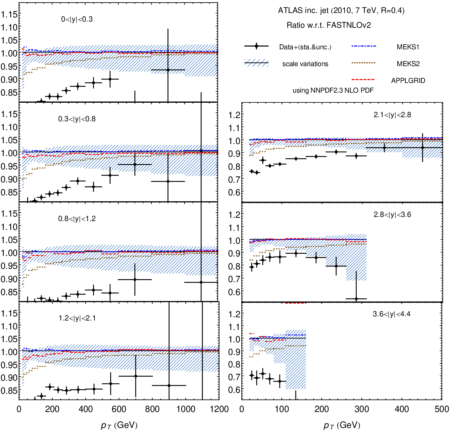
The MEKS cross sections are obtained with the scales equal to the individual jet $p_{T}^{\rm ind}$ (same as in FastNLO and denoted by MEKS1) or the hardest jet $p_{T}^{hard}$ in each event (MEKS2). In the MEKS1 convention, if the transverse momenta $\{p_{T}\}=\{p_{T}^{(1)},p_{T}^{(2)},p_{T}^{(3)}\}$ of the jets in a three-jet event are ordered as $p_{T}^{(1)}>p_{T}^{(2)}>p_{T}^{(3)}$ , the event contributes cross section weights $w(\{p_{T}\},\mu=p_{T}^{(1)}),$ $w(\{p_{T}\},\mu=p_{T}^{(2)}),$ and $w(\{p_{T}\},\mu=p_{T}^{(3)})$ into the $p_{T}$ bins around $p_{T}^{(1)},$ $p_{T}^{(2)}$ , and $p_{T}^{(3)}$ , respectively. In the MEKS2 convention, the event contributes the same cross section weight $w(\{p_{T}\},\mu=p_{T}^{(1)})$ into all three bins.

The scale choice in APPLgrid sets $\mu_{R}$ and $\mu_{F}$ equal to the $p_{T}$ of the hardest jet in each rapidity bin. It coincides with the MEKS1 convention if all $p_{T}$ values fall into different rapidity bins, but will select the larger of the two $p_{T}$ values as the scale if two jets are in the same rapidity bin.

In Fig. 15, we can see that, at the largest $p_{T}$ values, all four predictions agree to within 1%. FastNLO and MEKS1 agree to about 1% even at low $p_{T}$ , apart from minor fluctuations caused by Monte-Carlo integration errors. Their agreement is not surprising, since FastNLO and MEKS1 follow the same scale choice.

At low $p_{T}$ , the APPLgrid event rate shows a systematic deficit of up to 4% compared to FastNLO, while the MEKS2 rate is even smaller in this region. This is the consequence of using the QCD scale that is equal or close to the hardest jet $p_{T}$ , which suppresses the cross section compared to other scale choices. The MEKS2 curve lies, for the most part, within the scale uncertainty band of the FastNLO prediction, with the exception of the $p_{T}<200$ GeV region. We conclude that the most up-to-date versions of the parton-level NLO programs show a very good agreement for the same scale choice. However, the scale dependence of the NLO cross section is an important systematic uncertainty, its magnitude is of the same order as the experimental correlated systematic errors. In Fig. 15, which shows the experimental data without the correlated systematic errors, the difference between the theoretical predictions $T_{k}$ and the unshifted central data values $D_{k}$ provides a crude estimate of the size of the correlated systematic error. As seen in the last section, the quality of the fit is very good, so the data and theory predictions can be brought into line using shifts of data corresponding to the size of the correlated errors, or less. In fact, it can be checked from the results in [55] that this is a reasonable approximation, especially at the highest $p_{T}$ values and the highest rapidity bins, where the systematic uncertainty is larger than the difference between $T_{k}$ and $D_{k}$ in Fig. 15. The scale uncertainty, defined as above, varies from about 15% of $T_{k}-D_{k}$ in the bins with the small rapidity to 40% at the largest $\left|y\right|$ . Hence, the contribution of the scale uncertainty is significant compared to the experimental systematic uncertainty, and reduces the sensitivity of LHC inclusive (di)jet production to different PDF models, particularly at the highest rapidities.⁹⁹ 9 Theoretical uncertainties should be treated in a completely different footing of experimental uncertainties, and in particular, should not be included in the $\chi^{2}$ definition. The issue of the proper inclusion of theory uncertainties in PDF analysis is beyond the scope of this paper, and thus we do not explore it further.

5.2 PDF dependence

As already seen in the previous section, all available PDF sets can fit well the current ATLAS jet data, which therefore does not provide much discrimination. However, there are still interesting features to pick out which will become more important for future data. Fig. 16 compares the corresponding NLO predictions made using APPLgrid and various NNLO PDFs: ABM11, CT10, HERA1.5, MSTW08, and NNPDF2.3. We take $\alpha_{s}(M_{Z})=0.119$ both in the hard cross sections and PDFs for all PDF sets. All the predictions are normalized to the central prediction based on the CT10 NNLO PDF set (with $\alpha_{s}=0.119$ ). For the NNPDF2.3 and CT10 sets, we show the 68% C.L. PDF uncertainties by the hatched bands. The CT10 central predictions are larger than NNPDF2.3 or MSTW2008, mainly due to the harder gluon distribution in the CT10 set. In general, predictions from different PDFs agree with each other within the range of PDF uncertainties, apart from ABM11, particularly at low rapidities. It is also instructive to compare the scale uncertainties shown in Fig. 15 with the PDF uncertainties shown in Fig. 16. In the low $p_{T}$ region, i.e. less than $p_{T}\sim 200$ GeV, the scale uncertainty of NLO predictions is comparable to, or even larger than, the PDF uncertainties from CT10. This is another indication that the scale uncertainty presents a limiting factor in the discrimination between the PDF sets, especially for PDFs which are already well-constrained, in this case by HERA data.

PDF set	$\chi^{2}/N_{pt}$	$\chi_{D}^{2}$	$\chi_{\lambda}^{2}$	$\lambda_{0,\rm lum}$
ABM11	0.81	44.4	28.5	-1.12
CT10	0.81	47.4	25.5	-1.76
CT10 NLO	0.94	54.0	30.6	-1.18
HERA1.5	0.85	50.7	25.8	-2.36
MSTW08	0.79	45.7	25.1	-2.00
NNPDF2.3	0.79	42.4	29.1	-1.88

Table 10:

\chi^{2}/N_{\rm pt}

values for the 2010 ATLAS single-inclusive jet data (

R=0.4

) computed according to Eq. (11) using FastNLO (version 2) and various NNLO PDF sets and the CT10 NLO set. The

\chi_{D}^{2}

and

\chi_{\lambda}^{2}

contributions to

\chi^{2}

from the data residuals and penalties for systematic shifts defined in Eqs. (12) and (13) are shown. The last column contains the best-fit luminosity parameter shift

\lambda_{0,\rm lum}

for each PDF set. We have used

\alpha_{s}=0.119

for all sets.

5.3 Systematic shifts in a fit to the ATLAS jet data

When the NLO theoretical predictions are compared to the ATLAS inclusive jet data without including the systematic errors, as in Fig. 15, one generally finds a very poor agreement for any PDF set. In this case, the $\chi^{2}$ value can reach several thousand units for a total of $N_{\rm pt}=90$ data points. The agreement is improved dramatically after the correlated systematic errors are considered. This can be done, e.g., by including a term with a correlation matrix $\beta_{k\alpha}$ into the log-likelihood function $\chi^{2}$ [77], as described in the appendix. We will use the definition of $\chi^{2}$ provided by Eq. (11), which introduces a normally distributed nuisance parameter $\lambda_{\alpha}$ (with the central value of zero and standard deviation of one) to characterize each of $N_{\lambda}$ correlated errors.

The ATLAS measurement provides $88$ sources of correlated systematic errors, including the luminosity error and the uncertainty in the nonperturbative correction. Each of these errors can cause variations (shifts) of the experimental points from their central values. In addition, each data point is affected by an uncorrelated systematic error, which is significant compared to the statistical error. When both uncorrelated and correlated systematic uncertainties are included into $\chi^{2}$ , the resulting $\chi^{2}/N_{\rm pt}$ values are less than $1$ for all considered NNLO PDFs, as shown in Table 10. In this comparison, $\chi^{2}$ is computed according to the procedure summarized in Sec. A.2 and numerically equivalent to Eq. (8). None of the PDF sets is preferred by these $\chi^{2}$ values. As one can see the $\chi^{2}$ values are extremely similar to those in the previous section, Tables 7 and 8, even though they are computed with a different code (FastNLO).

For each set of theoretical predictions $\{T_{k}\}$ , we can also determine the value $\lambda_{0\alpha}$ of each nuisance parameter that gives the best description of the data. It is found according to Eq. (14) once the $\{T_{k}\}$ values are known. In Eq. (11) for the total $\chi^{2}$ , we can identify two parts: $\chi_{D}^{2}$ containing contributions from the data residuals $d_{k}=(D_{k}^{\rm shifted}-T_{k})/s_{k}$ , where $D_{k}^{\rm shifted}=D_{k}-\sum_{\alpha}\beta_{k\alpha}\lambda_{0\alpha}$ ; and $\chi_{\lambda}^{2},$ which is a quadrature sum $\sum_{\alpha}\lambda_{\alpha}^{2}$ of the shifted nuisance parameters. We list $\chi_{D}^{2}$ and $\chi_{\lambda}^{2}$ separately in Table 10 and include histograms of the data residuals $d_{k}$ and best-fit parameters $\lambda_{0\alpha}$ in Figs. 17 and 18. In the histograms (which are shown here for CT10 NNLO and NNPDF2.3 NNLO PDFs, but are also representative of the histograms for the other NNLO PDF sets), the observed $d_{k}$ and $\lambda_{0\alpha}$ distributions are narrower than the standard normal distributions shown by the dotted curves. In other words, the fit to the 2010 ATLAS data is too good and can’t distinguish between the PDF sets. Most of 88 best-fit parameters $\lambda_{\alpha 0}$ are close to zero, i.e., they don’t contribute much to the improvement of $\chi^{2}$ . None of the best-fit parameters included in Fig. 18 has changed by more than 2.5 standard deviations.

At the Tevatron, some PDF sets required a shift in the data downwards due to the luminosity uncertainty by as much as 3-4 standard deviations in order to agree with the single-inclusive jet production data, cf. the appendix in Ref. [30]. In that paper, it was argued that such shifts are not strictly allowed. The luminosity is common to the data on the $Z$ and $W$ total cross sections and the $Z$ rapidity distribution, which are rather constraining, and for which the PDF predictions are consistent with the nominal luminosity, or even a shift in the data upwards due to the luminosity uncertainty. It should be a mandatory test of PDFs that they fit the Tevatron and LHC jet and vector boson production data simultaneously, while the luminosity uncertainty is treated as completely correlated between the two types of measurement coming from the same experiment and the same data taking period. This has not been checked for all PDF sets and could help explain how some inconsistencies may arise. Note that Fig. 17 in Ref. [30] is of the same form as Fig. 18, but for Tevatron jet data. For the Tevatron inclusive jet data the distribution of the $\lambda_{0\alpha}$ is as expected, or even wider for poorly fitting PDFs, in contrast to those for ATLAS data.

The last column of Table 10 lists the best-fit values of the luminosity shift parameter in the ATLAS measurement, computed with the FastNLO code. Only one PDF set (HERA1.5 NNLO) requires a $2.4\sigma$ shift in the ATLAS luminosity. However, none of the PDF sets requires a luminosity shift by more than $3\sigma,$ suggesting that they are all compatible with the 2010 ATLAS jet data. This is despite the wide variety of predictions exhibited in Fig. 16. Clearly the improvement of the correlated systematic errors will be a priority for future data, since at present the shifts in data can accommodate quite dramatic differences in predictions without a large penalty in $\chi^{2}$ .

6 Combined uncertainties in Higgs production

In this section we discuss in somewhat greater detail PDF and $\alpha_{s}$ uncertainties for Higgs production via gluon fusion at the LHC, and specifically how PDF updates affect results obtained using the PDF4LHC recommendation [78] for the determination of PDF+ $\alpha_{s}$ uncertainties. At NLO this prescription entails finding the envelope of CT, MSTW and NNPDF PDF+ $\alpha_{s}$ uncertainty bands, each obtained with a different choice for the central value of $\alpha_{s}$ . The outer bands of the envelope are taken as the upper and lower limits of uncertainty, and the midpoint value as the best prediction. When the prescription was published, of the three PDF sets included in the prescription, only MSTW was available at NNLO. The NNLO prescription recommended taking the MSTW08 prediction as the central value, while rescaling the MSTW08 uncertainty by a factor determined comparing at NLO the MSTW08 uncertainty to the envelope uncertainty.

The NNLO cross section for Higgs production at LHC (8 TeV) is currently quoted by the Higgs Cross Section Working Group (HXSWG)¹⁰¹⁰ 10 https://twiki.cern.ch/twiki/bin/view/LHCPhysics/CERNYellowReportPageAt8TeV as

\sigma_{H}^{\rm NNLO}=19.52\pm 1.41~{\rm pb},\qquad(\pm 7.2\%~"{\rm PDF}+\alpha_{s}").

(3)

The HXSWG cross section numbers have been computed with the current (2010) PDF4LHC prescription, $m_{H}=125$ GeV, and de Florian-Grazzini code [79], which incorporates soft-gluon effects up to next-to-next-to-leading logarithmic accuracy on top of the exact NNLO calculation. Since in this work we use fixed order NNLO calculations as implemented in iHixs, the central values that we will quote cannot be compared directly to the HXSWG numbers. However, this should have a minimal effect on the percentage PDF+ $\alpha_{s}$ uncertainty.

We can thus investigate how the combined PDF+ $\alpha_{s}$ uncertainties would change if computed using an envelope prescription based on the most updated NNLO PDFs from the three global sets: NNPDF2.3, MSTW08 and CT10. Instead of the exact implementation of the PDF4LHC envelope, see e.g., Refs. [80, 1], for simplicity we use the following definition: we compute the combined PDF+ $\alpha_{s}$ uncertainties for the three PDF sets for $\alpha_{s}=0.117$ and $\alpha_{s}=0.119$ and let the maximum and minimum values of the cross section in this range define the envelope. Combined PDF and $\alpha_{s}$ uncertainties are obtained adding the two uncertainties in quadrature. The uncertainty on $\alpha_{s}$ is taken to be $\delta{\alpha_{s}}=0.0012$ at the 68% confidence level. The central value is taken as the midpoint of the envelope defined in this way.

This differs from the 2010 PDF4LHC prescription because in the latter the prediction from each of the three sets is obtained using a different value of $\alpha_{s}$ ( $\alpha_{s}=0.118$ for CTEQ, $\alpha_{s}=0.119$ for NNPDF and $\alpha_{s}=0.120$ for MSTW), and also because $\alpha_{s}$ and PDF uncertainties are added in quadrature instead of being determined exactly in the Hessian or Monte Carlo method (though in the Hessian method the two procedures are equivalent [cteqas]). The change in $\alpha_{s}$ range moves the central value a little, however, because the width of the $\alpha_{s}$ range is unchanged the uncertainty is not affected significantly. Adding the PDF and $\alpha_{s}$ uncertainties in quadrature reduces somewhat the MSTW08 uncertainty. Note also that the addition in quadrature was a simplification in the original PDF4LHC prescription. We used it because we think it is more suitable for benchmarking (which is the goal of this paper) while asymmetric $\alpha_{s}$ uncertainties may be more accurate and thus better for phenomenology.

As in Sect. 3, the cross sections are computed at NNLO with the iHixs code [33]. The central scale has been taken to be $Q=m_{H}$ , which is the same choice used for the default predictions for Higgs production adopted by the Higgs Cross Section Working Group [34].

We begin by computing the envelope defined as above at NLO with the same NLO PDF sets of 2010 PDF4LHC prescription: CTEQ6.6, MSTW08, and NNPDF2.0. The corresponding results for $\alpha_{s}=0.117$ and $0.119$ are summarized in Table 11. The envelope is

\sigma^{\rm NLO}_{H}=13.98\pm 0.85~{\rm pb},\qquad(\pm 6.1\%~"{\rm PDF}+\alpha_{s}"),

(4)

so the uncertainty is a bit smaller than the current HXSWG result.

Next, we repeat the computation of the NLO envelope, but now with the most up-to-date PDF sets: CT10, MSTW08, and NNPDF2.3. Results are also summarized in Table 11, and lead to the envelope:

\sigma^{\rm NLO}_{H}=14.05\pm 0.86~{\rm pb},\qquad(\pm 6.1\%~"{\rm PDF}+\alpha_{s}").

(5)

so neither the central value nor the uncertainty change significantly. Note that the increase in the Higgs cross section using NNPDF2.3, as compared to NNPDF2.0, does not lead to an increase of the combined PDF+ $\alpha_{s}$ error since the CT10 prediction also increases by a similar amount.

Finally, using the NNLO cross sections from the most updated NNLO PDF sets, but otherwise using the same prescription as at NLO, we obtain

\sigma_{H}^{NNLO}=18.75\pm 1.24~~{\rm pb},\qquad(6.6\%~"{\rm PDF}+\alpha_{s}").

(6)

The combined PDF+ $\alpha_{s}$ error is thus essentially unchanged when going from NLO to NNLO, while the central value is within 2% from the MSTW2008 NNLO value of $18.45$ pb, which in the 2010 PDF4LHC prescription was taken as the central value.

2010 NLO PDFs
$\alpha_{S}(M_{Z})$	NNPDF2.0	MSTW08	CTEQ6.6
0.117	14.04 $\pm$ 0.20 $\pm$ 0.27	13.94 $\pm$ 0.22 $\pm$ 0.27	13.49 $\pm$ 0.27 $\pm$ 0.24
0.119	14.49 $\pm$ 0.21 $\pm$ 0.27	14.38 $\pm$ 0.23 $\pm$ 0.27	13.88 $\pm$ 0.28 $\pm$ 0.24

2012 NLO PDFs
$\alpha_{S}(M_{Z})$	NNPDF2.3	MSTW08	CT10
0.117	14.21 $\pm$ 0.20 $\pm$ 0.25	13.94 $\pm$ 0.22 $\pm$ 0.27	13.57 $\pm$ 0.28 $\pm$ 0.26
0.119	14.61 $\pm$ 0.17 $\pm$ 0.25	14.38 $\pm$ 0.23 $\pm$ 0.27	14.00 $\pm$ 0.29 $\pm$ 0.26

2012 NNLO PDFs
$\alpha_{S}(M_{Z})$	NNPDF2.3	MSTW08	CT10
0.117	18.90 $\pm$ 0.20 $\pm$ 0.38	18.45 $\pm$ 0.24 $\pm$ 0.40	18.05 $\pm$ 0.36 $\pm$ 0.41
0.119	19.54 $\pm$ 0.25 $\pm$ 0.38	19.12 $\pm$ 0.25 $\pm$ 0.40	18.73 $\pm$ 0.37 $\pm$ 0.41

Table 11: The Higgs boson production cross section (in pb) in the gluon fusion channel, for

m_{H}=125

GeV at LHC 8 TeV. The two uncertainties shown in each case are the PDF and

\alpha_{s}

uncertainty.

These cross sections are plotted in Fig. 19 and Fig. 20, showing both the cross sections from each individual PDF set and the envelope.

In summary, neither the central value nor the uncertainty on the NLO prediction are significantly affected when replacing 2010 PDF with 2012 PDFs, and if the NLO PDF4LHC prescription is also used at NNLO, the combined PDF+ $\alpha_{s}$ uncertainty for the Higgs cross section moderately rises from 6.1% to 6.6% when going from NLO to NNLO.

In this respect, the gluon fusion channel with $m_{H}=125$ GeV is an unusually unlucky case: for most standard candle processes, as well as for other Higgs production modes, and even for gluon fusion, but with other values of the Higgs mass, the uncertainties decrease when going from 2010 NLO PDFs to 2012 NNLO PDFs, as it is clear from comparing the luminosity plots of Section 2 with analogous plots from previous benchmarks [1, 2].

To illustrate this explicitly, we compare in Fig. 21 predictions for $W^{+}$ boson production based on NLO PDFs, both from 2010 and from 2012, and 2012 NNLO PDFs from CT, MSTW and NNPDF. The improved agreement of the PDF sets when going from 2010 to 2012 PDFs is clear: the relative PDF+ $\alpha_{s}$ uncertainty, defined with the same prescription as for the Higgs cross section, goes down from $\Delta_{\rm PDF+\alpha_{s}}=5.3\%$ to $\Delta_{\rm PDF+\alpha_{s}}=3.3\%$ , i.e. from more than twice the MSTW2008 uncertainty (sometimes used as a simple approximation to the full envelope) to about 1.5 times the MSTW2008 uncertainty. Several factors contribute to this improvement, which include for instance the adoption of a GM-VFN scheme in NNPDF2.1 and a more similar choice of data sets in the different fits. Similar improvements are expected in all quark-initiated cross sections.

7 Conclusions and outlook

In this paper we have presented an updated benchmark comparison of the most recent NNLO PDF sets from the ABM, CT, HERAPDF, MSTW and NNPDF collaborations. We have compared PDFs, parton luminosities, LHC inclusive cross sections and differential distributions, always consistently for a common value of $\alpha_{s}$ .

Our main result is that the agreement between the most recent CT, MSTW and NNPDF NNLO parton distributions is at least as good as it was at NLO, and in many cases there is a clear improvement, in that the spread of predictions from different groups is reduced significantly. The HERAPDF1.5 NNLO central values are generally in good agreement with those of CT, MSTW and NNPDF, but with rather larger uncertainties due to the smaller dataset that HERAPDF uses. We find no evidence for tension between the HERA-only PDF sets and the PDF sets based on global data sets. It is interesting to observe that at NLO the HERAPDF1.5 set has smaller uncertainty and a more significant disagreement with other sets. The improvement in methodology in the HERAPDF1.5 NNLO analysis seems to not only to enlarge the uncertainty, but also to bring the central values more in line with the other sets.

We find that in several cases ABM11 disagrees with CT, MSTW and NNPDF both for PDFs and LHC cross sections, even when a common value of $\alpha_{s}$ is used. For the ABM11 default $\alpha_{s}(M_{Z})=0.1134$ value, many of these differences with other sets would further increase (though the vector boson production predictions would become more similar). We have discussed some of the possible explanations of these differences. A plausible explanation seems to be the use of the FFN scheme instead of the GM-VFN scheme used by the other groups, together with the absence of collider data in the ABM11 fit [30]. Other, perhaps less likely explanations, include the presence of higher twist contributions in the ABM PDF determination. We have also shown (cf. the end of Sect. 3) that the 8 TeV LHC data on total inclusive cross sections tend to disfavor ABM11, especially in top quark pair production for the default ABM11 $\alpha_{s}$ value, though experimental uncertainties are not yet precise enough to allow for a decisive discrimination.

For Higgs production via gluon-gluon fusion, we have shown that the combined PDF+ $\alpha_{s}$ uncertainties obtained from the envelope of CT, MSTW and NNPDF sets at NNLO are very similar to those obtained at NLO, which in turn are unchanged if 2012 instead of 2010 PDFs are used. For several other LHC processes (in particular quark-initiated processes) the NNLO combined PDF+ $\alpha_{s}$ uncertainty is smaller than the 2010 NLO result.

We would like to emphasize that we are not advocating here any new prescription to combine PDF sets, but only exploring the robustness of the original (2010) recommendation with respect to the update of its PDF sets. It is the task of the PDF4LHC Steering Committee to provide official updated recommendations for the use of PDFs in the comparisons with LHC data.

Available LHC data is already providing important information on PDFs, and future LHC data will provide even more stringent constraints. Such constraints will come from more precise measurements of already available processes (such as vector boson production and jet production), measurements of new PDF sensitive differential distributions (such as low-mass Drell-Yan pair, $W+$ charm, $t\bar{t}$ , or single-top production), as well as new ways of combining the existing data (such as ratios of LHC cross sections at different center-of-mass energies [57]).

Here we have presented only a small subset of all the available plots. A complete repository of all available plots is

http://nnpdf.hepforge.org/html/pdfbench/catalog ,

where in particular we provide

•

Comparisons of PDFs and parton luminosities at NLO and NNLO, for $\alpha_{s}(M_{Z})=0.117$ and 0.119.
•

Comparisons of PDFs at a low scale of 2 GeV², and as ratios with respect to a reference set for an LHC scale of $10^{4}$ GeV².
•

Comparison of PDFs to all the relevant LHC data from ATLAS, CMS and LHCb at NNLO, for $\alpha_{s}(M_{Z})=0.117$ and 0.119.
•

PDF dependence of benchmark cross sections.

Acknowledgments
We are grateful to Marco Zaro for providing the VBF results with the VBF@NNLO program. We would like to thank Alan Martin, Jon Pumplin, James Stirling, and Graeme Watt for discussions. This work is supported by the U.S. National Science Foundation under Grant No. PHY-0855561, the U.S. DOE Early Career Research Award DE-SC0003870, and by Lightner-Sams Foundation. J. R. is supported by a Marie Curie Intra–European Fellowship of the European Community’s 7th Framework Programme under contract number PIEF-GA-2010-272515. The work of R. S. T. is supported partly by the London Centre for Terauniverse Studies (LCTS), using funding from the European Research Council via the Advanced Investigator Grant 267352.

Appendix A Definitions of $\chi^{2}$

The value of the $\chi^{2}$ estimator depends on the assumed functional form for $\chi^{2}$ in the presence of experimental correlated systematic uncertainties. In this appendix, we document the various definitions of the $\chi^{2}$ function adopted in this paper and the numerical inputs that were used to obtain our results.

Statistical experimental errors are usually reported in the form of a list containing their absolute values, while for systematic errors the list gives relative values expressed as percentages of the central value. Often the systematic errors are asymmetric, i.e. they have different positive and negative deviations. The covariance matrix $({\rm cov})_{ij}$ is calculated from this published information by following one of the methods described below. Needless to say it is important, when benchmarking the various PDF predictions, to state precisely how the covariance matrix was computed. On the other hand some experiments directly provide the covariance matrix rather than the list of systematic errors, and in this case no ambiguity is possible.

A.1 Definitions of $\chi^{2}$ with the covariance matrix

We can define the $\chi^{2}$ for a specific experiment with $N_{\rm pt}$ data points by

\chi^{2}=\sum_{i,j}^{N_{\rm pt}}(T_{i}-D_{i})({\rm cov^{-1}})_{ij}(T_{j}-D_{j}),

(7)

and use it as a figure of merit to judge the agreement between theory and data. The covariance matrix $({\rm cov})_{ij}$ used in this definition may be written as

({\rm cov})_{ij}=\delta_{ij}s_{i}^{2}+\left(\sum_{\alpha=1}^{N_{c}}\sigma^{(c)}_{i,\alpha}\sigma^{(c)}_{j,\alpha}+\sum_{\alpha=1}^{N_{\cal L}}\sigma_{i,\alpha}^{({\cal L})}\sigma_{j,\alpha}^{({\cal L})}\right)D_{i}D_{j},

(8)

where $i$ and $j$ run over the experimental points ( $i,j=1,...,N_{\rm pt}$ ), $D_{i}$ are the measured central values, and $T_{i}$ the corresponding theoretical predictions computed with a given set of PDFs. This covariance matrix depends on uncorrelated uncertainties $s_{i}$ , constructed by adding the statistical and uncorrelated systematic uncertainties in quadrature; $N_{\cal L}$ multiplicative normalization uncertainties, $\sigma_{i,\alpha}^{({\cal L})}$ ; and $N_{c}$ other correlated systematic uncertainties, expressed for convenience in the above equation in terms of their relative values $\sigma^{(c)}_{i,\alpha}$ . The total number of correlated uncertainties is thus $N_{\lambda}=N_{\cal L}+N_{c}$ . Asymmetric systematic uncertainties provided by the experiments must be symmetrized to use this expression. We symmetrize them by averaging, $\sigma^{(c)}_{i,\alpha}={\textstyle{1\over 2}}(\sigma^{(c),+}_{i,\alpha}+\sigma^{(c),-}_{i,\alpha})$ .

Note that it is important when fitting to distinguish between additive uncertainties (where the experimentalists have determined a absolute shift in the observable due to a systematic uncertainty) and multiplicative uncertainties (where the experimentalists have determined a relative shift, as a fraction of the measured observable). In particular it is important not to mistake an additive uncertainty for a multiplicative one just because it is presented multiplicatively (as are the correlated systematics in Eq. (8), where the absolute shift in data point $i$ from systematic uncertainty $\alpha$ is written as $\sigma^{(c)}_{i,\alpha}D_{i}$ ). Correlated systematics which are truly multiplicative should of course be treated in the same way as the normalization uncertainty.

This distinction is important because if Eq. (8) were used as a figure of merit in an actual PDF fit, it would result in a D’Agostini bias of the multiplicative uncertainties [81]. However it is a suitable objective criteria for comparing a posteriori the various predictions from the different PDF sets that are discussed here, and we have used it as such throughout the body of this paper.

An alternative definition of the covariance matrix is the $t_{0}$ -prescription [81], where a fixed theory prediction $T_{i}^{(0)}$ (e.g., the final theory prediction from a previous fit) is used to define the normalization contribution to the $\chi^{2}$ . In the $t_{0}$ -prescription the covariance matrix is thus

({\rm cov})_{ij}=\delta_{ij}s_{i}^{2}+\sum_{\alpha=1}^{N_{c}}\sigma^{(c)}_{i,\alpha}\sigma^{(c)}_{j,\alpha}D_{i}D_{j}+\sum_{\alpha=1}^{N_{\cal L}}\sigma_{i,\alpha}^{({\cal L})}\sigma_{j,\alpha}^{({\cal L})}T^{(0)}_{i}T^{(0)}_{j}.

(9)

This definition has the advantage of avoiding the D’Agostini bias from multiplicative normalization uncertainties when performing a PDF fit.

When the breakdown into additive and multiplicative uncertainties is not provided by the experiment, one may use $T_{i}^{(0)}$ to compute all systematic uncertainties, to give an ‘extended- $t_{0}$ ’ prescription:

({\rm cov})_{ij}=\delta_{ij}s_{i}^{2}+\left(\sum_{\alpha=1}^{N_{c}}\sigma^{(c)}_{i,\alpha}\sigma^{(c)}_{j,\alpha}+\sum_{\alpha=1}^{N_{\cal L}}\sigma_{i,\alpha}^{({\cal L})}\sigma_{j,\alpha}^{({\cal L})}\right)T^{(0)}_{i}T^{(0)}_{j}.

(10)

This prescription rescales by $T_{i}^{(0)}$ all multiplicative uncertainties (associated with the normalization or not), but also modifies the additive uncertainties given by the experiment in a mild way consistent with their overall uncertainty. We will see below that the $t_{0}$ covariance matrix Eq. (9) and the extended- $t_{0}$ covariance matrix Eq. (10) generally produce lower $\chi^{2}$ values than the experimental definition in Eqs. (8) for datasets with substantial systematic uncertainties.

In summary, we consider in this appendix three possible definitions of the covariance matrix:

$\displaystyle({\rm cov})_{ij}$ $\displaystyle=$ $\displaystyle\delta_{ij}s_{i}^{2}+\left(\sum_{\alpha=1}^{N_{c}}\sigma^{(c)}_{i,\alpha}\sigma^{(c)}_{j,\alpha}+\sum_{\alpha=1}^{N_{\cal L}}\sigma_{i,\alpha}^{({\cal L})}\sigma_{j,\alpha}^{({\cal L})}\right)D_{i}D_{j}\,,\quad"{\rm Exp}"$ $\displaystyle({\rm cov})_{ij}$ $\displaystyle=$ $\displaystyle\delta_{ij}s_{i}^{2}+\sum_{\alpha=1}^{N_{c}}\sigma^{(c)}_{i,\alpha}\sigma^{(c)}_{j,\alpha}D_{i}D_{j}+\sum_{\alpha=1}^{N_{\cal L}}\sigma_{i,\alpha}^{({\cal L})}\sigma_{j,\alpha}^{({\cal L})}T^{(0)}_{i}T^{(0)}_{j}\,,\quad"t_{0}"$ $\displaystyle({\rm cov})_{ij}$ $\displaystyle=$ $\displaystyle\delta_{ij}s_{i}^{2}+\left(\sum_{\alpha=1}^{N_{c}}\sigma^{(c)}_{i,\alpha}\sigma^{(c)}_{j,\alpha}+\sum_{\alpha=1}^{N_{\cal L}}\sigma_{i,\alpha}^{({\cal L})}\sigma_{j,\alpha}^{({\cal L})}\right)T^{(0)}_{i}T^{(0)}_{j}\ ,\quad"{\rm Extended}-t_{0}"$

A.2 Definitions of $\chi^{2}$ with shift parameters

An alternative, yet numerically equivalent, representation for the $\chi^{2}$ function has been used in the jet benchmarking exercise of Sec. 5, following the method traditionally adopted in the CTEQ and MSTW PDF fits for jet and some other data sets. In this representation, the $\chi^{2}$ figure of merit for goodness-of-fit to an experiment with correlated systematic uncertainties is expressed as [77]

\chi^{2}(\{a\},\{\lambda\})=\chi^{2}_{D}+\chi^{2}_{\lambda},

(11)

where

\chi^{2}_{D}\equiv\sum_{k=1}^{N_{\rm pt}}{{1}\over{s_{k}^{2}}}\left(D_{k}-T_{k}-\sum_{\alpha=1}^{N_{\lambda}}\beta_{k,\alpha}\lambda_{\alpha}\right)^{2},

(12)

and

\chi^{2}_{\lambda}\equiv\sum_{\alpha=1}^{N_{\lambda}}\lambda_{\alpha}^{2},

(13)

using the same notation as in the previous section, where the $\beta_{k,\alpha}$ are the absolute correlated uncertainties. Systematic uncertainties associated with $N_{\lambda}$ sources may now induce correlated variations (shifts) in the experimental data points. Their effect is approximated by including a sum $\sum_{\alpha}\beta_{k,\alpha}\lambda_{\alpha}$ dependent on the correlation matrix $\beta_{k,\alpha}$ ( $k=1,...,N_{\rm pt}$ ; $\alpha=1,...,N_{\lambda}$ ) and stochastic nuisance parameters $\lambda_{\alpha},$ with one nuisance parameter assigned to every source of the systematic uncertainty. By a common assumption, each $\lambda_{\alpha}$ follows the standard normal distribution. Its deviation from $\lambda_{\alpha}=0$ incurs a penalty contribution $\lambda_{\alpha}^{2}$ to $\chi^{2}$ . Under this assumption the minimum of $\chi^{2}$ with respect to $\lambda_{\alpha}$ can be found algebraically, since the dependence on $\lambda_{\alpha}$ is quadratic [77].

We can solve for the best-fit values $\lambda_{0\alpha}$ of the nuisance parameters to find

\lambda_{0\alpha}=\sum_{i=1}^{N_{\rm pt}}{{D_{i}-T_{i}}\over{s_{i}}}\sum_{\delta=1}^{N_{\lambda}}\mathcal{A}_{\alpha\delta}^{-1}{{\beta_{i,\delta}}\over{s_{i}}},

(14)

with

\mathcal{A_{\alpha\beta}}=\delta_{\alpha\beta}+\sum_{k=1}^{N_{\rm pt}}{{\mathbb{\beta}_{k,\alpha}\beta_{k,\beta}}\over{s_{k}^{2}}}.

(15)

When these $\lambda_{0\alpha}$ values are substituted into Eq. (13), one obtains the usual expression Eq. (7) for the $\chi^{2}$ , with

({\rm cov})_{ij}^{-1}=\left[{{\delta_{ij}}\over{s_{i}^{2}}}-\sum_{\alpha,\beta=1}^{N_{\lambda}}{{\beta_{i,\alpha}}\over{s_{i}^{2}}}\mathcal{A}_{\alpha\beta}^{-1}{{\beta_{j,\beta}}\over{s_{j}^{2}}}\right],

(16)

the inverse of

({\rm cov})_{ij}\equiv s_{i}^{2}\delta_{ij}+\sum_{\alpha=1}^{N_{\lambda}}\beta_{i,\alpha}\beta_{j,\alpha}.

(17)

If the absolute correlation $\beta_{i,\alpha}$ is related to the relative correlation $\sigma_{i,\alpha}$ by multiplying by the experimental central values for both $\sigma_{i\alpha}^{(c)}$ and $\sigma_{i\alpha}^{(\cal L)}$ ,

\beta_{i,\alpha}=\sigma_{i,\alpha}D_{i},

(18)

the expression in Eq. (17) coincides with the covariance matrix introduced earlier in Eq. (8). It is equivalent to the usual definition Eq. (8), but also contains explicit information about the values of the systematic parameters $\lambda_{0\alpha}$ at the best fit.

If instead of Eq. (18) we set

\beta_{i,\alpha}=\sigma_{i,\alpha}T^{(0)}_{i},

(19)

we recover the extended- $t_{0}$ $\chi^{2}$ in Eq. (10). Finally, using Eq. (18) to find $\sigma_{i\alpha}^{(c)}$ and Eq. (19) to find $\sigma_{i\alpha}^{(\cal L)}$ , we recover the $t_{0}$ definition in Eq. (9). Thus the $\chi^{2}$ values in the shift method as defined here are entirely equivalent to the methods based on direct inversion of the covariance matrix in Sec. A.1.

A.3 Impact on LHC cross sections

Numerical comparisons of the different $\chi^{2}$ prescriptions will depend on the exact procedure used to determine $s_{i}$ and $\sigma_{i,\alpha}$ . For example, in the comparisons to the ATLAS jet data in Sec. 5, we compute $\beta_{k,\alpha}$ using Eq. (18) (equivalent to Eq. (8)), averaging any asymmetric errors. Given the large number of independent systematic parameters ( $N_{\lambda}=88$ ), the asymmetry of some nuisance parameters is not expected to significantly bias the resulting PDFs, which has been confirmed by computing the $\chi^{2}$ tables using the same $\chi^{2}$ definition, but following alternative error symmetrization procedures. In all cases examined, the choice of the symmetrization procedure had a smaller effect on $\chi^{2}$ for the ATLAS jet data than the choice of the $\chi^{2}$ definition.

We have also checked numerically that the covariance matrix definitions described in Sec. A.1 and the corresponding shift definitions described in Sec. A.2 give the same results when implemented numerically (as they should). Thus for the remainder of this section we will focus on the difference between the three definitions of the covariance matrix described in Sec. A.1.

	NLO PDFs, $\alpha_{s}=0.119$
Dataset	NNPDF2.3	MSTW08	CT10	ABM11	HERAPDF1.5
ATLAS $W,Z$ (Exp)	1.268	2.004	1.062	1.558	1.747
ATLAS $W,Z$ ( $t_{0}$ )	1.292	2.024	1.026	1.487	1.676
CMS $W$ el asy (Exp)	0.820	4.690	1.419	1.915	0.687
CMS $W$ el asy ( $t_{0}$ )	0.820	4.690	1.419	1.915	0.687
LHCb $W$ (Exp)	0.670	0.907	1.064	2.328	4.125
LHCb $W$ ( $t_{0}$ )	0.662	0.896	1.046	2.298	4.100
ATLAS jets (Exp)	0.999	0.974	1.350	1.342	1.106
ATLAS jets ( $t_{0}$ )	0.836	0.825	1.234	1.317	1.032

Table 12: The

\chi^{2}/N_{\rm pt}

values for the available LHC data with published correlated uncertainties, computed using the five PDF sets considered. The experimental (“Exp”) definition of

({\rm cov})_{ij}

in Eq. (8) is compared to the

t_{0}

definition in Eq. (9). Theoretical predictions have been computed at NLO with APPLgrid for a common value of the strong coupling

\alpha_{s}\left(M_{Z}\right)=0.119

. The central PDF set of each collaboration has been used to compute the

t_{0}

matrix for the corresponding set.

In Table 12, we compare the default ’experimental’ definition of the covariance matrix used in the paper (cf. Eq. (8)) and the $t_{0}$ definition of Eq. (9). In this case, recent LHC measurements for $W$ , $Z$ , and jet production are compared to NLO predictions with five PDF sets and $\alpha_{s}=0.119$ . Results at NNLO and for other values of the strong coupling are qualitatively similar. One can see that the $t_{0}$ definition leads to smaller numerical values of $\chi^{2}$ for all PDF sets considered, especially in experiments with sizable normalization contributions, though it is also clear that the qualitative comparison between PDF sets in Sect. 4 is not affected by this alternative definition.

Similarly, the experimental definition is compared with the extended- $t_{0}$ definition in the case of ATLAS jet production with $R=0.4$ in Table 13. The comparisons are made for the NLO PDF sets, $\alpha_{s}$ values, and computer codes specified in the table. Three columns of $\chi^{2}/N_{\rm pt}$ are shown, corresponding to the ’experimental’ definition realized according to Eqs. (17) and (18) in column 1; and the extended- $t_{0}$ definition based on Eqs. (17) and (19), with the reference cross sections $T^{(0)}_{i}$ found using the central CT10 NLO in column 2 and NNPDF2.3 NLO PDFs in column 3.¹¹¹¹ 11 The “exp” NNPDF2.3 entry with APPLgrid in this table is numerically equivalent to the corresponding “exp” entry in the next-to-the last row of Table 12. In this case, the the $\chi^{2}/N_{\rm pt}$ values in columns 2 and 3 are noticeably lower than in column 1. They are not exactly the same in columns 2 and 3, indicating that $\chi^{2}$ also depends to some extent on the PDF that was used to compute $T^{(0)}$ . However this difference is much smaller than the difference between results using different codes, or different scale choices.

NLO PDF	$\alpha_{s}$	Code	$({\rm cov})_{ij}$ definition
			Exp	Ext. $t_{0}$	Ext. $t_{0}$
				CT10	NNPDF2.3
CT10	0.118	FastNLO	0.95	0.55	0.60
CT10	0.118	MEKS1	1.00	0.57	0.61
CT10	0.118	MEKS2	0.89	0.55	0.59
NNPDF2.3	0.119	FastNLO	0.87	0.60	0.57
NNPDF2.3	0.119	MEKS1	0.90	0.58	0.55
NNPDF2.3	0.119	MEKS2	0.78	0.54	0.53
NNPDF2.3	0.119	APPLgrid	1.00	0.64	0.62

Table 13: The

\chi^{2}/N_{\rm pt}

values for the ATLAS inclusive jet production data obtained with the experimental and extended-

t_{0}

definitions of the

\chi^{2}

function. The cross sections are computed at NLO using the specified NLO PDFs,

\alpha_{s}

values, and the following codes: FastNLO, MEKS with

\mu_{F,R}

equal to the individual jet

p_{T}

(MEKS1) or

p_{T}

of the hardest jet (MEKS2), and APPLgrid.

The comparisons of the three covariance matrix definitions in the two tables indicate that, for the ATLAS jet data, the difference in the corresponding $\chi^{2}$ values is quite large. Note that in this comparison, the $t_{0}$ covariance matrix treats only the normalization of these data as multiplicative, whereas the extended- $t_{0}$ treats all systematic uncertainties as multiplicative. Hence, it is always important to know when performing a fit whether a correlated error as determined by the experimentalists is multiplicative (hence, susceptible to the d’Agostini bias) or additive, since this will affect the impact of that data on the fit.

References

[1] G. Watt, JHEP 1109 (2011) 069, arxiv:1106.5788.
[2] G. Watt, Nucl.Phys.Proc.Suppl. 222-224 (2012) 61, arxiv:1201.1295.
[3] S. Alekhin, J. Blumlein and S. Moch, (2012), arxiv:1202.2281.
[4] S. Alekhin et al., Phys. Rev. D81 (2010) 014032, arxiv:0908.2766.
[5] S. Alekhin and S. Moch, Phys. Lett. B699 (2011) 345, arxiv:1011.5790.
[6] P. Nadolsky et al., (2012), arxiv:1206.3321.
[7] H.L. Lai et al., Phys. Rev. D82 (2010) 074024, arxiv:1007.2241.
[8] M. Guzzi et al., Phys.Rev. D86 (2012) 053005, arxiv:1108.5112.
[9] H1 and ZEUS Collaborations, V. Radescu, PoS ICHEP2010 (2010) 168.
[10] ZEUS Collaboration, H1 Collaboration, A. Cooper-Sarkar, PoS EPS-HEP2011 (2011) 320, arxiv:1112.2107.
[11] H1 Collaboration, F. Aaron et al., JHEP 1209 (2012) 061, arxiv:1206.7007.
[12] ZEUS Collaboration, A. Cooper Sarkar, (2012), arxiv:1208.6138.
[13] R.D. Ball et al., Nucl.Phys. B867 (2013) 244, arxiv:1207.1303.
[14] S. Forte et al., Nucl. Phys. B834 (2010) 116, arxiv:1001.2312.
[15] A.D. Martin et al., Eur. Phys. J. C63 (2009) 189, arxiv:0901.0002.
[16] R. Thorne et al., PoS DIS2010 (2010) 052, arxiv:1006.2753.
[17] G. Watt and R. Thorne, JHEP 1208 (2012) 052, arxiv:1205.4024.
[18] A.D. Martin et al., (2012), arxiv:1211.1215.
[19] P. Jimenez-Delgado and E. Reya, Phys. Rev. D80 (2009) 114011, arxiv:0909.1711.
[20] Particle Data Group, J. Beringer et al., Phys.Rev. D86 (2012) 010001.
[21] S. Lionetti et al., Phys. Lett. B701 (2011) 346, arxiv:1103.2369.
[22] R.D. Ball et al., Phys.Lett. B707 (2012) 66, arxiv:1110.2483.
[23] A.D. Martin et al., Eur. Phys. J. C64 (2009) 653, arxiv:0905.3531.
[24] ATLAS Collaboration, G. Aad et al., Phys.Rev.Lett. (2012), arxiv:1203.4051.
[25] J.M. Campbell, J.W. Huston and W.J. Stirling, Rept. Prog. Phys. 70 (2007) 89, hep-ph/0611148.
[26] R. Thorne, Phys. Rev. D86 (2012) 074017, arxiv:1201.6180.
[27] A.M. Cooper-Sarkar, (2007), arxiv:0709.0191.
[28] R. Thorne, Phys.Rev. D73 (2006) 054019, hep-ph/0601245.
[29] The NNPDF Collaboration, R.D. Ball et al., Nucl. Phys. B809 (2009) 1, arxiv:0808.1231.
[30] R. Thorne and G. Watt, JHEP 1108 (2011) 100, arxiv:1106.5789.
[31] A.D. Martin et al., Phys.Lett. B443 (1998) 301, hep-ph/9808371.
[32] A.D. Martin et al., Eur. Phys. J. C35 (2004) 325, hep-ph/0308087.
[33] C. Anastasiou et al., JHEP 1112 (2011) 058, 1107.0683.
[34] LHC Higgs Cross Section Working Group, S. Dittmaier et al., (2011), arxiv:1101.0593.
[35] P. Bolzoni et al., Phys.Rev.Lett. 105 (2010) 011801, arxiv:1003.4451.
[36] O. Brein, A. Djouadi and R. Harlander, Phys.Lett. B579 (2004) 149, hep-ph/0307206.
[37] O. Brein, R.V. Harlander and T.J. Zirke, (2012), arxiv:1210.5347.
[38] J. Campbell and R.K. Ellis, Phys. Rev. D65 (2002) 113007, hep-ph/0202176.
[39] C. Anastasiou et al., Phys. Rev. D69 (2004) 094008, hep-ph/0312266.
[40] M. Czakon and A. Mitov, (2011), 1112.5675.
[41] P. Baernreuther, M. Czakon and A. Mitov, Phys.Rev.Lett. 109 (2012) 132001, 1204.5201.
[42] M. Cacciari et al., Phys.Lett. B710 (2012) 612, arxiv:1111.5869.
[43] M. Czakon and A. Mitov, (2012), arxiv:1210.6832.
[44] M. Czakon and A. Mitov, (2012), arxiv:1207.0236.
[45] M. Aliev et al., Comput. Phys. Commun. 182 (2011) 1034, arxiv:1007.1327.
[46] S. Moch, P. Uwer and A. Vogt, Phys.Lett. B714 (2012) 48, arxiv:1203.6282.
[47] CMS, 2012, CMS-PAS-TOP-12-007.
[48] CMS, 2012, CMS-PAS-TOP-12-022.
[49] CMS, 2012, CMS-PAS-SMP-12-011.
[50] ATLAS Collaboration, G. Aad et al., (2012), arxiv:1207.5644.
[51] D. d’Enterria and J. Rojo, Nucl.Phys. B860 (2012) 311, arxiv:1202.1762.
[52] ATLAS Collaboration, G. Aad et al., Phys.Rev. D85 (2012) 072004, arxiv:1109.5141.
[53] CMS Collaboration, S. Chatrchyan et al., Phys.Rev.Lett. 109 (2012) 111806, arxiv:1206.2598.
[54] LHCb Collaboration, R. Aaij et al., JHEP 1206 (2012) 058, arxiv:1204.1620.
[55] ATLAS Collaboration, G. Aad et al., Phys. Rev. D86 (2012) 014022, arxiv:1112.6297.
[56] ATLAS, (2012), ATLAS-CONF-2012-128.
[57] M.L. Mangano and J. Rojo, JHEP 1208 (2012) 010, arxiv:1206.3557.
[58] J. Campbell, R.K. Ellis and F. Tramontano, Phys. Rev. D70 (2004) 094012, hep-ph/0408158.
[59] T. Carli et al., Eur.Phys.J. C66 (2010) 503, arxiv:0911.2985.
[60] S. Catani, G. Ferrera and M. Grazzini, JHEP 1005 (2010) 006, arxiv:1002.3115.
[61] T. Kluge, K. Rabbertz and M. Wobisch, (2006), hep-ph/0609285.
[62] J. Gao et al., (2012), arxiv:1207.0513.
[63] NNPDF collaboration, R.D. Ball et al., Nucl. Phys. B849 (2011) 112, arxiv:1012.0836.
[64] NNPDF collaboration, R.D. Ball et al., Nucl.Phys. B855 (2012) 608, arxiv:1108.1758.
[65] J. Gao and P. Nadolsky, in preparation.
[66] S.D. Ellis, Z. Kunszt and D.E. Soper, Phys.Rev.Lett. 69 (1992) 1496.
[67] Z. Nagy, Phys.Rev.Lett. 88 (2002) 122003, hep-ph/0110315.
[68] Z. Nagy, Phys. Rev. D68 (2003) 094002, hep-ph/0307268.
[69] See http://projects.hepforge.org/fastnlo/form/index.html.
[70] fastNLO Collaboration, M. Wobisch et al., (2011), 1109.1310.
[71] N. Kidonakis and J.F. Owens, Phys. Rev. D63 (2001) 054019, hep-ph/0007268.
[72] S. Alioli et al., JHEP 1104 (2011) 081, arxiv:1012.3380.
[73] S. Hoeche and M. Schonherr, (2012), arxiv:1208.2815.
[74] S. Dittmaier, A. Huss and C. Speckner, (2012), arxiv:1210.0438.
[75] S. Moretti, M. Nolten and D. Ross, Phys.Rev. D74 (2006) 097301, hep-ph/0503152.
[76] The NNPDF collaboration, R.D. Ball et al., Nucl. Phys. B838 (2010) 136, arxiv:1002.4407.
[77] J. Pumplin et al., JHEP 07 (2002) 012, hep-ph/0201195.
[78] M. Botje et al., (2011), arxiv:1101.0538.
[79] D. de Florian, M. Grazzini and M. Grazzini, Phys.Lett. B718 (2012) 117, arxiv:1206.4133.
[80] F. Demartin et al., Phys. Rev. D82 (2010) 014002, arxiv:1004.0962.
[81] The NNPDF collaboration, R.D. Ball et al., JHEP 05 (2010) 075, arxiv:0912.2276.