跳到论文正文
W Papers独立论文阅读器 arXiv:1211.5128 论文正文 计算阅读时间 · 0%
引用这篇论文根据当前论文元数据生成,正式投稿前建议核对。


License: arXiv.org perpetual non-exclusive license
arXiv:1211.5128v1 [math.AP] 21 Nov 2012

Existence of quasipatterns solutions of the Swift-Hohenberg equation

Boele Braaksma ††thanks: University of Groningen, Department of Mathematics P.O. Box 800, 9700 AV Groningen, The Netherlands. E-mail : braaksma@rug.nl    Gérard Iooss ††thanks: Institut Universitaire de France-Laboratoire J.-A. Dieudonné U.M.R. 7351, Université de Nice - Sophia Antipolis, Parc Valrose 06108 Nice Cedex 02, France. E-mail : gerard.iooss@unice.fr    Laurent Stolovitch ††thanks: CNRS-Laboratoire J.-A. Dieudonné U.M.R. 7351, Université de Nice - Sophia Antipolis, Parc Valrose 06108 Nice Cedex 02, France. E-mail : stolo@unice.fr. Ce travail a bénéficié d’une aide de l’Agence Nationale de la Recherche portant la référence “ANR-10-BLAN 0102”
Abstract

We consider the steady Swift - Hohenberg partial differential equation. It is a one-parameter family of PDE on the plane, modeling for example Rayleigh - Bénard convection. For values of the parameter near its critical value, we look for small solutions, quasiperiodic in all directions of the plane and which are invariant under rotations of angle π/q\pi/q, q≥4q\geq 4. We solve an unusual small divisor problem, and prove the existence of solutions for small parameter values.

1 Introduction

In the present paper we study the existence of a special kind of stationnary solutions (i.e. independent of tt), bifurcating from 00 (i.e. tending towards zero when the parameter λ\lambda tends towards 00), called quasipatterns of the 2-dimensional Swift-Hohenberg PDE

∂u∂t=λ​u−(1+Δ)2​u−u3\frac{\partial u}{\partial t}=\lambda u-(1+\Delta)^{2}u-u^{3} (1)

where uu is the unknown real-valued function on some subset of ℝ+×ℝ2\mathbb{R^{+}\times\mathbb{R}}^{2}, Δ:=(∂2∂x12+∂2∂x22)\Delta:=\left(\frac{\partial^{2}}{\partial x_{1}^{2}}+\frac{\partial^{2}}{\partial x_{2}^{2}}\right) and λ\lambda is a parameter. These are two-dimensional patterns that have no translation symmetry and are quasiperiodic in any spatial direction.

Mathematical existence of quasipatterns is one of the outstanding problems in pattern formation theory. To our knowledge, hereafter is the first proof of existence of such quasipatterns of a PDE. Quasipatterns were discovered in nonlinear pattern-forming systems in the Faraday wave experiment [BCM92, EF94], in which a layer of fluid is subjected to vertical oscillations. Since their discovery, they have also been found in nonlinear optical systems, shaken convection and in liquid crystals (see references in [AG12]) . In spite of the lack of translation symmetry (in contrast to periodic patterns), the solutions are π/q\pi/q-rotation invariant for some integer qq (most often observed, 2​q2q is 88, 1010 or 1212).

In many of these experiments, the domain is large compared to the size of the pattern, and the boundaries appear to have little effect. Furthermore, the pattern is usually formed in two directions (x1x_{1} and x2x_{2}), while the third direction (zz) plays little role. Mathematical models of the experiments are therefore often posed with two unbounded directions, and the basic symmetry of the problem is E⁡(2)E(2), the Euclidean group of rotations, translations and reflections of the (x1,x2)(x_{1},x_{2}) plane.

The above model equation is the simplest pattern-forming PDE, and is extremely successful for describing primary bifurcations (the first symmetry breaking) of hydrodynamical instability problems such as the Rayleigh - Bénard convection. Its essential properties are that

i) the system is invariant under the group E⁡(2)E(2);

ii) the instability occurs for a certain critical value of the parameter (here λ=0\lambda=0) for which critical modes are given by wave vectors sitting on a circle of non zero radius (here the unit circle);

iii) the linear part is selfadjoint and contains the main derivatives.

In contrast to periodic patterns, quasipatterns do not fit into any spatially periodic domain and have Fourier expansions with wavevectors that live on a quasilattice (defined below). At the onset of pattern formation, the critical modes have zero growth rate but there are other modes on the quasilattice that have growth rates arbitrarily close to zero, and techniques that are used for periodic patterns cannot be applied. These small growth rates appear as small divisors, as seen below, and correspond at criticality (OPENλ=0)\lambda=0) to the fact that for the linearized operator at the origin (here −(1+Δ)2-(1+\Delta)^{2}), the 0 eigenvalue is not isolated in the spectrum, appearing as part of the continuous spectrum.

If a formal computation in powers of λ\sqrt{\lambda} is performed in this case without regard to its validity, this results in a possibly divergent power series in the parameter, and this approach does not lead to the existence of quasipattern solutions, but instead to approximate solutions up to an exponentially small error  [IR10].

In this work, we prove the existence of quasipattern solutions of the steady Swift-Hohenberg equations. Our result rests on the article [IR10] by G. Iooss and A.M. Rucklidge which settle the mathematical foundation of the problem such as the formulation of suitable functions spaces. We refer to the articles of Rucklidge [RR03, RS07] and Iooss-Rucklidge[IR10] for physical motivation as well as for the bibliography.

Refer to caption
Figure 1: Example 88-fold quasipattern after [IR10]. This is an approximate solution of the steady Swift–Hohenberg equation (2) with λ=0.1\lambda=0.1, computed by using Newton iteration to find an equilibrium solution truncated to wavenumbers satisfying |𝐤|≤5|\mathbf{k}|\leq\sqrt{5} and to the quasilattice Γ27\Gamma_{27} obtained with N𝐤≤27N_{\mathbf{k}}\leq 27.

1.1 Main result and sketch of the proof

The problem is to find a special kind of solutions defined on ℝ2\mathbb{\mathbb{R}}^{2} of the steady Swift-Hohenberg equation

(1+Δ)2​U−λ​U+U3=0.(1+\Delta)^{2}U-\lambda U+U^{3}=0. (2)

The parameter λ\lambda is supposed to be real and small in absolute value. The solutions we are interested in should tend towards zero as the parameter goes to zero.

We study equation (2) for λ>0\lambda>0. Namely, let Q=2​qQ=2q be an even integer and let 𝐤j=exp⁡i​π​(j−1)q\mathbf{k}_{j}=\exp\frac{i\pi(j-1)}{q}, j=1,…,2​qj=1,\ldots,2q be the 2​q2q unit vectors of the plane, identified with roots of unity. Let Γ\Gamma be the set of linear combinations of vectors 𝐤j\mathbf{k}_{j} with nonnegative integer coefficients. We look for the existence of a (nonzero) π/q\pi/q-rotation invariant solution of the form

U⁡(𝐱)=∑𝐤∈Γu(𝐤)​ei​𝐤.𝐱U(\mathbf{x})=\sum_{\mathbf{k}\in\Gamma}u^{(\mathbf{k})}e^{i\mathbf{k}.\mathbf{x}}

which belongs to a “Sobolev” like space ℋs\mathcal{H}_{s}, s≥0s\geq 0 :

‖U‖s2:=∑𝐤∈𝚪|u(𝐤)|2​(1+N𝐤2)s<+∞.\|U\|_{s}^{2}:=\sum_{\mathbf{k\in\Gamma}}|u^{(\mathbf{k)}}|^{2}(1+N_{\mathbf{k}}^{2})^{s}<+\infty.

The natural number N𝐤N_{\mathbf{k}} denotes the minimal length of the linear combinations of the 𝐤j\mathbf{k}_{j}’s needed to reach 𝐤\mathbf{k}.

We then show that such a solution exists indeed, for small positive parameters λ\lambda:

Theorem 1.

For any q≥4q\geq 4 and any s>q/2s>q/2, there exists λ0>0,\lambda_{0}>0, such that the steady Swift-Hohenberg equation for 0<λ<λ00<\lambda<\lambda_{0}, admits a quasipattern solution in ℋs\mathcal{H}_{s}, invariant under rotations of angle π/q.\pi/q. Moreover the asymptotic expansion of this solution is given by the formal series given in [IR10].

One of the main difficulty is that the linearized operator at W=0W=0, has an unbounded inverse. Indeed, it is easy to show that the eigenvalues of (1+Δ)2(1+\Delta)^{2} in ℋs{\cal H}_{s} are (1−|𝐤|2)2(1-|{\mathbf{k}}|^{2})^{2} where 𝐤∈Γ{\mathbf{k}}\in{\Gamma}. These numbers accumulate in 00. It creates a small divisor problem, such that if λ>0\lambda>0 nothing can be said a priori about (1+Δ)2−λ​Id(1+\Delta)^{2}-\lambda\text{Id}. We use the first terms of the asymptotic expansion of the solution and change the unknown as U=Uϵ+ϵ4​WU=U_{{\epsilon}}+{\epsilon}^{4}W and λ=ϵ2​(λ2+λ4​ϵ2)\lambda={\epsilon}^{2}(\lambda_{2}+\lambda_{4}{\epsilon}^{2}) for some well chosen UϵU_{{\epsilon}} and positive λ2\lambda_{2}. Let ℒϵ{\cal L}_{{}_{\epsilon}} be the linear part at W=0W=0 of the nonlinear equation so obtained. For ϵ=0\epsilon=0, the operator ℒ0=(1+Δ)2\mathcal{L}_{0}=(1+\Delta)^{2} is a positive selfadjoint operator in ℋs\mathcal{H}_{s}. It is bounded from ℋs+4\mathcal{H}_{s+4} into ℋs\mathcal{H}_{s}, but it is not Fredholm, since its range is not closed. Its spectrum is an essential spectrum filling the half line [0,∞)[0,\infty). The set of eigenvalues is dense in the spectrum. The linear operator ℒϵ\cal L_{{\epsilon}} is the sum of ℒ0\mathcal{L}_{0} and a bounded operator (multiplication by a small function O⁡(ϵ2)O({\epsilon}^{2})) selfadjoint in ℋ0\mathcal{H}_{0}. If the range of ℒϵ\mathcal{L}_{{\epsilon}} were closed, a usual way to estimate the inverse of the selfadjoint operator ℒϵ\mathcal{L}_{{\epsilon}} in ℋ0\mathcal{H}_{0}, would be to estimate the distance from 00 to its numerical range (see [Kat95]) (containing the spectrum). Such estimate as

⟨ℒϵ​𝒰,𝒰⟩0≥c​ϵ2​‖U‖02{\langle\cal L_{{\epsilon}}U,U\rangle}_{0}\geq c{\epsilon}^{2}||U||_{0}^{2}

for a certain constant c>0c>0, cannot be proved here. So we need to study the linear operator in more details.

We show that there exists an orthogonal decomposition (depending on ϵ{\epsilon}) of the space ℋs=E0⊕E1⊕E2{\cal H}_{s}=E_{0}\oplus E_{1}\oplus E_{2}, s>q/2s>q/2, such that the solution of the equation ℒϵ​U=f{\cal L}_{{\epsilon}}U=f in ℋs{\cal H}_{s} can be computed and estimated from its E2E_{2}-component U2U_{2}. The latter is solution of a linear equation ℒϵ(2)​U2=f~{\cal L}^{(2)}_{{\epsilon}}U_{2}=\tilde{f}. The main part (with respect to powers of ϵ{\epsilon}) of that operator is an operator Λϵ\Lambda_{\epsilon}. When restricted to rotation invariant elements, it has a block-diagonal structure of fixed finite dimensional blocks. Then, it is possible to estimate all eigenvalues of these selfadjoint blocks. These eigenvalues have the form

(|𝐤|2−1)2+3​ϵ2+O⁡(ϵ4)(|{\mathbf{k}}|^{2}-1)^{2}+3{\epsilon}^{2}+O({\epsilon}^{4})

for 𝐤∈Γ{\mathbf{k}}\in{\Gamma}. One of the main feature is that they do not accumulate at the origin, and despite of the small divisor problem arising for ϵ=0\epsilon=0, we are able to give an upper bound in ℋ0\mathcal{H}_{0} of the inverse of Λϵ\Lambda_{\epsilon} of order 1/λ1/\lambda for nonzero λ\lambda. Then we extend this estimate in ℋs\mathcal{H}_{s} for s>q/2s>q/2. Finally, we use a variant of the implicit function theorem to conclude to the existence of quasipatterns solutions.

Remark 2.

If the coefficient (3) of ϵ2{\epsilon}^{2} were negative, then the operator could have again small divisors. Then the proof of the existence would have been much more involved. At that point, solving the nonlinear problem in U2U_{2} would have required the use of a version of Nash-Moser theorem such as those developed by J. Bourgain, W. Craig, M. Berti and al. (see for instance [Bou95, Cra00, BBP10, Ber07]). Their main feature is the use of the good separation property of the “singular sites” of the main linear operator. Indeed, we can show that the operator (1+Δ)2(1+\Delta)^{2} does have this property.

Remark 3.

For λ<0\lambda<0 the solution U=0U=0 is isolated in an open ball of radius |λ|\sqrt{|\lambda|}, as it is easily deduced from the following estimate

‖[(1+Δ)2−λ]−1‖≤|λ|−1||[(1+\Delta)^{2}-\lambda]^{-1}||\leq|\lambda|^{-1}

which holds in ℋs\mathcal{H}_{s}.

2 Analysis of the main part of the differential

2.1 Setting

In this section, we recall and improve some of the properties of the function spaces we use, as defined in [IR10].

Let Q=2​qQ=2q, q≥4q\geq 4 being an integer. Let us define the unit wave vectors (identifying ℂ\mathbb{C} with ℝ2\mathbb{R}^{2})

𝐤j:=ei​π​j−1q,j=1,…,2q.{\mathbf{k}}_{j}:=e^{i\pi\frac{j-1}{q}},\quad j=1,\ldots,2q. (3)

We define the quasilattice Γ⊂ℝ2{\Gamma}\subset{R}^{2} to be the set of points spanned by (nonnegative) integer linear combinations of the kjk_{j}’s :

𝐤m=∑j=12​qmj​𝐤j,𝐦=(m1,…,m2​q)∈ℕ2​q.{\mathbf{k}}_{m}=\sum_{j=1}^{2q}m_{j}{\mathbf{k}}_{j},\quad{\mathbf{m}}=(m_{1},\ldots,m_{2q})\in{N}^{2q}. (4)

We have 𝐤j=−𝐤j+q{\mathbf{k}}_{j}=-{\mathbf{k}}_{j+q}. Hence, we can write

𝐤m=∑j=1qmj′​𝐤j,{\mathbf{k}}_{m}=\sum_{j=1}^{q}m_{j}^{\prime}{\mathbf{k}}_{j},

where, mj′:=mj−mj+qm_{j}^{\prime}:=m_{j}-m_{j+q} belongs to ℤ{Z}. Thus,

|𝐤m|2=∑i,j=1qmi′​mj′​<𝐤i,𝐤j>.|{\mathbf{k}}_{m}|^{2}=\sum_{i,j=1}^{q}m_{i}^{\prime}m_{j}^{\prime}<{\mathbf{k}}_{i},{\mathbf{k}}_{j}>.

We then define, for any 𝐦∈ℕ2​q{\mathbf{m}}\in{N}^{2q} and 𝐤∈Γ{\mathbf{k}}\in{\Gamma},

|𝐦|:=∑jmj,N𝐤:=min⁡{|𝐦|:𝐤=𝐤m}.|{\mathbf{m}}|:=\sum_{j}m_{j},\quad N_{{\mathbf{k}}}:=\min\{|{\mathbf{m}}|:{\mathbf{k}}={\mathbf{k}}_{m}\}.

We have

Lemma 4.

[IR10][Lemma 4.1] For any 𝐤∈Γ{\mathbf{k}}\in{\Gamma}, we have :

  • •
    N𝐤+𝐤′≤N𝐤+N𝐤′,N−𝐤=N𝐤N_{{\mathbf{k}}+{\mathbf{k}}^{\prime}}\leq N_{{\mathbf{k}}}+N_{{\mathbf{k}}^{\prime}},\quad N_{-{\mathbf{k}}}=N_{{\mathbf{k}}} (5)
  • •
    |𝐤|≤N𝐤|{\mathbf{k}}|\leq N_{{\mathbf{k}}} (6)
  • •
    card⁡{𝐤|N𝐤=N}≤c1​(q)​Nq−1\operatorname{card}\{{\mathbf{k}}\;|\;N_{{\mathbf{k}}}=N\}\leq c_{1}(q)N^{q-1} (7)

    for some constant c1​(q)c_{1}(q) depending only on qq.

As in [IR10], we use function spaces defined as

ℋs={W=∑𝐤∈ΓW(𝐤)ei​𝐤⋅𝐱;||W||s2=∑𝐤∈Γ(1+N𝐤)2s|W(𝐤)|2<∞},{\mathcal{H}}_{s}=\left\{W=\sum_{\mathbf{k}\in\Gamma}W^{(\mathbf{k})}e^{i\mathbf{k}\cdot\mathbf{x}};\,||W||_{s}^{2}=\sum_{\mathbf{k}\in\Gamma}(1+N_{\mathbf{k}}{}^{2})^{s}|W^{(\mathbf{k})}|^{2}<\infty\right\}, (8)

which are Hilbert spaces with the scalar product

⟨W,V⟩s=∑𝐤∈Γ(1+N𝐤)2sW(𝐤)V¯(𝐤).\langle W,V\rangle_{s}=\sum_{\mathbf{k}\in\Gamma}(1+N_{\mathbf{k}}{}^{2})^{s}W^{(\mathbf{k})}\overline{V}^{(\mathbf{k})}. (9)
Lemma 5.

For s>q/2s>q/2, for any U∈ℋsU\in\mathcal{H}_{s} and any V∈ℋ0V\in\mathcal{H}_{0}, we have

‖U​V‖0≤cs​‖U‖s||V||0||UV||_{0}\leq c_{s}||U||_{s}||V||_{0}

for a certain constant cs>0.c_{s}>0.

Proof.

Using Cauchy-Schwarz inequality, we have

‖U​V‖02\displaystyle\|UV\|_{0}^{2} ≤\displaystyle\leq ∑𝐤∈Γ|∑𝐦∈ΓU(𝐦)​V(𝐤−𝐦)|2\displaystyle\sum_{{\mathbf{k}}\in{\Gamma}}\left|\sum_{{\mathbf{m}}\in{\Gamma}}U^{({\mathbf{m}})}V^{({\mathbf{k}}-{\mathbf{m}})}\right|^{2}
≤\displaystyle\leq ∑𝐤∈Γ(∑𝐦∈Γ|U(𝐦)|2​(1+N𝐦2)s)​(∑𝐦′∈Γ|V(𝐤−𝐦′)|2​(1+N𝐦′2)−s)\displaystyle\sum_{{\mathbf{k}}\in{\Gamma}}\left(\sum_{{\mathbf{m}}\in{\Gamma}}|U^{({\mathbf{m}})}|^{2}(1+N_{{\mathbf{m}}}^{2})^{s}\right)\left(\sum_{{\mathbf{m}}^{\prime}\in{\Gamma}}|V^{({\mathbf{k}}-{\mathbf{m}}^{\prime})}|^{2}(1+N_{{\mathbf{m}}^{\prime}}^{2})^{-s}\right)
≤\displaystyle\leq ‖U‖s2​(∑𝐤∈Γ|V(𝐤−𝐦′)|2)​Rs\displaystyle||U||_{s}^{2}\left(\sum_{{\mathbf{k}}\in{\Gamma}}|V^{({\mathbf{k}}-{\mathbf{m}}^{\prime})}|^{2}\right)R_{s}

where Rs:=∑𝐦′∈Γ(1+N𝐦′2)−sR_{s}:=\sum_{{\mathbf{m}}^{\prime}\in{\Gamma}}(1+N_{{\mathbf{m}}^{\prime}}^{2})^{-s}. This last sum converges if s>q/2s>q/2. Indeed, according to [IR10][(24)], card⁡{𝐤∈Γ|N𝐤=N}≤c⁡(q)​Nq−1\operatorname{card}\{{\mathbf{k}}\in{\Gamma}\;|\;N_{{\mathbf{k}}}=N\}\leq c(q)N^{q-1} for some constant c⁡(q)c(q). Hence ‖U​V‖02≤‖U‖s2​‖V‖02​Rs.\|UV\|_{0}^{2}\leq\|U\|_{s}^{2}\|V\|_{0}^{2}R_{s}.    

Lemma 6.

(Moser-Nirenberg type inequality) Let s,s′>q/2s,s^{\prime}>q/2 and let U,V∈ℋs∩ℋs′U,V\in\mathcal{H}_{s}\cap\mathcal{H}_{s^{\prime}}. Then,

‖U​V‖s≤C⁡(s,s′)​(‖U‖s​‖V‖s′+‖U‖s′​‖V‖s)\|UV\|_{s}\leq C(s,s^{\prime})(\|U\|_{s}\|V\|_{s^{\prime}}+\|U\|_{s^{\prime}}\|V\|_{s}) (10)

for some positive constant C⁡(s,s′)C(s,s^{\prime}) that depends only on ss and s′s^{\prime}. For ℓ≥0\ell\geq 0 and s>ℓ+q/2s>\ell+q/2, ℋs{\mathcal{H}}_{s} is continuously embedded into 𝒞ℓ\mathcal{C}^{\ell}

We postpone the proof to the appendix.

2.2 Formal computation

Let us look for formal solutions of the steady Swift–Hohenberg equation

λ​U−(1+Δ)2​U−U3=0,\lambda U-(1+\Delta)^{2}U-U^{3}=0, (11)

We characterise the functions of interest by their Fourier coefficients on the quasilattice Γ\Gamma generated by the 2​q2q equally spaced unit vectors 𝐤j\mathbf{k}_{j} (see (4)):

U(𝐱)=∑𝐤∈Γu(𝐤)ei​𝐤.𝐱, 𝐱=(x1,x2)∈ℝ2.U(\mathbf{x})=\sum_{\mathbf{k}\in\Gamma}u^{(\mathbf{k})}e^{i\mathbf{k}.\mathbf{x}},\text{ \ }\mathbf{x}=(x_{1},x_{2})\in\mathbb{R}^{2}.

We seek a non trivial solution, bifurcating from 00, parameterized by ϵ,\epsilon, and which is invariant under rotations by π/q\pi/q. As it is shown for example in [IR10], a formal computation with identification of orders in ϵ\epsilon leads to

U⁡(x1,x2)=ϵ​u0​(x1,x2)+ϵ3​u1​(x1,x2)+…λ=ϵ2​λ2+ϵ4​λ4+…U(x_{1},x_{2})=\epsilon u_{0}(x_{1},x_{2})+\epsilon^{3}u_{1}(x_{1},x_{2})+\dots\qquad\lambda=\epsilon^{2}\lambda_{2}+\epsilon^{4}\lambda_{4}+\dots (12)

and gives at order 𝒪⁡(ϵ)\mathcal{O}(\epsilon)

0=(1+Δ)2​u0.0=(1+\Delta)^{2}u_{0}. (13)

We take as our basic solution a quasipattern that is invariant under rotations by π/q\pi/q:

u0=∑j=12​qei​𝐤j⋅𝐱.u_{0}=\sum_{j=1}^{2q}e^{i\mathbf{k}_{j}\cdot\mathbf{x}}. (14)

At order 𝒪⁡(ϵ3)\mathcal{O}(\epsilon^{3}) we have

λ2​u0−u03=(1+Δ)2​u1.\lambda_{2}u_{0}-u_{0}^{3}=(1+\Delta)^{2}u_{1}. (15)

In order to solve this equation for u1u_{1}, we must impose a solvability condition, namely that the coefficients of ei​𝐤j⋅𝐱e^{i\mathbf{k}_{j}\cdot\mathbf{x}}, j=1,…,2​qj=1,...,2q on the left hand side of this equation must be zero. Because of the invariance under rotations by π/q,\pi/q, it is sufficient to cancel the coefficient of ei​𝐤1⋅𝐱.e^{i\mathbf{k}_{1}\cdot\mathbf{x}}. For the computation of the coefficient, we need the following property

Property: If we have

𝐤j+𝐤l+𝐤r+𝐤s=0​ for ​j,l,r,s∈{1,2​q}\mathbf{k}_{j}+\mathbf{k}_{l}+\mathbf{k}_{r}+\mathbf{k}_{s}=0\text{ for }j,l,r,s\in\{1,2q\}

then either 𝐤j+𝐤l=0,\mathbf{k}_{j}+\mathbf{k}_{l}=0, or 𝐤j+𝐤r,\mathbf{k}_{j}+\mathbf{k}_{r}, or 𝐤j+𝐤s=0\mathbf{k}_{j}+\mathbf{k}_{s}=0 (there are two pairs of opposite unit vectors).

Proof.

Since there are 4 unit vectors on the unit circle, we can assume without restriction, that 𝐤j\mathbf{k}_{j} and 𝐤l\mathbf{k}_{l} make an angle 2​θ≤π/2.2\theta\leq\pi/2. Then |𝐤j+𝐤l|=2​cos⁡θ≥2.|\mathbf{k}_{j}+\mathbf{k}_{l}|=2\cos\theta\geq\sqrt{2}. It results that |𝐤r+𝐤s|=2​cos⁡θ|\mathbf{k}_{r}+\mathbf{k}_{s}|=2\cos\theta with 𝐤r\mathbf{k}_{r} and 𝐤s\mathbf{k}_{s} symmetric with respect to the direction of the bissectrix of (𝐤j,𝐤l),(\mathbf{k}_{j},\mathbf{k}_{l}), making the same angle as 𝐤j\mathbf{k}_{j} and 𝐤l\mathbf{k}_{l} with the bissectrix. So {𝐤r\{\mathbf{k}_{r}, 𝐤s}\mathbf{k}_{s}\} is the symmetric with respect to 0 of {𝐤j\{\mathbf{k}_{j}, 𝐤l}.\mathbf{k}_{l}\}.    

This yields

λ2=3​(2​q−1)\lambda_{2}=3(2q-1) (16)

which is strictly positive. Moreover

u1\displaystyle u_{1} =\displaystyle= ∑𝐤∈Γ,N𝐤≠1,N𝐤≤3α𝐤​ei​𝐤⋅𝐱,\displaystyle\sum_{\mathbf{k}\in\Gamma,N_{\mathbf{k}}\neq 1,N_{\mathbf{k}}\leq 3}\alpha_{\mathbf{k}}e^{i\mathbf{k}\cdot\mathbf{x}}, (17)
α3​𝐤j\displaystyle\alpha_{3\mathbf{k}_{j}} =\displaystyle= −1/64, α2​𝐤j+𝐤l=−3(1−|2​𝐤j+𝐤l|2)2, 𝐤j+𝐤l≠0,\displaystyle-1/64,\text{ \ }\alpha_{2\mathbf{k}_{j}+\mathbf{k}_{l}}=-\frac{3}{(1-|2\mathbf{k}_{j}+\mathbf{k}_{l}|^{2})^{2}},\text{ \ }\mathbf{k}_{j}+\mathbf{k}_{l}\neq 0,
α𝐤j+𝐤l+𝐤r\displaystyle\alpha_{\mathbf{k}_{j}+\mathbf{k}_{l}+\mathbf{k}_{r}} =\displaystyle= −6(1−|𝐤j+𝐤l+𝐤r|2)2, j≠l≠r≠j,\displaystyle-\frac{6}{(1-|\mathbf{k}_{j}+\mathbf{k}_{l}+\mathbf{k}_{r}|^{2})^{2}},\text{ }j\neq l\neq r\neq j,
𝐤j+𝐤l\displaystyle\mathbf{k}_{j}+\mathbf{k}_{l} ≠\displaystyle\neq 0,𝐤j+𝐤r≠0,𝐤r+𝐤l≠0.\displaystyle 0,\mathbf{k}_{j}+\mathbf{k}_{r}\neq 0,\mathbf{k}_{r}+\mathbf{k}_{l}\neq 0.

We notice that for any 𝐤\mathbf{k}, α𝐤<0\alpha_{\mathbf{k}}<0 in u1u_{1}. At order 𝒪⁡(ϵ5)\mathcal{O}(\epsilon^{5}) we have

λ4​u0+λ2​u1−3​u02​u1=(1+Δ)2​u2.\lambda_{4}u_{0}+\lambda_{2}u_{1}-3u_{0}^{2}u_{1}=(1+\Delta)^{2}u_{2}. (18)

The solvability condition gives λ4\lambda_{4} equal to the coefficient of ei​𝐤1⋅𝐱e^{i\mathbf{k}_{1}\cdot\mathbf{x}} in 3​u02​u13u_{0}^{2}u_{1}. From the expression (17) of u1u_{1}

λ4=∑𝐤j+𝐤l+𝐤=𝐤1, N𝐤=3α𝐤\lambda_{4}=\sum_{\mathbf{k}_{j}+\mathbf{k}_{l}+\mathbf{k}=\mathbf{k}_{1},\text{ }N_{\mathbf{k}}=3}\alpha_{\mathbf{k}}

where all coefficients α𝐤\alpha_{\mathbf{k}} are negative, it results that

λ4<0.\lambda_{4}<0. (19)

2.3 Formulation of the problem

Let us define the new unknown function WW in rewriting (12) as:

U\displaystyle U =\displaystyle= Uϵ+ϵ4​W\displaystyle U_{\epsilon}+\epsilon^{4}W
Uϵ\displaystyle U_{\epsilon} =\displaystyle= ϵ​u0+ϵ3​u1+ϵ5​u2\displaystyle\epsilon u_{0}+\epsilon^{3}u_{1}+\epsilon^{5}u_{2} (20)
λϵ\displaystyle\lambda_{\epsilon} =\displaystyle= ϵ2​λ2+ϵ4​λ4\displaystyle\epsilon^{2}\lambda_{2}+\epsilon^{4}\lambda_{4}

where u0u_{0}, u1u_{1}, u2,u_{2}, λ2\lambda_{2}, λ4,\lambda_{4}, are as above. Given a particular (small) positive value of λ\lambda, we get ϵ2\epsilon^{2} by the implicit function theorem, and since λ2>0\lambda_{2}>0, we obtain a unique positive ϵ\epsilon. All the corrections are in WW. The aim is to show that the quasi-periodic function WW exists and is small as ϵ\epsilon tends towards 00. By construction we have

λϵ​Uϵ−(1+Δ)2​Uϵ−Uϵ3=:−ϵ7​fϵ\lambda_{\epsilon}U_{\epsilon}-(1+\Delta)^{2}U_{\epsilon}-U_{\epsilon}^{3}=:-\epsilon^{7}f_{\epsilon}

where fϵf_{\epsilon} is quasi-periodic, of order 𝒪⁡(1)\mathcal{O}(1) with a finite expansion, and is function of ϵ2\epsilon^{2}. After substituting (20) into the PDE (11), we obtain an equation of the form

ℱ⁡(ϵ,W)=0,\mathcal{F}(\epsilon,W)=0,

with

ℱ⁡(ϵ,W)=:ℒϵ​W+ϵ3​fϵ+3​ϵ4​Uϵ​W2+ϵ8​W3,\mathcal{F}(\epsilon,W)=:\mathcal{L}_{\epsilon}W+\epsilon^{3}f_{\epsilon}+3\epsilon^{4}U_{\epsilon}W^{2}+\epsilon^{8}W^{3}, (21)

where

ℒϵ\displaystyle\mathcal{L}_{\epsilon} =\displaystyle= (1+Δ)2−λϵ+3Uϵ=2:𝔏ϵ+ϵ6𝒫ϵ,\displaystyle(1+\Delta)^{2}-\lambda_{\epsilon}+3U_{\epsilon}{}^{2}=:{\mathfrak{L}}_{\epsilon}+\epsilon^{6}\mathcal{P}_{\epsilon}, (22)
𝔏ϵ\displaystyle{\mathfrak{L}}_{\epsilon} =\displaystyle= (1+Δ)2+ϵ2​a+ϵ4​b,\displaystyle(1+\Delta)^{2}+\epsilon^{2}a+\epsilon^{4}b, (23)
a\displaystyle a =\displaystyle= 3u02−λ2, b=6u0u1−λ4,\displaystyle 3u_{0}^{2}-\lambda_{2},\text{ \ }b=6u_{0}u_{1}-\lambda_{4},
𝒫ϵ\displaystyle\mathcal{P}_{\epsilon} =\displaystyle= 6​u0​u2+3​(u1+ϵ2​u2)2.\displaystyle 6u_{0}u_{2}+3(u_{1}+\epsilon^{2}u_{2})^{2}.
Remark 7.

The degree of truncation, that is the degree in ϵ\epsilon in the expansion of UϵU_{{\epsilon}}, is chosen so that the power of ϵ{\epsilon} in front of both W2W^{2} and fϵf_{{\epsilon}} are greater than 22. This is crucial for the very last step of the proof.

It is clear that the operator 𝒫ϵ\mathcal{P}_{\epsilon} is an operator bounded in any ℋr\mathcal{H}_{r}, r≥0r\geq 0 uniformly bounded in ϵ\epsilon, for ϵ≤ϵ0\epsilon\leq\epsilon_{0}.

A nice property of the operator 𝔏ϵ{\mathfrak{L}}_{\epsilon} is that the averages a0a_{0} and b0b_{0} of aa and bb are strictly >0>0. Indeed, we have for any qq

a0=3, b0=−λ4>0.a_{0}=3,\text{ \ \ \ }b_{0}=-\lambda_{4}>0.

For a0a_{0} this results from (16) and a simple examination of u02u_{0}^{2} the average of which is 2​q,2q, and for b0b_{0} we observe that the average of u0​u1u_{0}u_{1} is 0, due to the form of u1.u_{1}.

Assume that we could prove that ℒϵ−1{\mathcal{L}}_{\epsilon}^{-1} is 𝒪⁡(ϵ−2)\mathcal{O}(\epsilon^{-2}). Then, provided that we are in ℋs,s>q/2{\mathcal{H}}_{s},s>q/2 which is a Banach algebra, we should get from (21)

W=𝒪⁡(ϵ)+𝒪⁡(ϵ2​‖W‖2)W=\mathcal{O}(\epsilon)+\mathcal{O}(\epsilon^{2}||W||^{2})

The standard implicit function theorem then would allow to conclude and to get W=𝒪⁡(ϵ)W=\mathcal{O}(\epsilon).

In fact, it is not expected that the operator ℒϵ\mathcal{L}_{\epsilon} has a bounded inverse, due to the small divisor problem mentioned in section 1.1. Notice in particular that it is shown in [IR10] that there exists c>0c>0 such that for any 𝐤∈Γ\{𝐤j;j=1,2,…,2​q}\mathbf{k}\in\Gamma\backslash\{\mathbf{k}_{j};j=1,2,...,2q\}

||𝐤|2−1|≥cN𝐤2​l0,\left||\mathbf{k}|^{2}-1\right|\geq\frac{c}{N_{\mathbf{k}}^{2l_{0}}}, (24)

where l0+1l_{0}+1 is the order of the algebraic number ω=2​cos⁡π/q.\omega=2\cos\pi/q. This estimate is similar to the Siegel’s diophantine condition for linearization of vector fields [Arn80].

This lower bound shows that the inverse of 𝔏0{\mathfrak{L}}_{0} on the orthogonal complement of its kernel is an unbounded operator in ℋs\mathcal{H}_{s}, only bounded from ℋs\mathcal{H}_{s} to ℋs−4​l0.\mathcal{H}_{s-4l_{0}}. In other words, 00 belongs to the continuous spectrum of 𝔏0{\mathfrak{L}}_{0} and the main difficulty to be solved below is to find a bound for the inverse ℒϵ−1{\mathcal{L}}_{\epsilon}^{-1} for small values of ϵ.\epsilon. Notice that ℒϵ{\mathcal{L}}_{\epsilon} is selfadjoint in ℋ0\mathcal{H}_{0} but not in ℋs\mathcal{H}_{s} for s>0.s>0. It is tempting to work on its small (real) eigenvalues to obtain a bound of its inverse. However, we are in infinite dimensions, so the spectrum does not contain only eigenvalues, and an option would be to truncate the space to functions with finite Fourier expansions (with 𝐤\mathbf{k} such that OPENN𝐤≤N).N_{\mathbf{k}}\leq N). Since our method consists in reducing the study to an operator in a smaller space, it is preferable to use the eigenvalues later, on the reduced operator.

2.4 Splitting of the space and first reduction of the problem

Let us split the space ℋs\mathcal{H}_{s} into three mutually othogonal (in any ℋs{\mathcal{H}}_{s}) subspaces. We define

E0\displaystyle E_{0} =\displaystyle= {W=∑𝐤∈ΓW(𝐤)ei​𝐤⋅𝐱∈ℋs;||𝐤|2−1|2≥δ2, and |𝐤−𝐤j|>δ1,,j∈{1,2q}},\displaystyle\left\{W=\sum_{\mathbf{k}\in\Gamma}W^{(\mathbf{k})}e^{i\mathbf{k}\cdot\mathbf{x}}\in{\mathcal{H}}_{s};||\mathbf{k}|^{2}-1|^{2}\geq\delta^{2},\text{ and }|\mathbf{k}-\mathbf{k}_{j}|>\delta_{1},,j\in\{1,2q\}\right\},
E1\displaystyle E_{1} =\displaystyle= {W=∑𝐤∈ΓW(𝐤)ei​𝐤⋅𝐱∈ℋs;𝐤∈σ1},\displaystyle\left\{W=\sum_{\mathbf{k}\in\Gamma}W^{(\mathbf{k})}e^{i\mathbf{k}\cdot\mathbf{x}}\in{\mathcal{H}}_{s};\mathbf{k}\in\sigma_{1}\right\},
E2\displaystyle E_{2} =\displaystyle= {W=∑𝐤∈ΓW(𝐤)ei​𝐤⋅𝐱∈ℋs;∃j∈{1,..2q} such that 𝐤∈σ2,j},\displaystyle\left\{W=\sum_{\mathbf{k}\in\Gamma}W^{(\mathbf{k})}e^{i\mathbf{k}\cdot\mathbf{x}}\in{\mathcal{H}}_{s};\exists j\in\{1,..2q\}\text{ such that }\mathbf{k}\in\sigma_{2,j}\right\},

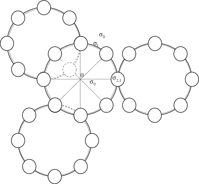
where (see figure 2)

σ1\displaystyle\sigma_{1} =\displaystyle= {𝐤∈Γ; ||𝐤|2−1|2<δ2 and |𝐤−𝐤j|>δ1=3​δ,j∈{1,2q}},\displaystyle\{\mathbf{k}\in\Gamma;\text{ }||\mathbf{k}|^{2}-1|^{2}<\delta^{2}\text{ and }|\mathbf{k}-\mathbf{k}_{j}|>\delta_{1}=\sqrt{3\delta},j\in\{1,2q\}\},
σ2,j\displaystyle\sigma_{2,j} =\displaystyle= {𝐤∈Γ; |𝐤−𝐤j|≤δ1}, σ2=∪j=12​qσ2,j.\displaystyle\{\mathbf{k}\in\Gamma;\text{ }|\mathbf{k}-\mathbf{k}_{j}|\leq\delta_{1}\},\text{ }\sigma_{2}=\cup_{j=1}^{2q}\sigma_{2,j}.
Refer to caption
Figure 2: Division of the Fourier spectrum into σ0\sigma_{0}, σ1\sigma_{1} and σ2\sigma_{2}.

In figure 2 the annulus centered at the unit circle has a thickness 2​δ2\delta and the little discs should have a radius δ1=3​δ\delta_{1}=\sqrt{3\delta}, such that the intersection of the shaded area with the shifted one, centered at the point (2𝐤1\mathbf{k}_{1},0) is, for δ\delta small enough, reduced to the disc centered at 𝐤1.\mathbf{k}_{1}. In the sequel, we choose δ=C​ϵ1/2\delta=C\epsilon^{1/2} with CC large enough and

δ1=ϵ1/4​3​C\delta_{1}=\epsilon^{1/4}\sqrt{3C}

hence 2​δ+δ2<δ122\delta+\delta^{2}<\delta_{1}^{2} is verified for ϵ1/2<1/C\epsilon^{1/2}<1/C and the intersection σ1∩{σ1+2​𝐤1}\sigma_{1}\cap\{\sigma_{1}+2\mathbf{k}_{1}\} is empty (hint: solve δ12=(1+δ)2−1\delta_{1}^{2}=(1+\delta)^{2}-1 for intersecting the circle centered in 0,0, of radius 1+δ1+\delta with the line of abscissa 11 parallel to yy axis).

This leads to (see figure 3)

σ1∩{σ1+𝐤j+𝐤l, j,l=1,..2q, 𝐤j+𝐤l≠0}=∅.\sigma_{1}\cap\{\sigma_{1}+\mathbf{k}_{j}+\mathbf{k}_{l},\text{ }j,l=1,..2q,\text{ \ }\mathbf{k}_{j}+\mathbf{k}_{l}\neq 0\}=\mathchar 1343\relax.
Refer to caption
Figure 3: Empty intersections of σ1\sigma_{1} with σ1\sigma_{1} shifted by 𝐤j+𝐤l\mathbf{k}_{j}+\mathbf{k}_{l}

The subspaces ElE_{l} are closed as intersections of closed subspaces (kernel of certain coefficients, still continuous functionnals here) and we have the orthogonal decomposition

ℋs=E0​⊕⊥​E1​⊕⊥​E2.{\mathcal{H}}_{s}=E_{0}\overset{\bot}{\oplus}E_{1}\overset{\bot}{\oplus}E_{2}.

The orthogonal projections associated with this decomposition are denoted by P0,P1,P2.P_{0},P_{1},P_{2}. We also notice that the multiplication operator by a function having a finite Fourier expansion with wave vectors in Γ\Gamma is a bounded linear operator in ℋr{\mathcal{H}}_{r} for any r≥0r\geq 0. Indeed a finite Fourier expansion belongs to ℋs{\mathcal{H}}_{s} for any s,s, and Lemmas 5 and 6 apply.

2.5 Reduction to the subspace E2E_{2}

The aim here is to solve with respect to U∈ℋsU\in{\mathcal{H}}_{s} the equation

ℒϵ​U=f,\mathcal{L}_{\epsilon}U=f, (25)

where ℒϵ\mathcal{L}_{\epsilon} is defined in (22) and where f∈ℋsf\in{\mathcal{H}}_{s} is given.

Remark 8.

We denote by ℒ0\mathcal{L}_{0} the operator ℒ0,0=ℒ0,W=(1+Δ)2=𝔏0.\mathcal{L}_{0,0}=\mathcal{L}_{0,W}=(1+\Delta)^{2}=\mathfrak{L}_{0}. For being more explicit in formulae, we denote by Pj​ℒ0​PjP_{j}\mathcal{L}_{0}P_{j} the restriction of ℒ0\mathcal{L}_{0} to the invariant subspace Ej,j=0,1,2.E_{j},j=0,1,2.

We decompose this equation on the subspaces E0,E1,E2,E_{0},E_{1},E_{2}, which gives, after noticing that the subspaces E0,E_{0}, E1,E_{1}, E2E_{2} are invariant under ℒ0,\mathcal{L}_{0}, and that ℒ0|E1\mathcal{L}_{0}|_{E_{1}}, ℒ0|E2\mathcal{L}_{0}|_{E_{2}} are bounded operators, and Pj​ℒ0​P0=0P_{j}\mathcal{L}_{0}P_{0}=0 for j∈{1,2},j\in\{1,2\},

P0​ℒϵ​U0+P0​{(ϵ2​a+ϵ4​b+ϵ6​𝒫ϵ)​(U1+U2)}\displaystyle P_{0}\mathcal{L}_{\epsilon}U_{0}+P_{0}\{(\epsilon^{2}a+\epsilon^{4}b+\epsilon^{6}\mathcal{P}_{\epsilon})(U_{1}+U_{2})\} =\displaystyle= f0\displaystyle f_{0} (26)
P1​ℒϵ​U1+P1​{(ϵ2​a+ϵ4​b+ϵ6​𝒫ϵ)​(U0+U2)}\displaystyle P_{1}\mathcal{L}_{\epsilon}U_{1}+P_{1}\{(\epsilon^{2}a+\epsilon^{4}b+\epsilon^{6}\mathcal{P}_{\epsilon})(U_{0}+U_{2})\} =\displaystyle= f1\displaystyle f_{1} (27)
P2​ℒϵ​U2+P2​{(ϵ2​a+ϵ4​b+ϵ6​𝒫ϵ)​(U0+U1)}\displaystyle P_{2}\mathcal{L}_{\epsilon}U_{2}+P_{2}\{(\epsilon^{2}a+\epsilon^{4}b+\epsilon^{6}\mathcal{P}_{\epsilon})(U_{0}+U_{1})\} =\displaystyle= f2\displaystyle f_{2} (28)

where fj=Pjf,j=0,1,2.f_{j}=P_{j}f,j=0,1,2.

We have the following

Lemma 9.

Let fix S≥0S\geq 0 and choose ss such that 0≤s≤S.0\leq s\leq S. Then, there exists ϵ0>0,\epsilon_{0}>0, such that choosing CC large enough in the definition of δ\delta, ϵ≤ϵ0\epsilon\leq\epsilon_{0}, the equation ℒϵ​U=f\mathcal{L}_{\epsilon}U=f in ℋs\mathcal{H}_{s} reduces to

ℒϵ(2)​U2=𝒬⁡(ϵ)​f\mathcal{L}_{\epsilon}^{(2)}U_{2}=\mathcal{Q}(\epsilon)f

where U2=P2​UU_{2}=P_{2}U,

ℒϵ(2)\displaystyle\mathcal{L}_{\epsilon}^{(2)} =\displaystyle= Λϵ+ϵ4​Rϵ\displaystyle\Lambda_{\epsilon}+\epsilon^{4}R_{\epsilon}
Λϵ​U2\displaystyle\Lambda_{\epsilon}U_{2} =\displaystyle= P2​(ℒ0+ϵ2​a)​U2\displaystyle P_{2}(\mathcal{L}_{0}+\epsilon^{2}a)U_{2}
ℛϵ​U2\displaystyle\mathcal{R}_{\epsilon}U_{2} =\displaystyle= P2​{b​U2−a~​(P0​ℒ0​P0)−1​P0​(a~​U2)}+O⁡(ϵ2)​U2,\displaystyle P_{2}\{bU_{2}-\mathaccent 869{a}(P_{0}\mathcal{L}_{0}P_{0})^{-1}P_{0}(\mathaccent 869{a}U_{2})\}+O(\epsilon^{2})U_{2}, (29)

Here O⁡(ϵ2)O(\epsilon^{2}) denotes a bounded linear operator in ℋs{\cal H}_{s} which norm is bounded by c​ϵ2c{\epsilon}^{2}. The components U0:=P0​UU_{0}:=P_{0}U and U1:=P1​UU_{1}:=P_{1}U are functions of U2U_{2} and ff and satisfy the following inequalities :

‖U0‖s\displaystyle||U_{0}||_{s} ≤\displaystyle\leq c​ϵ2​‖U2‖s+cϵ​‖(P0+P1)​f‖s\displaystyle c\epsilon^{2}||U_{2}||_{s}+\frac{c}{\epsilon}||(P_{0}+P_{1})f||_{s}
‖U1‖s\displaystyle||U_{1}||_{s} ≤\displaystyle\leq c​ϵ4​‖U2‖s+cϵ2​‖(ϵ​P0+P1)​f‖s\displaystyle c\epsilon^{4}||U_{2}||_{s}+\frac{c}{\epsilon^{2}}||(\epsilon P_{0}+P_{1})f||_{s}

where a~=a−a0,\mathaccent 869{a}=a-a_{0}, for a certain c>0,c>0, only depending on s,s, and RϵR_{\epsilon} and 𝒬⁡(ϵ)\mathcal{Q}(\epsilon) are bounded linear operators in ℋs\mathcal{H}_{s}, depending smoothly on ϵ\epsilon.

We need the following Lemma

Lemma 10.

For ϵ\epsilon small enough, we have

a~U1∈E0, P1(aU2)=0, P1(bU2)=0,\mathaccent 869{a}U_{1}\in E_{0},\text{ \ }P_{1}(aU_{2})=0,\text{ }P_{1}(bU_{2})=0, (30)

where a~\mathaccent 869{a} is the oscillating part of a:a:

a~=a−a0.\mathaccent 869{a}=a-a_{0}.

Moreover, the Fourier spectra of P0​(a​U2)P_{0}(aU_{2}) and P0​(b​U2)P_{0}(bU_{2}) are at a distance of order 1 of the unit circle.

By distance of order 1 of the circle, we mean a strictly positive distance as ϵ\epsilon tends to 0, in the decomposition into subspaces EjE_{j}.

Proof.

We need to prove that i) for 𝐤∈σ1,\mathbf{k}\in\sigma_{1}, then 𝐤+𝐤𝐦∉σ1∪σ2\mathbf{k}+\mathbf{k}_{\mathbf{m}}\notin\sigma_{1}\cup\sigma_{2} for 𝐤𝐦≠0,|𝐦|=2,\mathbf{k}_{\mathbf{m}}\neq 0,|\mathbf{m}|=2, and ii) for 𝐤∈σ2,\mathbf{k}\in\sigma_{2}, then 𝐤+𝐤𝐦∉σ1\mathbf{k}+\mathbf{k}_{\mathbf{m}}\notin\sigma_{1} with |𝐦|=2|\mathbf{m}|=2 or 4.4.

For showing this, let us first observe that the intersections of the unit circle with all circles of radius 1, centered at 𝐤𝐦,\mathbf{k}_{\mathbf{m}}, with 𝐤𝐦≠0,\mathbf{k}_{\mathbf{m}}\neq 0, |𝐦|=2,|\mathbf{m}|=2, are exactly the 2​q2q points 𝐤r,\mathbf{k}_{r}, r=1,…,2​q.r=1,...,2q. Let us define the region 𝔞0\mathfrak{a}_{0} (shaded region in figure 2 (a)) defined by

𝔞0=σ1∪j∈{1,..,2q}σ2,j\mathfrak{a}_{0}=\sigma_{1}\cup_{j\in\{1,..,2q\}}\sigma_{2,j}

which is the union of the annulus σ1\sigma_{1} and the discs ∪j∈{1,..,2q}σ2,j.\cup_{j\in\{1,..,2q\}}\sigma_{2,j}. Now consider the intersection of 𝔞0\mathfrak{a}_{0} with the union of shifted analogue annuli 𝔞𝐤𝐦\mathfrak{a}_{\mathbf{k}_{\mathbf{m}}}

𝔞𝐤𝐦={𝐤+𝐤𝐦;𝐤∈𝔞0, 𝐤𝐦≠0,|𝐦|=2}\mathfrak{a}_{\mathbf{k}_{\mathbf{m}}}=\{\mathbf{k}+\mathbf{k}_{\mathbf{m}};\mathbf{k}\in\mathfrak{a}_{0},\text{ }\mathbf{k}_{\mathbf{m}}\neq 0,|\mathbf{m}|=2\}

centered at all 𝐤𝐦,\mathbf{k}_{\mathbf{m}},such that |𝐦|=2|\mathbf{m}|=2 (see figure 3). It is clear that for any given q,q, and ϵ\epsilon small enough, the little discs of radius δ1\delta_{1} are such that the intersection 𝔞0∩{∪|𝐦|=2𝔞𝐤𝐦}\mathfrak{a}_{0}\cap\{\cup_{|\mathbf{m}|=2}\mathfrak{a}_{\mathbf{k}_{\mathbf{m}}}\} is exactly the union of the little closed discs centered at each 𝐤j.\mathbf{k}_{j}. It results that for U∈E1⊕E2,U\in E_{1}\oplus E_{2}, the product a~​U\mathaccent 869{a}U for which the corresponding wave vectors belong to some 𝔞𝐤𝐦,\mathfrak{a}_{\mathbf{k}_{\mathbf{m}}}, has a zero projection on E1.E_{1}. This proves that

P1(a~U1)=0, P1(a~U2)=0,P_{1}(\mathaccent 869{a}U_{1})=0,\text{ }P_{1}(\mathaccent 869{a}U_{2})=0,

which implies

P1​(a​U2)=0.P_{1}(aU_{2})=0.

It is also clear that

𝔞0∩{𝐤+𝐤𝐦;𝐤∈σ1, 𝐤𝐦≠0,|𝐦|=2}=∅,\mathfrak{a}_{0}\cap\{\mathbf{k}+\mathbf{k}_{\mathbf{m}};\mathbf{k}\in\sigma_{1},\text{ }\mathbf{k}_{\mathbf{m}}\neq 0,|\mathbf{m}|=2\}=\mathchar 1343\relax,

which moreover implies that

P2​(a~​U1)=0,P_{2}(\mathaccent 869{a}U_{1})=0,

and (30) is proved for the part concerning a.a. Now observe that we have |𝐤j+𝐤𝐦|≠1|\mathbf{k}_{j}+\mathbf{k}_{\mathbf{m}}|\neq 1 except when 𝐤j+𝐤𝐦=𝐤r\mathbf{k}_{j}+\mathbf{k}_{\mathbf{m}}=\mathbf{k}_{r} for some r∈(1,2​q).r\in(1,2q). Since we only consider the finite number of cases |𝐦|=2|\mathbf{m}|=2 or 4,4, it is clear that in choosing ϵ\epsilon small enough (i.e. δ1\delta_{1} small enough), then for 𝐤∈σ2,\mathbf{k}\in\sigma_{2}, 𝐤+𝐤𝐦∉σ1.\mathbf{k}+\mathbf{k}_{\mathbf{m}}\notin\sigma_{1}. It results in particular that

P1​(b​U2)=0.P_{1}(bU_{2})=0.

The last assertion of Lemma 10 results from the fact that |𝐤+𝐤𝐦|≠1|\mathbf{k}+\mathbf{k}_{\mathbf{m}}|\neq 1 for the Fourier spectrum of terms ∈P0​(a​U2)\in P_{0}(aU_{2}) and P0​(b​U2),P_{0}(bU_{2}), with a distance to the unit circle equivalent to ||𝐤j+𝐤𝐦|−1|\left||\mathbf{k}_{j}+\mathbf{k}_{\mathbf{m}}|-1\right| when it is not zero.    

Proof.

of Lemma 9 : We know by construction that

‖(P0​ℒ0​P0)−1‖s≤1ϵ​C2,||(P_{0}\mathcal{L}_{0}P_{0})^{-1}||_{s}\leq\frac{1}{\epsilon C^{2}},

Hence, we have

(P0​ℒϵ​P0)−1=[1+(P0​ℒ0​P0)−1​(ϵ2​a+ϵ4​b+ϵ6​𝒫ϵ)]−1​(P0​ℒ0​P0)−1,(P_{0}\mathcal{L}_{\epsilon}P_{0})^{-1}=[1+(P_{0}\mathcal{L}_{0}P_{0})^{-1}(\epsilon^{2}a+\epsilon^{4}b+\epsilon^{6}\mathcal{P}_{\epsilon})]^{-1}(P_{0}\mathcal{L}_{0}P_{0})^{-1}, (31)

and the estimate

‖ϵ2​a+ϵ4​b+ϵ6​𝒫ϵ‖s≤c⁡(s)​ϵ2||\epsilon^{2}a+\epsilon^{4}b+\epsilon^{6}\mathcal{P}_{\epsilon}||_{s}\leq c(s)\epsilon^{2}

leads for ϵ\epsilon small enough (s≤Ss\leq S) to

(P0​ℒϵ​P0)−1\displaystyle(P_{0}\mathcal{L}_{\epsilon}P_{0})^{-1} =\displaystyle= [𝕀−(P0ℒ0P0)−1(ϵ2a+ϵ4b+ϵ6𝒫ϵ)+\displaystyle[\mathbb{I}-(P_{0}\mathcal{L}_{0}P_{0})^{-1}(\epsilon^{2}a+\epsilon^{4}b+\epsilon^{6}\mathcal{P}_{\epsilon})+
+{(P0ℒ0P0)−1(ϵ2a+ϵ4b+ϵ6𝒫ϵ)}2+O(ϵ3)](P0ℒ0P0)−1\displaystyle+\{(P_{0}\mathcal{L}_{0}P_{0})^{-1}(\epsilon^{2}a+\epsilon^{4}b+\epsilon^{6}\mathcal{P}_{\epsilon})\}^{2}+O(\epsilon^{3})](P_{0}\mathcal{L}_{0}P_{0})^{-1}

with a convergent Neumann power series in the bracket, as soon as c⁡(s)​ϵC2<1,\frac{c(s)\epsilon}{C^{2}}<1, which holds for ϵ\epsilon small enough (s≤Ss\leq S). The first consequence is

‖(P0​ℒϵ​P0)−1‖s≤1ϵ⁡(C2−c⁡(s)​ϵ).||(P_{0}\mathcal{L}_{\epsilon}P_{0})^{-1}||_{s}\leq\frac{1}{\epsilon(C^{2}-c(s)\epsilon)}.

Notice that

U0=−(P0​ℒϵ​P0)−1​P0​{(ϵ2​a+ϵ4​b+ϵ6​𝒫ϵ)​(U1+U2)}+(P0​ℒϵ​P0)−1​f0U_{0}=-(P_{0}\mathcal{L}_{\epsilon}P_{0})^{-1}P_{0}\{(\epsilon^{2}a+\epsilon^{4}b+\epsilon^{6}\mathcal{P}_{\epsilon})(U_{1}+U_{2})\}+(P_{0}\mathcal{L}_{\epsilon}P_{0})^{-1}f_{0} (32)

The last property of Lemma 10 and (31) imply that in (32) we have, for ϵ∈(0,ϵ0)\epsilon\in(0,\epsilon_{0}) and for any ss

‖(P0​ℒ0​P0)−1​P0​(a​U2)‖s\displaystyle||(P_{0}\mathcal{L}_{0}P_{0})^{-1}P_{0}(aU_{2})||_{s} ≤\displaystyle\leq d⁡(s)​‖U2‖s,\displaystyle d(s)||U_{2}||_{s},
‖(P0​ℒ0​P0)−1​P0​(b​U2)‖s\displaystyle||(P_{0}\mathcal{L}_{0}P_{0})^{-1}P_{0}(bU_{2})||_{s} ≤\displaystyle\leq d⁡(s)​‖U2‖s,\displaystyle d(s)||U_{2}||_{s},
‖(P0​ℒ0​P0)−1​a​(P0​ℒ0​P0)−1​P0​(a​U2)‖s≤d⁡(s)​‖U2‖s.||(P_{0}\mathcal{L}_{0}P_{0})^{-1}a(P_{0}\mathcal{L}_{0}P_{0})^{-1}P_{0}(aU_{2})||_{s}\leq d(s)||U_{2}||_{s}.

It results that

−(P0​ℒϵ​P0)−1​P0​{(ϵ2​a+ϵ4​b+ϵ6​𝒫ϵ)​U2}\displaystyle-(P_{0}\mathcal{L}_{\epsilon}P_{0})^{-1}P_{0}\{(\epsilon^{2}a+\epsilon^{4}b+\epsilon^{6}\mathcal{P}_{\epsilon})U_{2}\} =\displaystyle= −ϵ2​(P0​ℒ0​P0)−1​P0​(a​U2)+\displaystyle-\epsilon^{2}(P_{0}\mathcal{L}_{0}P_{0})^{-1}P_{0}(aU_{2})+
+𝒪⁡(ϵ4​‖U2‖s),\displaystyle+\mathcal{O}(\epsilon^{4}||U_{2}||_{s}),

hence

U0=Q0,1​(ϵ)​U1+Q0,2​(ϵ)​U2+(P0​ℒϵ​P0)−1​f0U_{0}=Q_{0,1}(\epsilon)U_{1}+Q_{0,2}(\epsilon)U_{2}+(P_{0}\mathcal{L}_{\epsilon}P_{0})^{-1}f_{0} (33)

with

Q0,j(ϵ)=:−(P0ℒϵP0)−1P0(ϵ2a+ϵ4b+ϵ6𝒫ϵ)Pj, j=1,2,Q_{0,j}(\epsilon)=:-(P_{0}\mathcal{L}_{\epsilon}P_{0})^{-1}P_{0}(\epsilon^{2}a+\epsilon^{4}b+\epsilon^{6}\mathcal{P}_{\epsilon})P_{j},\text{ \ }j=1,2,

and for s≤S,s\leq S, ϵ∈(0,ϵ0​(S))\epsilon\in(0,\epsilon_{0}(S)) the following estimates hold:

Q0,2​(ϵ)​U2=−ϵ2​(P0​ℒ0​P0)−1​P0​(a​U2)+ϵ4​Q0,2′​(ϵ)​U2,Q_{0,2}(\epsilon)U_{2}=-\epsilon^{2}(P_{0}\mathcal{L}_{0}P_{0})^{-1}P_{0}(aU_{2})+\epsilon^{4}Q_{0,2}^{\prime}(\epsilon)U_{2},
‖Q0,1​(ϵ)​U1‖s\displaystyle||Q_{0,1}(\epsilon)U_{1}||_{s} ≤\displaystyle\leq c⁡(s)​ϵC2−c⁡(s)​ϵ​‖U1‖s≤c1​(s)​ϵ​‖U1‖s,\displaystyle\frac{c(s)\epsilon}{C^{2}-c(s)\epsilon}||U_{1}||_{s}\leq c_{1}(s)\epsilon||U_{1}||_{s}, (34)
‖Q0,2′​(ϵ)​U2‖s\displaystyle||Q_{0,2}^{\prime}(\epsilon)U_{2}||_{s} ≤\displaystyle\leq c1​(s)​‖U2‖s,\displaystyle c_{1}(s)||U_{2}||_{s},
‖(P0​ℒϵ​P0)−1​f0‖s\displaystyle||(P_{0}\mathcal{L}_{\epsilon}P_{0})^{-1}f_{0}||_{s} ≤\displaystyle\leq c1​(s)ϵ​‖f0‖s.\displaystyle\frac{c_{1}(s)}{\epsilon}||f_{0}||_{s}.

It results from Lemma 10 that equation (27) leads to

P1​(ℒ0+ϵ2​a0+ϵ4​b+ϵ6​𝒫ϵ)​U1+P1​{(ϵ2​a+ϵ4​b+ϵ6​𝒫ϵ)​U0}+P1​ϵ6​𝒫ϵ​U2=f1P_{1}(\mathcal{L}_{0}+\epsilon^{2}a_{0}+\epsilon^{4}b+\epsilon^{6}\mathcal{P}_{\epsilon})U_{1}+P_{1}\{(\epsilon^{2}a+\epsilon^{4}b+\epsilon^{6}\mathcal{P}_{\epsilon})U_{0}\}+P_{1}\epsilon^{6}\mathcal{P}_{\epsilon}U_{2}=f_{1} (35)

and since a0=3>0a_{0}=3>0 and the operator P1​ℒ0​P1P_{1}\mathcal{L}_{0}P_{1} is positive, we can invert the operator P1​(ℒ0+ϵ2​a0)​P1P_{1}(\mathcal{L}_{0}+\epsilon^{2}a_{0})P_{1} with the estimate

‖{P1​(ℒ0+ϵ2​a0)​P1}−1‖≤13​ϵ2.||\{P_{1}(\mathcal{L}_{0}+\epsilon^{2}a_{0})P_{1}\}^{-1}||\leq\frac{1}{3\epsilon^{2}}.

Now replacing U0U_{0} by its expression (33) into equation (35), we introduce an operator acting on U1U_{1} of the form

P1​(ϵ4​b+ϵ6​𝒫ϵ)​P1+P1​(ϵ2​a+ϵ4​b+ϵ6​𝒫ϵ)​Q0,1​(ϵ)P_{1}(\epsilon^{4}b+\epsilon^{6}\mathcal{P}_{\epsilon})P_{1}+P_{1}(\epsilon^{2}a+\epsilon^{4}b+\epsilon^{6}\mathcal{P}_{\epsilon})Q_{0,1}(\epsilon)

which is bounded by O⁡(ϵ3),O(\epsilon^{3}), perturbing P1​(ℒ0+ϵ2​a0)​P1P_{1}(\mathcal{L}_{0}+\epsilon^{2}a_{0})P_{1} the inverse of which is bounded by 1/3​ϵ21/3\epsilon^{2}. It results that, for ϵ\epsilon small enough, the operator acting on U1U_{1} has a bounded inverse, with

‖{P1​[ℒϵ+(ϵ2​a+ϵ4​b+ϵ6​𝒫ϵ)​Q0,1​(ϵ)]​P1}−1‖s≤1ϵ2.||\{P_{1}[\mathcal{L}_{\epsilon}+(\epsilon^{2}a+\epsilon^{4}b+\epsilon^{6}\mathcal{P}_{\epsilon})Q_{0,1}(\epsilon)]P_{1}\}^{-1}||_{s}\leq\frac{1}{\epsilon^{2}}.

Moreover by Lemma 10 we have P1​[a​(P0​ℒ0​P0)−1​P0​(a​U2)]=0,P_{1}[a(P_{0}\mathcal{L}_{0}P_{0})^{-1}P_{0}(aU_{2})]=0, hence it results that there are bounded linear operators

ℬϵ(0):E2→E0, ℬϵ(1):E2→E1,\mathcal{B}_{\epsilon}^{(0)}:E_{2}\rightarrow E_{0},\text{ \ }\mathcal{B}_{\epsilon}^{(1)}:E_{2}\rightarrow E_{1},

such that

U1\displaystyle U_{1} =\displaystyle= ϵ4​ℬ(1)​(ϵ)​U2+1ϵ​𝒬(1,0)​(ϵ)​f0+1ϵ2​𝒬(1,1)​(ϵ)​f1,\displaystyle\epsilon^{4}\mathcal{B}^{(1)}(\epsilon)U_{2}+\frac{1}{\epsilon}\mathcal{Q}^{(1,0)}\mathcal{(}\epsilon)f_{0}+\frac{1}{\epsilon^{2}}\mathcal{Q}^{(1,1)}\mathcal{(}\epsilon)f_{1}, (36)
U0\displaystyle U_{0} =\displaystyle= ϵ2​ℬ(0)​(ϵ)​U2+1ϵ​𝒬(0,0)​(ϵ)​f0+1ϵ​𝒬(0,1)​(ϵ)​f1,\displaystyle\epsilon^{2}\mathcal{B}^{(0)}(\epsilon)U_{2}+\frac{1}{\epsilon}\mathcal{Q}^{(0,0)}\mathcal{(}\epsilon)f_{0}+\frac{1}{\epsilon}\mathcal{Q}^{(0,1)}\mathcal{(}\epsilon)f_{1}, (37)

with the estimates

‖ℬ(j)​(ϵ)‖s\displaystyle||\mathcal{B}^{(j)}(\epsilon)||_{s} ≤\displaystyle\leq c2​(s),j=0,1,\displaystyle c_{2}(s),j=0,1,
‖𝒬(i,j)​(ϵ)‖s\displaystyle||\mathcal{Q}^{(i,j)}\mathcal{(}\epsilon)||_{s} ≤\displaystyle\leq c2(s), i,j=0,1,\displaystyle c_{2}(s),\text{ \ }i,j=0,1,

uniform in ϵ∈(0,ϵ0)\epsilon\in(0,\epsilon_{0}) and in WW bounded in ℋs.\mathcal{H}_{s}. Moreover, as ϵ→0\epsilon\rightarrow 0

ℬ(0)​(ϵ)\displaystyle\mathcal{B}^{(0)}(\epsilon) =\displaystyle= ℬ0(0)+𝒪⁡(ϵ2),\displaystyle\mathcal{B}_{0}^{(0)}+\mathcal{O}(\epsilon^{2}),
ℬ0(0)​U2\displaystyle\mathcal{B}_{0}^{(0)}U_{2} ∼\displaystyle\sim −(P0​ℒ0​P0)−1​P0​(a~​U2).\displaystyle-(P_{0}\mathcal{L}_{0}P_{0})^{-1}P_{0}(\mathaccent 869{a}U_{2}).

Equation (28) now reads

P2​ℒϵ​U2+P2​{(ϵ2​a+ϵ4​b+ϵ6​𝒫ϵ)​U0}+P2​{(ϵ4​b+ϵ6​𝒫ϵ)​U1}=f2P_{2}\mathcal{L}_{\epsilon}U_{2}+P_{2}\{(\epsilon^{2}a+\epsilon^{4}b+\epsilon^{6}\mathcal{P}_{\epsilon})U_{0}\}+P_{2}\{(\epsilon^{4}b+\epsilon^{6}\mathcal{P}_{\epsilon})U_{1}\}=f_{2}

and replacing U0U_{0} and U1U_{1} by their expressions (37), (36) in function of U2U_{2} leads to

P2ℒϵU2+P2{(ϵ2a+ϵ4b+ϵ6𝒫ϵ)ϵ2ℬ(0)(ϵ)U2+\displaystyle P_{2}\mathcal{L}_{\epsilon}U_{2}+P_{2}\{(\epsilon^{2}a+\epsilon^{4}b+\epsilon^{6}\mathcal{P}_{\epsilon})\epsilon^{2}\mathcal{B}^{(0)}(\epsilon)U_{2}+
+P2​{(ϵ4​b+ϵ6​𝒫ϵ)​ϵ4​ℬ(1)​(ϵ)​U2}\displaystyle+P_{2}\{(\epsilon^{4}b+\epsilon^{6}\mathcal{P}_{\epsilon})\epsilon^{4}\mathcal{B}^{(1)}(\epsilon)U_{2}\}
=\displaystyle= f2−P2​((ϵ2​a+ϵ4​b+ϵ6​𝒫ϵ)​[1ϵ​𝒬(0,0)​(ϵ)​f0+1ϵ​𝒬(0,1)​(ϵ)​f1])+\displaystyle f_{2}-P_{2}\left((\epsilon^{2}a+\epsilon^{4}b+\epsilon^{6}\mathcal{P}_{\epsilon})[\frac{1}{\epsilon}\mathcal{Q}^{(0,0)}\mathcal{(}\epsilon)f_{0}+\frac{1}{\epsilon}\mathcal{Q}^{(0,1)}\mathcal{(}\epsilon)f_{1}]\right)+
−P2​((ϵ4​b+ϵ6​𝒫ϵ)​[1ϵ​𝒬(1,0)​(ϵ)​f0+1ϵ2​𝒬(1,1)​(ϵ)​f1]),\displaystyle-P_{2}\left((\epsilon^{4}b+\epsilon^{6}\mathcal{P}_{\epsilon})[\frac{1}{\epsilon}\mathcal{Q}^{(1,0)}\mathcal{(}\epsilon)f_{0}+\frac{1}{\epsilon^{2}}\mathcal{Q}^{(1,1)}\mathcal{(}\epsilon)f_{1}]\right),

this gives (see the definition of Λϵ\Lambda_{\epsilon} in Lemma 9)

Λϵ​U2+ϵ4​Rϵ​U2=𝒬⁡(ϵ)​f\Lambda_{\epsilon}U_{2}+\epsilon^{4}R_{\epsilon}U_{2}=\mathcal{Q}(\epsilon)f

with the announced properties for bounded operators RϵR_{\epsilon} and 𝒬⁡(ϵ)\mathcal{Q}(\epsilon) in ℋs.\mathcal{H}_{s}. Lemma 9 is proved.    

2.6 Structure of the reduced operator Λϵ\Lambda_{\epsilon}

2.6.1 General structure - Invariant subspaces

We study in this section the structure of the operator Λϵ\Lambda_{\epsilon} defined by (29). We first observe that we deal with functions UU which are invariant under the rotation RπqR_{\frac{\pi}{q}} of the plane. So, let us define a new subspace of ℋs\mathcal{H}_{s} for such functions:

E2(S)={U∈E2;U⁡(Rπq​𝐱)=U⁡(𝐱)}.E_{2}^{(S)}=\{U\in E_{2};U(R_{\frac{\pi}{q}}\mathbf{x})=U(\mathbf{x})\}.

This implies immediately that

U(𝐤)=U(Rπq​𝐤),U^{(\mathbf{k})}=U^{(R_{\frac{\pi}{q}}\mathbf{k})}, (38)

and for any U∈E2(S)U\in E_{2}^{(S)} we have the following decomposition

U=∑j=1,…,2​qU2,jU=\sum_{j=1,...,2q}U_{2,j}

where

U2,j​(𝐱)=∑𝐤∈σ2,jU(𝐤)​ei​𝐤⋅𝐱=U2,1​(R(1−j)​πq​𝐱).U_{2,j}(\mathbf{x})=\sum_{\mathbf{k}\in\sigma_{2,j}}U^{(\mathbf{k})}e^{i\mathbf{k}\cdot\mathbf{x}}=U_{2,1}(R_{\frac{(1-j)\pi}{q}}\mathbf{x}). (39)

It results that any U∈E2(S)U\in E_{2}^{(S)} may be written as

U⁡(𝐱)=∑j=1,…,2​qU2,1​(R(1−j)​πq​𝐱).U(\mathbf{x})=\sum_{j=1,...,2q}U_{2,1}(R_{\frac{(1-j)\pi}{q}}\mathbf{x}).

Let us notice that in the little disc σ2,1\sigma_{2,1} we have

σ2,1∋𝐤=𝐤1+𝐤′,|𝐤′|≤δ1=ϵ1/4​3​C,\sigma_{2,1}\ni\mathbf{k}=\mathbf{k}_{1}+\mathbf{k}^{\prime},|\mathbf{k}^{\prime}|\leq\delta_{1}=\epsilon^{1/4}\sqrt{3C},

and let decompose the discs σ2,l\sigma_{2,l} into 2​q2q equal sectors 𝐤l+Σm,m=1,…,2​q\mathbf{k}_{l}+\Sigma_{m},m=1,...,2q such that

Σm={𝐤′∈Γ;|𝐤′|≤δ1,arg𝐤′∈[(m−1)​πq−π2​q,(m−1)​πq+π2​q)}.\Sigma_{m}=\left\{\mathbf{k}^{\prime}\in\Gamma;|\mathbf{k}^{\prime}|\leq\delta_{1},\arg\mathbf{k}^{\prime}\in[\frac{(m-1)\pi}{q}-\frac{\pi}{2q},\frac{(m-1)\pi}{q}+\frac{\pi}{2q})\right\}. (40)

For any 𝐤′∈Σl\mathbf{k}^{\prime}\in\Sigma_{l}, we define the set of 2​q2q spectral points σ𝐤′(l)\sigma_{\mathbf{k}^{\prime}}^{(l)} by

σ𝐤′(l)={𝐤=𝐤j+𝐤′∈σ2,j; j=1,…,2q}.\sigma_{\mathbf{k}^{\prime}}^{(l)}=\left\{\mathbf{k}=\mathbf{k}_{j}+\mathbf{k}^{\prime}\in\sigma_{2,j};\text{ }j=1,...,2q\right\}.

The subspace of ℋs\mathcal{H}_{s} associated with σ𝐤′(l)\sigma_{\mathbf{k}^{\prime}}^{(l)} is denoted by E2,𝐤′(l),E_{2,\mathbf{k}^{\prime}}^{(l)}, so that any U∈E2(S)U\in E_{2}^{(S)} may be written as

U⁡(𝐱)\displaystyle U(\mathbf{x}) =\displaystyle= ∑j=1,…,2​q∑𝐤1+𝐤′∈σ2,1U(𝐤1+𝐤′)​ei⁡(𝐤j+R(j−1)​πq​𝐤′)⋅𝐱\displaystyle\sum_{j=1,...,2q}\sum_{\mathbf{k}_{1}+\mathbf{k}^{\prime}\in\sigma_{2,1}}U^{(\mathbf{k}_{1}+\mathbf{k}^{\prime})}e^{i(\mathbf{k}_{j}+R_{\frac{(j-1)\pi}{q}}\mathbf{k}^{\prime})\cdot\mathbf{x}}
=\displaystyle= ∑l=1,…,2​q∑𝐤′∈Σl∑j=1,…,2​qU(𝐤1+R(1−j)​πq​𝐤′)​ei⁡(𝐤j+𝐤′)⋅𝐱,\displaystyle\sum_{l=1,...,2q}\sum_{\mathbf{k}^{\prime}\in\Sigma_{l}}\sum_{j=1,...,2q}U^{(\mathbf{k}_{1}+R_{\frac{(1-j)\pi}{q}}\mathbf{k}^{\prime})}e^{i(\mathbf{k}_{j}+\mathbf{k}^{\prime})\cdot\mathbf{x}},

hence

U\displaystyle U =\displaystyle= ∑l=12​q∑𝐤′∈ΣlU(l,𝐤′), U(l,𝐤′)∈E2,𝐤′(l),\displaystyle\sum_{l=1}^{2q}\sum_{\mathbf{k}^{\prime}\in\Sigma_{l}}U^{(l,\mathbf{k}^{\prime})},\text{ \ }U^{(l,\mathbf{k}^{\prime})}\in E_{2,\mathbf{k}^{\prime}}^{(l)},
U(l,𝐤′)​(𝐱)\displaystyle U^{(l,\mathbf{k}^{\prime})}(\mathbf{x}) =\displaystyle= ∑j=1,…,2​qU(𝐤1+R(1−j)​πq​𝐤′)​ei⁡(𝐤j+𝐤′)⋅𝐱=∑j=1,…,2​qU(𝐤j+𝐤′)​ei⁡(𝐤j+𝐤′)⋅𝐱\displaystyle\sum_{j=1,...,2q}U^{(\mathbf{k}_{1}+R_{\frac{(1-j)\pi}{q}}\mathbf{k}^{\prime})}e^{i(\mathbf{k}_{j}+\mathbf{k}^{\prime})\cdot\mathbf{x}}=\sum_{j=1,...,2q}U^{(\mathbf{k}_{j}+\mathbf{k}^{\prime})}e^{i(\mathbf{k}_{j}+\mathbf{k}^{\prime})\cdot\mathbf{x}}

and any U∈E2(S)U\in E_{2}^{(S)} is completely determined by the set of 2​q−2q- dimensional U(1,𝐤′)∈E2,𝐤′(1),U^{(1,\mathbf{k}^{\prime})}\in E_{2,\mathbf{k}^{\prime}}^{(1)}, 𝐤′∈Σ1,\mathbf{k}^{\prime}\in\Sigma_{1}, identified with the set of components

{U(𝐤j+𝐤′)=U(𝐤1+R(1−j)​πq​𝐤′), j=1,…,2q}.\{U^{(\mathbf{k}_{j}+\mathbf{k}^{\prime})}=U^{(\mathbf{k}_{1}+R_{\frac{(1-j)\pi}{q}}\mathbf{k}^{\prime})},\text{ \ }j=1,...,2q\}.

Indeed we have

U(l,𝐤′)​(𝐱)=U(l+1,Rπq​𝐤′)​(Rπq​𝐱),U^{(l,\mathbf{k}^{\prime})}(\mathbf{x})=U^{(l+1,R_{\frac{\pi}{q}}\mathbf{k}^{\prime})}(R_{\frac{\pi}{q}}\mathbf{x}),

hence

U(l,𝐤′)​(𝐱)\displaystyle U^{(l,\mathbf{k}^{\prime})}(\mathbf{x}) =\displaystyle= U(1,R(1−l)​πq​𝐤′)(R(1−l)​πq𝐱), 𝐤′∈Σl,\displaystyle U^{(1,R_{(1-l)\frac{\pi}{q}}\mathbf{k}^{\prime})}(R_{(1-l)\frac{\pi}{q}}\mathbf{x}),\text{ \ }\mathbf{k}^{\prime}\in\Sigma_{l},
U(l,R(l−1)​πq​𝐤′)​(𝐱)\displaystyle U^{(l,R_{\frac{(l-1)\pi}{q}}\mathbf{k}^{\prime})}(\mathbf{x}) =\displaystyle= ∑j=1,…,2​qU(𝐤1+R(l−j)​πq​𝐤′)ei⁡(𝐤j+R(l−1)​πq​𝐤′)⋅𝐱, 𝐤′∈Σ1,\displaystyle\sum_{j=1,...,2q}U^{({\mathbf{k}_{1}+R_{\frac{(l-j)\pi}{q}}\mathbf{k}^{\prime}})}e^{i(\mathbf{k}_{j}+R_{\frac{(l-1)\pi}{q}}\mathbf{k}^{\prime})\cdot\mathbf{x}},\text{ \ }\mathbf{k}^{\prime}\in\Sigma_{1},

where

U(1,𝐤′)(𝐱)=∑j=1,…,2​qU(𝐤1+R(1−j)​πq​𝐤′)ei⁡(𝐤j+𝐤′)⋅𝐱, 𝐤′∈Σ1,U^{(1,\mathbf{k}^{\prime})}(\mathbf{x})=\sum_{j=1,...,2q}U^{({\mathbf{k}_{1}+R_{\frac{(1-j)\pi}{q}}\mathbf{k}^{\prime}})}e^{i(\mathbf{k}_{j}+\mathbf{k}^{\prime})\cdot\mathbf{x}},\text{ \ }\mathbf{k}^{\prime}\in\Sigma_{1}, (41)

and we observe that the coordinates of U(l,R(l−1)​πq​𝐤′),𝐤′∈Σ1,U^{(l,R_{\frac{(l-1)\pi}{q}}\mathbf{k}^{\prime})},\mathbf{k}^{\prime}\in\Sigma_{1}, correspond to those shifted of U(1,𝐤′)U^{(1,\mathbf{k}^{\prime})}. Moreover we have

U⁡(𝐱)=∑l=12​q∑𝐤′∈Σ1U(1,𝐤′)​(R(1−l)​πq​𝐱).U(\mathbf{x})=\sum_{l=1}^{2q}\sum_{\mathbf{k}^{\prime}\in\Sigma_{1}}U^{(1,\mathbf{k}^{\prime})}(R_{(1-l)\frac{\pi}{q}}\mathbf{x}). (42)

From now on, we denote by E2,𝐤′E_{2,\mathbf{k}^{\prime}} the previously defined 2q-dimensional subspace E2,𝐤′(1)E_{2,\mathbf{k}^{\prime}}^{(1)}.

Looking at the form of the operator Λϵ\Lambda_{\epsilon} we see that the wave vector 𝐤\mathbf{k} of UU is shifted by 𝐤𝐦,|𝐦|=2\mathbf{k}_{\mathbf{m}},|\mathbf{m}|=2 at order ϵ2,\epsilon^{2}, and |𝐦|=4|\mathbf{m}|=4 at order ϵ4.\epsilon^{4}. Now, we observe that for a fixed finite |𝐦||\mathbf{m}|, if the combination

𝐤𝐦−(𝐤1−𝐤j)\mathbf{k}_{\mathbf{m}}-(\mathbf{k}_{1}-\mathbf{k}_{j})

is not 0, then it has a minimal length of order 1 as ϵ\epsilon tends to 00. It results that for 𝐤=𝐤1+𝐤′∈σ2,1,\mathbf{k}=\mathbf{k}_{1}+\mathbf{k}^{\prime}\in\sigma_{2,1}, and 𝐥=𝐤j+𝐥′∈σ2,j\mathbf{l}=\mathbf{k}_{j}+\mathbf{l}^{\prime}\in\sigma_{2,j} with

𝐤𝐦−(𝐤−𝐥)≠0\mathbf{k}_{\mathbf{m}}-(\mathbf{k}-\mathbf{l})\neq 0

then, for ϵ\epsilon small enough

𝐤𝐦−(𝐤−𝐥)=𝒪⁡(1).\mathbf{k}_{\mathbf{m}}-(\mathbf{k}-\mathbf{l})=\mathcal{O}(1).

It results that the only possibility for going from 𝐥∈σ2,j\mathbf{l}\in\sigma_{2,j} to σ2,1\sigma_{2,1} is to add 𝐤𝐦=𝐤1+𝐤j+q=𝐤1−𝐤j\mathbf{k}_{\mathbf{m}}=\mathbf{k}_{1}+\mathbf{k}_{j+q}=\mathbf{k}_{1}-\mathbf{k}_{j}. It results that the system

𝐤𝐦+𝐥=𝐤, 𝐥=𝐤j+𝐥′, 𝐤=𝐤j+𝐤′\mathbf{k}_{\mathbf{m}}+\mathbf{l=k},\text{ }\mathbf{l}=\mathbf{k}_{j}+\mathbf{l}^{\prime},\text{ }\mathbf{k}=\mathbf{k}_{j}+\mathbf{k}^{\prime}

has the only solution

𝐥′=𝐤′.\mathbf{l}^{\prime}=\mathbf{k}^{\prime}. (43)

It should be clear that 𝐤𝐦\mathbf{k}_{\mathbf{m}} comes from terms with many possible combinations, not only trivial ones as for q=4.q=4. For example for q=6,q=6, the terms occuring in the coefficients giving 𝐤𝐦\mathbf{k}_{\mathbf{m}} are even more frequent at order ϵ4\epsilon^{4} because of the existing special combinations 𝐤j+Rπ/3​𝐤j+R2​π/3​𝐤j=0.\mathbf{k}_{j}+R_{\pi/3}\mathbf{k}_{j}+R_{2\pi/3}\mathbf{k}_{j}=0. However, in all cases we can write, for 𝐤=𝐤1+𝐤′∈σ2,1\mathbf{k}=\mathbf{k}_{1}+\mathbf{k}^{\prime}\in\sigma_{2,1}

(Λϵ​U)(𝐤1+𝐤′)=∑j=1Qγj​(𝐤,ϵ)​U(𝐤j+𝐤′).(\Lambda_{\epsilon}U)^{(\mathbf{k}_{1}+\mathbf{k}^{\prime})}=\sum_{j=1}^{Q}\gamma_{j}(\mathbf{k},\epsilon)U^{(\mathbf{k}_{j}+\mathbf{k}^{\prime})}. (44)
Remark 11.

The argument ϵ\epsilon in γj​(𝐤,ϵ)\gamma_{j}(\mathbf{k},\epsilon) only refers to the perturbation of P2​ℒ0​P2P_{2}\mathcal{L}_{0}P_{2} in Λϵ\Lambda_{\epsilon} (see (29)), and not on the fact that P2P_{2} also depends on ϵ\epsilon via the radii of the little discs composing the set σ2\sigma_{2} which are O⁡(ϵ1/4)O(\epsilon^{1/4}).

Remark 12.

Due to the form of orders ϵ2\epsilon^{2} and ϵ4\epsilon^{4} in Λϵ\Lambda_{\epsilon} and ℒϵ(2)\mathcal{L}_{\epsilon}^{(2)}, and because of (43), we notice that the dependency in 𝐤\mathbf{k} of the coefficients γj​(𝐤,ϵ)\gamma_{j}(\mathbf{k},\epsilon) only occurs at orders ϵ0\epsilon^{0} and ϵ4\epsilon^{4}. Indeed, the dependency in 𝐤\mathbf{k} comes from operators ℒ0\mathcal{L}_{0} at order 0 and (P0​ℒ0​P0)−1(P_{0}\mathcal{L}_{0}P_{0})^{-1} in the term P2​{a~​(P0​ℒ0​P0)−1​P0​(a~​U)}P_{2}\{\mathaccent 869{a}(P_{0}\mathcal{L}_{0}P_{0})^{-1}P_{0}(\mathaccent 869{a}U)\} at order ϵ4.\epsilon^{4}.

The property that Λϵ​U\Lambda_{\epsilon}U is invariant under the rotation RπqR_{\frac{\pi}{q}} and the identity

R−πq​𝐤~+𝐤j−𝐤1=R−πq​(𝐤~+𝐤j+1−𝐤2)R_{\frac{-\pi}{q}}\mathaccent 869{\mathbf{k}}+\mathbf{k}_{j}-\mathbf{k}_{1}=R_{\frac{-\pi}{q}}(\mathaccent 869{\mathbf{k}}+\mathbf{k}_{j+1}-\mathbf{k}_{2})

lead to

(ΛϵU)(𝐤~)=∑j=12​qγj(R−πq𝐤~,ϵ)U(𝐤~+𝐤j+1−𝐤2), 𝐤~=Rπq𝐤∈σ2,2.(\Lambda_{\epsilon}U)^{(\mathaccent 869{\mathbf{k}})}=\sum_{j=1}^{2q}\gamma_{j}(R_{\frac{-\pi}{q}}\mathaccent 869{\mathbf{k}},\epsilon)U^{(\mathaccent 869{\mathbf{k}}+\mathbf{k}_{j+1}-\mathbf{k}_{2})},\text{ }\mathaccent 869{\mathbf{k}}=R_{\frac{\pi}{q}}\mathbf{k}\in\sigma_{2,2}.

Choosing σ2,2∋𝐤~=𝐤′+𝐤2,\sigma_{2,2}\ni\mathaccent 869{\mathbf{k}}=\mathbf{k}^{\prime}+\mathbf{k}_{2}, |𝐤′|≤δ1,\mathbf{|k}^{\prime}|\leq\delta_{1}, we then have

(Λϵ​U)(𝐤′+𝐤2)=∑j=12​qγj​(R−πq​𝐤′+𝐤1,ϵ)​U(𝐤′+𝐤j+1).(\Lambda_{\epsilon}U)^{(\mathbf{k}^{\prime}+\mathbf{k}_{2})}=\sum_{j=1}^{2q}\gamma_{j}(R_{\frac{-\pi}{q}}\mathbf{k}^{\prime}+\mathbf{k}_{1},\epsilon)U^{(\mathbf{k}^{\prime}+\mathbf{k}_{j+1})}. (45)

In the same way, after identifying j+2​qj+2q with j,j, we obtain for r=1,…,2​qr=1,...,2q

(Λϵ​U)(𝐤′+𝐤r)\displaystyle(\Lambda_{\epsilon}U)^{(\mathbf{k}^{\prime}+\mathbf{k}_{r})} =\displaystyle= ∑j=12​qγj​(Rπ⁡(1−r)q​𝐤′+𝐤1,ϵ)​U(𝐤′+𝐤j+r−1),\displaystyle\sum_{j=1}^{2q}\gamma_{j}\left(R_{\frac{\pi(1-r)}{q}}\mathbf{k}^{\prime}+\mathbf{k}_{1},\epsilon\right)U^{(\mathbf{k}^{\prime}+\mathbf{k}_{j+r-1})},
=\displaystyle= ∑j=12​qγj+1−r​(Rπ⁡(1−r)q​𝐤′+𝐤1,ϵ)​U(𝐤′+𝐤j).\displaystyle\sum_{j=1}^{2q}\gamma_{j+1-r}\left(R_{\frac{\pi(1-r)}{q}}\mathbf{k}^{\prime}+\mathbf{k}_{1},\epsilon\right)U^{(\mathbf{k}^{\prime}+\mathbf{k}_{j})}.

The important result is that, for a fixed 𝐤=𝐤1+𝐤′,𝐤′∈Σ1,\mathbf{k}=\mathbf{k}_{1}+\mathbf{k}^{\prime},\mathbf{k}^{\prime}\in\Sigma_{1}, the subspace E2,𝐤′E_{2,\mathbf{k}^{\prime}} is invariant under the operator Λϵ\Lambda_{\epsilon} then denoted Λϵ(𝐤′).\Lambda_{\epsilon}^{(\mathbf{k}^{\prime})}. Hence the 2​q×2​q2q\times 2q matrices of Λϵ(𝐤′)\Lambda_{\epsilon}^{(\mathbf{k}^{\prime})} are uncoupled for different 𝐤′∈Σ1.\mathbf{k}^{\prime}\in\Sigma_{1}. We notice that if γj\gamma_{j} were independent of 𝐤,\mathbf{k}, the lines of the matrix of Λϵ(𝐤′)\Lambda_{\epsilon}^{(\mathbf{k}^{\prime})} would be deduced each from the previous one by a simple right shift.

The next useful property of Λϵ\Lambda_{\epsilon} is its self-adjointness in E2E_{2} with the Hilbert structure of ℋ0\mathcal{H}_{0}. This property is immediate from the definition (29) with the scalar product of the space ℋs\mathcal{H}_{s} for s=0.s=0. It should be noticed that the full linear operator ℒϵ,W(2)\mathcal{L}_{\epsilon,W}^{(2)} acting in E2E_{2} is not selfadjoint in general. Now, isolating the coordinates U(𝐤′+𝐤j),U^{(\mathbf{k}^{\prime}+\mathbf{k}_{j})}, j=1,…,2​qj=1,...,2q for 𝐤′∈Σ1,\mathbf{k}^{\prime}\in\Sigma_{1}, we still have, for any fixed 𝐤′\mathbf{k}^{\prime}, a 2​q×2​q2q\times 2q self-adjoint matrix Λϵ(𝐤′)\Lambda_{\epsilon}^{(\mathbf{k}^{\prime})} due to the previous self-adjointness of the operator Λϵ\Lambda_{\epsilon} in ℋ0.\mathcal{H}_{0}. It results that we have

γj+1−r​(Rπ⁡(1−r)q​𝐤′+𝐤1,ϵ)=γr+1−j​(Rπ⁡(1−j)q​𝐤′+𝐤1,ϵ).\gamma_{j+1-r}\left(R_{\frac{\pi(1-r)}{q}}\mathbf{k}^{\prime}+\mathbf{k}_{1},\epsilon\right)=\gamma_{r+1-j}\left(R_{\frac{\pi(1-j)}{q}}\mathbf{k}^{\prime}+\mathbf{k}_{1},\epsilon\right). (46)

We sum up these results in the following

Lemma 13.

The subspace E2(S)E_{2}^{(S)} of ℋs\mathcal{H}_{s} consisting of functions invariant under rotations by π/q\pi/q may be decomposed into the following Hilbert sum

E2(S)=⊕𝐤′∈Σ1⊥​E2,𝐤′E_{2}^{(S)}=\underset{\mathbf{k}^{\prime}\in\Sigma_{1}}{\overset{\bot}{\oplus}}E_{2,\mathbf{k}^{\prime}}

where we identify the wave vector 𝐤\mathbf{k} with Rπq​𝐤R_{\frac{\pi}{q}}\mathbf{k} i.e., 𝐤1+𝐤′∈σ2,1\mathbf{k}_{1}+\mathbf{k}^{\prime}\in\sigma_{2,1} with 𝐤j+Rπ⁡(j−1)q​𝐤′∈σ2,j\mathbf{k}_{j}+R_{\frac{\pi(j-1)}{q}}\mathbf{k}^{\prime}\in\sigma_{2,j} (see (42)).

The 2​q−2q- dimensional subspace E2,𝐤′E_{2,\mathbf{k}^{\prime}} is invariant under the operator Λϵ.\Lambda_{\epsilon}. Defining the coefficients γj​(𝐤,ϵ)\gamma_{j}(\mathbf{k},\epsilon) by

(ΛϵU)(𝐤′+𝐤1)=∑j=12​qγj(𝐤,ϵ)U(𝐤′+𝐤j), 𝐤∈σ2,1(\Lambda_{\epsilon}U)^{(\mathbf{k}^{\prime}+\mathbf{k}_{1})}=\sum_{j=1}^{2q}\gamma_{j}(\mathbf{k},\epsilon)U^{(\mathbf{k}^{\prime}+\mathbf{k}_{j})},\text{ }\mathbf{k}\in\sigma_{2,1}

the 2​q×2​q2q\times 2q matrix of the restriction Λϵ(𝐤′)\Lambda_{\epsilon}^{(\mathbf{k}^{\prime})} of Λϵ\Lambda_{\epsilon} to E2,𝐤′E_{2,\mathbf{k}^{\prime}} is symmetric and satisfies

γj+1−r​(Rπ⁡(1−r)q​𝐤′+𝐤1,ϵ)=γr+1−j​(Rπ⁡(1−j)q​𝐤′+𝐤1,ϵ)\gamma_{j+1-r}\left(R_{\frac{\pi(1-r)}{q}}\mathbf{k}^{\prime}+\mathbf{k}_{1},\epsilon\right)=\gamma_{r+1-j}\left(R_{\frac{\pi(1-j)}{q}}\mathbf{k}^{\prime}+\mathbf{k}_{1},\epsilon\right)

for any 𝐤′∈Σ1.\mathbf{k}^{\prime}\in\Sigma_{1}.

Let us define Λ0(𝐤′)\Lambda_{0}^{({\mathbf{k}}^{\prime})} which is a diagonal matrix with

γ1(𝐤,0)=(|𝐤|2−1)2,γ2(𝐤,0)=0,….γ2​q(𝐤,0)=0.\gamma_{1}(\mathbf{k},0)=(|\mathbf{k}|^{2}-1)^{2},\gamma_{2}(\mathbf{k},0)=0,....\gamma_{2q}(\mathbf{k},0)=0.

For 𝐤=𝐤′+𝐤j∈σ2,j,\mathbf{k}=\mathbf{k}^{\prime}+\mathbf{k}_{j}\in\sigma_{2,j}, we define

βj(𝐤′)=(|𝐤′+𝐤j|2−1)2,j=1,…,2q.\beta_{j}(\mathbf{k}^{\prime})=(|\mathbf{k}^{\prime}+\mathbf{k}_{j}|^{2}-1)^{2},\quad j=1,...,2q. (47)

Hence for j=1,…,2​qj=1,...,2q

γ1​(Rπ⁡(1−j)q​𝐤′+𝐤1,0)\displaystyle\gamma_{1}\left(R_{\frac{\pi(1-j)}{q}}\mathbf{k}^{\prime}+\mathbf{k}_{1},0\right) =\displaystyle= (|Rπ⁡(1−j)q​𝐤′+𝐤1|2−1)2=βj​(𝐤′)\displaystyle\left(\left|R_{\frac{\pi(1-j)}{q}}\mathbf{k}^{\prime}+\mathbf{k}_{1}\right|^{2}-1\right)^{2}=\beta_{j}(\mathbf{k}^{\prime})
=\displaystyle= (2​𝐤j⋅𝐤′+|𝐤′|2)2,\displaystyle(2\mathbf{k}_{j}\cdot\mathbf{k}^{\prime}+|\mathbf{k}^{\prime}|^{2})^{2},

and Λ0(𝐤′)\Lambda_{0}^{(\mathbf{k}^{\prime})} reads

Λ0(𝐤′)=(β1​(𝐤′)0..0.000β2​(𝐤′)..0.00................00..βj​(𝐤′)..0........00..0.β2​q−1​(𝐤′)000..0.0β2​q​(𝐤′)).\Lambda_{0}^{(\mathbf{k}^{\prime})}=\left(\begin{array}[]{cccccccc}\beta_{1}(\mathbf{k}^{\prime})&0&.&.&0&.&0&0\\ 0&\beta_{2}(\mathbf{k}^{\prime})&.&.&0&.&0&0\\ .&.&.&.&.&.&.&.\\ .&.&.&.&.&.&.&.\\ 0&0&.&.&\beta_{j}(\mathbf{k}^{\prime})&.&.&0\\ .&.&.&.&.&.&.&.\\ 0&0&.&.&0&.&\beta_{2q-1}(\mathbf{k}^{\prime})&0\\ 0&0&.&.&0&.&0&\beta_{2q}(\mathbf{k}^{\prime})\end{array}\right).

Then, according to the definition of Λϵ(𝐤′)\Lambda_{\epsilon}^{(\mathbf{k}^{\prime})}, we can write

Λϵ(𝐤′)=Λ0(𝐤′)+ϵ2​Λ1.\Lambda_{\epsilon}^{(\mathbf{k}^{\prime})}=\Lambda_{0}^{(\mathbf{k}^{\prime})}+\epsilon^{2}\Lambda_{1}.

According to (46), in the case when the coefficients γj​(𝐤,ϵ)\gamma_{j}(\mathbf{k},\epsilon) are independent of 𝐤\mathbf{k}, (which corresponds here to the order ϵ2\epsilon^{2}), this leads to a first line for the 2​q×2​q2q\times 2q matrix, of the form

γ1,γ2,…​γq,γq+1,γq,γq−1,..γ3,γ2\gamma_{1},\gamma_{2},...\gamma_{q},\gamma_{q+1},\gamma_{q},\gamma_{q-1},..\gamma_{3},\gamma_{2} (48)

and next lines are deduced by a right shift, making a symmetric matrix. For example in the case q=4,q=4, we obtain for Λ1\Lambda_{1} a matrix of the form (easily generalizable for any qq)

(γ1γ2γ3γ4γ5γ4γ3γ2γ2γ1γ2γ3γ4γ5γ4γ3γ3γ2γ1γ2γ3γ4γ5γ4γ4γ3γ2γ1γ2γ3γ4γ5γ5γ4γ3γ2γ1γ2γ3γ4γ4γ5γ4γ3γ2γ1γ2γ3γ3γ4γ5γ4γ3γ2γ1γ2γ2γ3γ4γ5γ4γ3γ2γ1).\left(\begin{array}[]{cccccccc}\gamma_{1}&\gamma_{2}&\gamma_{3}&\gamma_{4}&\gamma_{5}&\gamma_{4}&\gamma_{3}&\gamma_{2}\\ \gamma_{2}&\gamma_{1}&\gamma_{2}&\gamma_{3}&\gamma_{4}&\gamma_{5}&\gamma_{4}&\gamma_{3}\\ \gamma_{3}&\gamma_{2}&\gamma_{1}&\gamma_{2}&\gamma_{3}&\gamma_{4}&\gamma_{5}&\gamma_{4}\\ \gamma_{4}&\gamma_{3}&\gamma_{2}&\gamma_{1}&\gamma_{2}&\gamma_{3}&\gamma_{4}&\gamma_{5}\\ \gamma_{5}&\gamma_{4}&\gamma_{3}&\gamma_{2}&\gamma_{1}&\gamma_{2}&\gamma_{3}&\gamma_{4}\\ \gamma_{4}&\gamma_{5}&\gamma_{4}&\gamma_{3}&\gamma_{2}&\gamma_{1}&\gamma_{2}&\gamma_{3}\\ \gamma_{3}&\gamma_{4}&\gamma_{5}&\gamma_{4}&\gamma_{3}&\gamma_{2}&\gamma_{1}&\gamma_{2}\\ \gamma_{2}&\gamma_{3}&\gamma_{4}&\gamma_{5}&\gamma_{4}&\gamma_{3}&\gamma_{2}&\gamma_{1}\end{array}\right). (49)

where γ1,…​γq+1\gamma_{1},...\gamma_{q+1} are independent of 𝐤′\mathbf{k}^{\prime}.

2.6.2 Computation of coefficients γj\gamma_{j} in Λ1\Lambda_{1}

Let us compute the operator

E2(S)\displaystyle E_{2}^{(S)} ∋\displaystyle\ni U↦ϵ2​P2​(a​U),\displaystyle U\mapsto\epsilon^{2}P_{2}(aU),
a\displaystyle a =\displaystyle= 3​u02−3​(2​q−1).\displaystyle 3u_{0}^{2}-3(2q-1).

where u0u_{0} is given by (14). We have for U∈E2(S)U\in E_{2}^{(S)} (see(39))

P2,1​(u02​U)=2​q​U2,1​(𝐱)+U2,q+1​(𝐱)​e2​i​𝐤1⋅𝐱+∑j=2,..,q,q+2,…,2​q2​U2,j​(𝐱)​ei⁡(𝐤1−𝐤j)⋅𝐱,P_{2,1}(u_{0}^{2}U)=2qU_{2,1}(\mathbf{x})+U_{2,q+1}(\mathbf{x})e^{2i\mathbf{k}_{1}\cdot\mathbf{x}}+\sum_{j=2,..,q,q+2,...,2q}2U_{2,j}(\mathbf{x})e^{i(\mathbf{k}_{1}-\mathbf{k}_{j})\cdot\mathbf{x}},

where we denote by P2,1P_{2,1} the orthogonal projection corresponding to the part σ2,1\sigma_{2,1} of the spectrum. Since we have

U2,j​(𝐱)​ei⁡(𝐤1−𝐤j)⋅𝐱=∑𝐤∈σ2,jU(𝐤)​ei⁡(𝐤+𝐤1−𝐤j)⋅𝐱=∑𝐤∈σ2,1U(𝐤+𝐤j−𝐤1)​ei​𝐤⋅𝐱U_{2,j}(\mathbf{x})e^{i(\mathbf{k}_{1}-\mathbf{k}_{j})\cdot\mathbf{x}}=\sum_{\mathbf{k}\in\sigma_{2,j}}U^{(\mathbf{k})}e^{i(\mathbf{k}+\mathbf{k}_{1}-\mathbf{k}_{j})\cdot\mathbf{x}}=\sum_{\mathbf{k}\in\sigma_{2,1}}U^{(\mathbf{k}+\mathbf{k}_{j}-\mathbf{k}_{1})}e^{i\mathbf{k}\cdot\mathbf{x}}

we obtain

P2,1​(a​U)=∑𝐤∈σ2,13​ei​𝐤⋅𝐱​{U(𝐤)+U(𝐤−2​𝐤1)+∑j=2,..,q,q+2,…,2​q2​U(𝐤+𝐤j−𝐤1)}.P_{2,1}(aU)=\sum_{\mathbf{k}\in\sigma_{2,1}}3e^{i\mathbf{k}\cdot\mathbf{x}}\left\{U^{(\mathbf{k})}+U^{(\mathbf{k}-2\mathbf{k}_{1})}+\sum_{j=2,..,q,q+2,...,2q}2U^{(\mathbf{k}+\mathbf{k}_{j}-\mathbf{k}_{1})}\right\}. (50)

As expected, it appears that the linear operator

U↦P2(ϵ2a)U, U∈E2(S)U\mapsto P_{2}(\epsilon^{2}a)U,\text{ }U\in E_{2}^{(S)} (51)

leaves invariant the subspaces E2,𝐤′E_{2,\mathbf{k}^{\prime}} and in this subspace it takes the form of a matrix with 4 identical blocks for the set of 2​q2q coordinates U(1,𝐤′)U^{(1,\mathbf{k}^{\prime})}, and coefficients γj\gamma_{j} are independent of 𝐤′\mathbf{k}^{\prime} and have the form (48) with:

γ1=γ1+q=3, γ2=γ3=…γq=6.\gamma_{1}=\gamma_{1+q}=3,\text{ \ }\gamma_{2}=\gamma_{3}=...\gamma_{q}=6.

Hence, Λ1(𝐤′)\Lambda_{1}^{({\mathbf{k}}^{\prime})} is independent of 𝐤′{\mathbf{k}}^{\prime} and we write Λ1(𝐤′)=Λ1\Lambda_{1}^{({\mathbf{k}}^{\prime})}=\Lambda_{1}.

For example, in the case q=4,q=4, we have the following corresponding matrix for

U↦(P2(a⋅)(𝐤′))U, U∈E2,𝐤′U\mapsto(P_{2}(a\cdot)^{(\mathbf{k}^{\prime})})U,\text{ }U\in E_{2,\mathbf{k}^{\prime}}
Λ1=3​(1222122221222122221222122221222112221222212221222212221222212221).\Lambda_{1}=3\left(\begin{array}[]{cccccccc}1&2&2&2&1&2&2&2\\ 2&1&2&2&2&1&2&2\\ 2&2&1&2&2&2&1&2\\ 2&2&2&1&2&2&2&1\\ 1&2&2&2&1&2&2&2\\ 2&1&2&2&2&1&2&2\\ 2&2&1&2&2&2&1&2\\ 2&2&2&1&2&2&2&1\end{array}\right).

for each fixed 𝐤′∈Σ1\mathbf{k}^{\prime}\in\Sigma_{1}.

2.7 Eigenvalues of Λϵ\Lambda_{\epsilon}

From (29) we have

Λϵ(𝐤′)=Λ0(𝐤′)+ϵ2​Λ1.\Lambda_{\epsilon}^{(\mathbf{k}^{\prime})}=\Lambda_{0}^{(\mathbf{k}^{\prime})}+\epsilon^{2}\Lambda_{1}.

We show below the following

Lemma 14.

For any given q≥4,q\geq 4, and 𝐤∈σ2\mathbf{k}\in\sigma_{2} the eigenvalues μj\mu_{j}of Λϵ(𝐤′)\Lambda_{\epsilon}^{(\mathbf{k}^{\prime})} take the form

μj\displaystyle\mu_{j} =\displaystyle= (2​𝐤j⋅𝐤′+|𝐤′|2)2+3​ϵ2+O⁡(ϵ4),\displaystyle(2\mathbf{k}_{j}\cdot\mathbf{k}^{\prime}+|\mathbf{k}^{\prime}|^{2})^{2}+3\epsilon^{2}+O(\epsilon^{4}),
=\displaystyle= [|𝐤′+𝐤j|2−1]2+3ϵ2+O(ϵ4), j=1,..,2q.\displaystyle[|\mathbf{k}^{\prime}+\mathbf{k}_{j}|^{2}-1]^{2}+3\epsilon^{2}+O(\epsilon^{4}),\text{ \ }j=1,..,2q.
Proof.

The eigenvalues μ∈ℝ\mu\in\mathbb{R} of Λϵ(𝐤′)\Lambda_{\epsilon}^{(\mathbf{k}^{\prime})} satisfy for a certain ζ∈ℝ2​q\zeta\in\mathbb{R}^{2q}

{Λ0(𝐤′)+ϵ2​Λ1}​ζ=μ​ζ.\{\Lambda_{0}^{(\mathbf{k}^{\prime})}+\epsilon^{2}\Lambda_{1}\}\zeta=\mu\zeta. (52)

Since we deal with selfadjoint operators, any eigenvalue takes the form (see [Kat95] in the 2​q2q-dimensional subspace E2,𝐤′E_{2,\mathbf{k}^{\prime}}.)

μj=μj,0(𝐤′)+ϵ2μj,1(𝐤′)+O(ϵ4), j=1,…,2q\mu_{j}=\mu_{j,0}(\mathbf{k}^{\prime})+\epsilon^{2}\mu_{j,1}(\mathbf{k}^{\prime})+O(\epsilon^{4}),\text{ \ }j=1,...,2q

with

μj,0​(𝐤′)=(2​𝐤j⋅𝐤′+|𝐤′|2)2=βj​(𝐤′)\mu_{j,0}(\mathbf{k}^{\prime})=(2\mathbf{k}_{j}\cdot\mathbf{k}^{\prime}+|\mathbf{k}^{\prime}|^{2})^{2}=\beta_{j}({\mathbf{k}}^{\prime})

by definition (47)(\ref{beta}). Eigenvectors take the form

ζj=ζj,0+ϵ2ζj,1+O(ϵ4),j=1,…,2q,\zeta_{j}=\zeta_{j,0}+\epsilon^{2}\zeta_{j,1}+O(\epsilon^{4}),j=1,...,2q,

with

ζj,0=(0,..,0,1,0..,0)t, 1 taking the jth place.\zeta_{j,0}=(0,..,0,1,0..,0)^{t},\text{ }1\text{ taking the }j\text{th place.}

A simple identification at order ϵ2\epsilon^{2} leads to

(Λ0(𝐤′)−μj,0)​ζj,1+(Λ1−μj,1)​ζj,0=0,(\Lambda_{0}^{(\mathbf{k}^{\prime})}-\mu_{j,0})\zeta_{j,1}+(\Lambda_{1}-\mu_{j,1})\zeta_{j,0}=0, (53)

Taking the scalar product of (53) with ζj,0\zeta_{j,0} gives, taking into account the form of Λ1,\Lambda_{1},

μj,1=⟨Λ1​ζj,0,ζj,0⟩⟨ζj,0,ζj,0⟩=3, j=1,…,2q,\mu_{j,1}=\frac{\langle\Lambda_{1}\zeta_{j,0},\zeta_{j,0}\rangle}{\langle\zeta_{j,0},\zeta_{j,0}\rangle}=3,\text{ \ }j=1,...,2q,

which is independent of 𝐤′,\mathbf{k}^{\prime}, and which gives the result of Lemma 14.    

2.8 Inverse of ℒϵ\mathcal{L}_{\epsilon} in ℋs\mathcal{H}_{s}

We already have the following estimate in ℋ0:\mathcal{H}_{0}:

Lemma 15.

For any given q≥4,q\geq 4, and for ϵ\epsilon small enough, the linear operator Λϵ\Lambda_{\epsilon} is invertible in ℋ0\mathcal{H}_{0} with

‖Λϵ−1‖0≤12​ϵ2.||\Lambda_{\epsilon}^{-1}||_{0}\leq\frac{1}{2\epsilon^{2}}.

The proof of Lemma 15 follows directly from Lemma 14 for ϵ≤ϵ0\epsilon\leq\epsilon_{0}, since 𝐤′\mathbf{k}^{\prime} is bounded, and all eigenvalues for 𝐤′∈Σ1\mathbf{k}^{\prime}\in\Sigma_{1} are positive and larger than 2​ϵ22\epsilon^{2}.

For extending the estimate to ℋs,\mathcal{H}_{s}, we need next property

Lemma 16.

For any K>0K>0, |x−y|≤K,|x-y|\leq K, xx and y>0,y>0, and any p≥0p\geq 0 there exists d⁡(p,K)>0d(p,K)>0 such that

|(1+x)p−(1+y)p|≤d⁡(p,K)​(1+x)p−1.|(1+x)^{p}-(1+y)^{p}|\leq d(p,K)(1+x)^{p-1}.

The proof of this Lemma is in Appendix A.

Then we prove the following

Lemma 17.

For any given q≥4,q\geq 4, and for ϵ\epsilon small enough, the linear operator Λϵ\Lambda_{\epsilon} is invertible in ℋs\mathcal{H}_{s} for s≥0s\geq 0, with cs>0c_{s}>0 such that

‖Λϵ−1‖s≤csϵ2.||\Lambda_{\epsilon}^{-1}||_{s}\leq\frac{c_{s}}{\epsilon^{2}}.
Proof.

Let us assume that f∈ℋs,f\in\mathcal{H}_{s}, and define fs∈ℋ0f_{s}\in\mathcal{H}_{0} by its Fourier coefficients

fs(𝐤)=(1+N𝐤2)s/2​f(𝐤).f_{s}^{(\mathbf{k})}=(1+N_{\mathbf{k}}^{2})^{s/2}f^{(\mathbf{k)}}.

We then have ‖fs‖0=‖f‖s\|f_{s}\|_{0}=\|f\|_{s}. Then Λϵ​U=f\Lambda_{\epsilon}U=f leads to (ΛϵU)s∈ℋ0, ||(ΛϵU)s||=||f||s.(\Lambda_{\epsilon}U)_{s}\in\mathcal{H}_{0},\text{ \ }||(\Lambda_{\epsilon}U)_{s}||=||f||_{s}.

By definition

(Λϵ​U)(𝐤)=(1−|𝐤|2)2​U(𝐤)+ϵ2​Σ𝐥∈σ2​a(𝐤−𝐥)​U(𝐥),(\Lambda_{\epsilon}U)^{(\mathbf{k})}=(1-|\mathbf{k|}^{2})^{2}U^{(\mathbf{k})}+\epsilon^{2}\Sigma_{\mathbf{l}\in\sigma_{2}}a^{(\mathbf{k-l})}U^{(\mathbf{l})},

where 𝐤∈σ2.\mathbf{k}\in\sigma_{2}. Now

(Λϵ​U)s(𝐤)−(Λϵ​Us)(𝐤)=ϵ2​Σ𝐥∈σ2​[(1+N𝐤2)s/2−(1+N𝐥2)s/2]​a(𝐤−𝐥)​U(𝐥),(\Lambda_{\epsilon}U)_{s}^{(\mathbf{k})}-(\Lambda_{\epsilon}U_{s})^{(\mathbf{k})}=\epsilon^{2}\Sigma_{\mathbf{l}\in\sigma_{2}}[(1+N_{\mathbf{k}}^{2})^{s/2}-(1+N_{\mathbf{l}}^{2})^{s/2}]a^{(\mathbf{k-l})}U^{(\mathbf{l})},

and since |N𝐤−N𝐥|≤2|N_{\mathbf{k}}-N_{\mathbf{l}}|\leq 2 from the form of aa, we have from Lemma 16

|(1+N𝐤2)s/2−(1+N𝐥2)s/2|≤d⁡(s/2,2)​(1+N𝐤2)s/2−1.|(1+N_{\mathbf{k}}^{2})^{s/2}-(1+N_{\mathbf{l}}^{2})^{s/2}|\leq d(s/2,2)(1+N_{\mathbf{k}}^{2})^{s/2-1}.

Now define U~\mathaccent 869{U} for any U∈ℋsU\in\mathcal{H}_{s} by

U~(𝐤)=|U~(𝐤)|.\mathaccent 869{U}^{(\mathbf{k})}=|\mathaccent 869{U}^{(\mathbf{k})}|.

Then ‖U~‖s=‖U‖s||\mathaccent 869{U}||_{s}=||U||_{s} and since for 0<s≤20<s\leq 2, (1+N𝐤2)s/2−1≤1(1+N_{\mathbf{k}}^{2})^{s/2-1}\leq 1,

OPEN|[(Λϵ​U)s−(Λϵ​Us)](𝐤)|≤ϵ2​d​(s/2,2))​(a~​U~)(𝐤)|[(\Lambda_{\epsilon}U)_{s}-(\Lambda_{\epsilon}U_{s})]^{(\mathbf{k})}|\leq\epsilon^{2}d(s/2,2))(\mathaccent 869{a}\mathaccent 869{U})^{(\mathbf{k})}

(where a~\tilde{a} differs from the one defined at Lemma 9), hence for 0<s≤20<s\leq 2

‖(Λϵ​U)s−(Λϵ​Us)‖0≤d⁡(s/2,2)​ϵ2​‖a~​U~‖0≤ds​ϵ2||U||0.||(\Lambda_{\epsilon}U)_{s}-(\Lambda_{\epsilon}U_{s})||_{0}\leq d(s/2,2)\epsilon^{2}||\mathaccent 869{a}\mathaccent 869{U}||_{0}\leq d_{s}\epsilon^{2}||U||_{0}.

Hence we obtain

‖Λϵ​Us‖0≤‖(Λϵ​U)s‖0+ds/2​‖f‖0=‖f‖s+ds/2||f||0,||\Lambda_{\epsilon}U_{s}||_{0}\leq||(\Lambda_{\epsilon}U)_{s}||_{0}+d_{s}/2||f||_{0}=||f||_{s}+d_{s}/2||f||_{0},

and finally, for 0≤s≤20\leq s\leq 2

‖U‖s=‖Us‖0≤12​ϵ2​‖Λϵ​Us‖0≤csϵ2||f||s.||U||_{s}=||U_{s}||_{0}\leq\frac{1}{2\epsilon^{2}}||\Lambda_{\epsilon}U_{s}||_{0}\leq\frac{c_{s}}{\epsilon^{2}}||f||_{s}.

Let us prove by induction on s≥0s\geq 0 that ‖Λϵ−1‖s≤cs​ϵ−2||\Lambda_{\epsilon}^{-1}||_{s}\leq c_{s}\epsilon^{-2}. This holds for 0≤s≤20\leq s\leq 2. Assume that it holds for s−2s-2, then

OPEN|[(Λϵ​U)s−(Λϵ​Us)](𝐤)|≤ϵ2​d​(s/2,2))​(1+N𝐤2)s/2−1​(a~​U~)(𝐤).|[(\Lambda_{\epsilon}U)_{s}-(\Lambda_{\epsilon}U_{s})]^{(\mathbf{k})}|\leq\epsilon^{2}d(s/2,2))(1+N_{\mathbf{k}}^{2})^{s/2-1}(\mathaccent 869{a}\mathaccent 869{U})^{(\mathbf{k})}.

Hence, we have

‖(Λϵ​U)s−(Λϵ​Us)‖0≤d⁡(s/2,2)​ϵ2​‖a~​U~‖s−2≤ds​ϵ2||U||s−2.||(\Lambda_{\epsilon}U)_{s}-(\Lambda_{\epsilon}U_{s})||_{0}\leq d(s/2,2)\epsilon^{2}||\mathaccent 869{a}\mathaccent 869{U}||_{s-2}\leq d_{s}\epsilon^{2}||U||_{s-2}.

We assumed that ‖Λϵ−1‖s−2≤cs−2ϵ2,||\Lambda_{\epsilon}^{-1}||_{s-2}\leq\frac{c_{s-2}}{\epsilon^{2}}, hence we obtain

‖Λϵ​Us‖0≤‖(Λϵ​U)s‖0+ds​cs−2​‖f‖s−2=‖f‖s+ds​cs−2||f||s−2,||\Lambda_{\epsilon}U_{s}||_{0}\leq||(\Lambda_{\epsilon}U)_{s}||_{0}+d_{s}c_{s-2}||f||_{s-2}=||f||_{s}+d_{s}c_{s-2}||f||_{s-2},

hence

‖U‖s=‖Us‖0≤12​ϵ2​‖Λϵ​Us‖0≤csϵ2||f||s.||U||_{s}=||U_{s}||_{0}\leq\frac{1}{2\epsilon^{2}}||\Lambda_{\epsilon}U_{s}||_{0}\leq\frac{c_{s}}{\epsilon^{2}}||f||_{s}.

This ends the proof of Lemma 17.    

Then we finally have

Lemma 18.

For any q≥4,q\geq 4, and s≥0,s\geq 0,there exists ϵ0>0,\epsilon_{0}>0, such that for 0<ϵ≤ϵ00<\epsilon\leq\epsilon_{0} the linear operator ℒϵ\mathcal{L}_{\epsilon} has a bounded inverse in ℋs,\mathcal{H}_{s}, with

‖ℒϵ−1‖s≤c⁡(s)ϵ2,||\mathcal{L}_{\epsilon}^{-1}||_{s}\leq\frac{c(s)}{\epsilon^{2}},

where c⁡(s)c(s) is a positive constant only depending on s.s.

Proof.

From Lemma 17 we have

(ℒϵ(2))−1=(1+ϵ4​Λϵ−1​Rϵ)−1​Λϵ−1,(\mathcal{L}_{\epsilon}^{(2)})^{-1}=(1+\epsilon^{4}\Lambda_{\epsilon}^{-1}R_{\epsilon})^{-1}\Lambda_{\epsilon}^{-1},

and ||ϵ4Λϵ−1Rϵ||s≤csϵ2||Rϵ||s≤cs′ϵ2.\mbox{$|$}\mbox{$|$}\epsilon^{4}\Lambda_{\epsilon}^{-1}R_{\epsilon}||_{s}\leq c_{s}\epsilon^{2}||R_{\epsilon}||_{s}\leq c_{s}^{\prime}\epsilon^{2}. For ϵ\epsilon small enough we then have

‖(ℒϵ(2))−1‖≤2​csϵ2.||(\mathcal{L}_{\epsilon}^{(2)})^{-1}||\leq\frac{2c_{s}}{\epsilon^{2}}.

Then, from Lemma 9 we deduce immediately that there exists a constant c⁡(s)c(s) such that

‖U‖s≤c⁡(s)ϵ2​‖f‖s,||U||_{s}\leq\frac{c(s)}{\epsilon^{2}}||f||_{s},

which proves the Lemma.    

3 Existence of the solution

Below we prove our main result

Theorem 19.

For any q≥4q\geq 4 and for any s>q/2,s>q/2, there exists λ0>0\lambda_{0}>0 such that for 0<λ<λ0,0<\lambda<\lambda_{0}, there exists a quasipattern solution of the Swift-Hohenberg steady equation (11) in ℋs\mathcal{H}_{s}, bifurcating from 0 and invariant under rotations of angle π/q.\pi/q. Its asymptotic expansion at the origin is given by the formal expansion computed in [IR10].

Proof.

We want to solve (21) with respect to WW in ℋs,s>q/2.\mathcal{H}_{s},s>q/2. Taking into account of Lemma 18, this equation takes the following form for ϵ≠0:\epsilon\neq 0:

W=−ϵ3​ℒϵ−1​[fϵ+3​ϵ​Uϵ​W2+ϵ5​W3],W=-\epsilon^{3}\mathcal{L}_{\epsilon}^{-1}[f_{\epsilon}+3\epsilon U_{\epsilon}W^{2}+\epsilon^{5}W^{3}], (54)

which we write as

W=𝒢⁡(ϵ,W)W=\mathcal{G}(\epsilon,W)

where 𝒢\mathcal{G} is well defined in ]0,ϵ0[×ℋs,]0,{\epsilon}_{0}[\times\mathcal{H}_{s}, depending smoothly on its arguments for 0<ϵ<ϵ00<\epsilon<\epsilon_{0} and W∈ℋs.W\in\mathcal{H}_{s}. In fact for ϵ≠0\epsilon\neq 0 fixed, 𝒢\mathcal{G} is analytic in W,W, and observing that ϵ3​ℒϵ−1=O⁡(ϵ),\epsilon^{3}\mathcal{L}_{\epsilon}^{-1}=O(\epsilon), we see that 𝒢\mathcal{G} is continuous in ϵ\epsilon on ]0,ϵ0[.]0,\epsilon_{0}[.

The map 𝒢\mathcal{G} is Lipschitz in WW in a fixed ball of ℋs,\mathcal{H}_{s}, with a small Lipschitz constant for ϵ∈]0,ϵ0[\epsilon\in]0,\epsilon_{0}[. Indeed, we have

‖𝒢⁡(ϵ,W)−𝒢⁡(ϵ,W′)‖s≤‖ϵ3​ℒϵ−1​[3​ϵ​Uϵ​(W2−W′2)+ϵ5​(W3−W′3)]‖s,\|\mathcal{G}(\epsilon,W)-\mathcal{G}(\epsilon,W^{\prime})\|_{s}\leq\|\epsilon^{3}\mathcal{L}_{\epsilon}^{-1}[3\epsilon U_{\epsilon}(W^{2}-W^{\prime 2})+\epsilon^{5}(W^{3}-W^{\prime 3})]\|_{s},

ϵ3​‖ℒϵ−1‖s≤cs​ϵ\epsilon^{3}\|\mathcal{L}_{\epsilon}^{-1}\|_{s}\leq c_{s}\epsilon and ‖Uϵ‖s≤cs′​ϵ\|U_{{\epsilon}}\|_{s}\leq c_{s}^{\prime}{\epsilon}. Moreover, we have

𝒢⁡(ϵ,0)=−ϵ3​ℒϵ−1​(fϵ)=0​(ϵ).\mathcal{G}(\epsilon,0)=-\epsilon^{3}\mathcal{L}_{\epsilon}^{-1}(f_{\epsilon})=0({\epsilon}).

Than according Dieudonné’s version of the implicit function theorem [D60][(10.1.1)], there exists a unique mapping W⁡(ϵ)W({\epsilon}) into a ball in ℋs{\cal H}_{s} of size O⁡(ϵ)O(\epsilon), such that

W⁡(ϵ)=𝒢⁡(ϵ,W⁡(ϵ))W({\epsilon})=\mathcal{G}(\epsilon,W({\epsilon}))

for all ϵ∈]0,ϵ0[{\epsilon}\in]0,{\epsilon}_{0}[ and WW is continuous there. Finally we have a solution U=Uϵ+ϵ4​W​(ϵ)U=U_{\epsilon}+\epsilon^{4}W(\epsilon) of (11) of the form (20).    

Appendix A Proof of Lemma 6

We follow and modify the argument of Iooss-Rucklidge [IR10][appendix C] used to prove that ℋs\mathcal{H}_{s} is an algebra [IR10][lemma 4.2]. Let

u=∑𝐤∈Γu(𝐤)​(ν)​ei​𝐤.𝐱,v=∑𝐤∈Γv(𝐤)​(ν)​ei​𝐤.𝐱u=\sum_{{\mathbf{k}}\in{\Gamma}}u^{({\mathbf{k}})}(\nu)e^{i{\mathbf{k}}.\mathbf{x}},\quad v=\sum_{{\mathbf{k}}\in{\Gamma}}v^{({\mathbf{k}})}(\nu)e^{i{\mathbf{k}}.\mathbf{x}}

be elements of ℋs∩ℋs′\mathcal{H}_{s}\cap\mathcal{H}_{s^{\prime}}. We have

2−2​s+1​‖u​v‖s2≤∑𝐊‖∑𝐤+𝐤′=𝐊u(𝐤)​v(𝐤′)‖p,K2​(1+N𝐤2)s⏟S1+∑𝐊‖∑𝐤+𝐤′=𝐊u(𝐤)​v(𝐤′)‖p,K2​(1+N𝐤′2)s⏟S2.2^{-2s+1}\|uv\|_{s}^{2}\leq\underbrace{\sum_{{\mathbf{K}}}\left\|\sum_{{\mathbf{k}}+{\mathbf{k}}^{\prime}={\mathbf{K}}}u^{({\mathbf{k}})}v^{({\mathbf{k}}^{\prime})}\right\|_{p,K}^{2}(1+N_{{\mathbf{k}}}^{2})^{s}}_{S_{1}}+\underbrace{\sum_{{\mathbf{K}}}\left\|\sum_{{\mathbf{k}}+{\mathbf{k}}^{\prime}={\mathbf{K}}}u^{({\mathbf{k}})}v^{({\mathbf{k}}^{\prime})}\right\|_{p,K}^{2}(1+N_{{\mathbf{k}}^{\prime}}^{2})^{s}}_{S_{2}}.

Moreover, we have

12​S1≤∑𝐊|∑𝐤+𝐤′=𝐊N𝐤≤3​N𝐤′u(𝐤)​v(𝐤′)|2​(1+N𝐤2)s⏟S1′+∑𝐊|∑𝐤+𝐤′=𝐊N𝐤>3​N𝐤′u(𝐤)​v(𝐤′)|2​(1+N𝐤2)s⏟S1′′.\frac{1}{2}S_{1}\leq\underbrace{\sum_{{\mathbf{K}}}\left|\sum_{\begin{subarray}{c}{\mathbf{k}}+{\mathbf{k}}^{\prime}={\mathbf{K}}\\ N_{{\mathbf{k}}}\leq 3N_{{\mathbf{k}}^{\prime}}\end{subarray}}u^{({\mathbf{k}})}v^{({\mathbf{k}}^{\prime})}\right|^{2}(1+N_{{\mathbf{k}}}^{2})^{s}}_{S^{\prime}_{1}}+\underbrace{\sum_{{\mathbf{K}}}\left|\sum_{\begin{subarray}{c}{\mathbf{k}}+{\mathbf{k}}^{\prime}={\mathbf{K}}\\ N_{{\mathbf{k}}}>3N_{{\mathbf{k}}^{\prime}}\end{subarray}}u^{({\mathbf{k}})}v^{({\mathbf{k}}^{\prime})}\right|^{2}(1+N_{{\mathbf{k}}}^{2})^{s}}_{S^{\prime\prime}_{1}}.

Using the fact that 1≤(16​(1+N𝐤′2)(1+N𝐊2))s′1\leq\left(\frac{16(1+N_{{\mathbf{k}}^{\prime}}^{2})}{(1+N_{{\mathbf{K}}}^{2})}\right)^{s^{\prime}} and Cauchy-Schwarz inequality, we obtain (s′>q/2s^{\prime}>q/2)

S1′≤(K∗)2​‖u‖s2​‖v‖s′2​∑𝐊(16(1+N𝐊2))s′≤C​‖u‖s2​‖v‖s′2.S^{\prime}_{1}\leq(K^{*})^{2}\|u\|_{s}^{2}\|v\|_{s^{\prime}}^{2}\sum_{{\mathbf{K}}}\left(\frac{16}{(1+N_{{\mathbf{K}}}^{2})}\right)^{s^{\prime}}\leq C\|u\|_{s}^{2}\|v\|_{s^{\prime}}^{2}.

To obtain a similar bound for S1′′S^{\prime\prime}_{1}, we use the Iooss-Rucklidge dyadic decomposition of S1′′S^{\prime\prime}_{1} : Δp​u:=∑2p≤N𝐤<2p+1u(𝐤)​ei​𝐤.𝐱\Delta_{p}u:=\sum_{2^{p}\leq N_{{\mathbf{k}}}<2^{p+1}}u^{({\mathbf{k}})}e^{i{\mathbf{k}}.\mathbf{x}}, Δ−1​u:=u(𝟎)\Delta_{-1}u:=u^{(\mathbf{0})} and Sk​u:=∑p=−1kΔp​uS_{k}u:=\sum_{p=-1}^{k}\Delta_{p}u. Then, u=∑p≥−1Δp​u∈ℋsu=\sum_{p\geq-1}\Delta_{p}u\in\mathcal{H}_{s} if and only if ∑p≥−122​p​s​‖Δp​u‖02<+∞\sum_{p\geq-1}2^{2ps}\|\Delta_{p}u\|_{0}^{2}<+\infty. According to the computation of [IR10][p. 387], we have

S1′′=‖∑𝐊(∑𝐤+𝐤′=𝐊N𝐤>3​N𝐤′u(𝐤)​v(𝐤′))​ei​𝐊.𝐱‖s≤C​∑j=−1+∞22​j​s​‖(∑p=j−1j+1Δj​(Sp−1​v​Δp​u))‖02S^{\prime\prime}_{1}=\left\|\sum_{{\mathbf{K}}}\left(\sum_{\begin{subarray}{c}{\mathbf{k}}+{\mathbf{k}}^{\prime}={\mathbf{K}}\\ N_{{\mathbf{k}}}>3N_{{\mathbf{k}}^{\prime}}\end{subarray}}u^{({\mathbf{k}})}v^{({\mathbf{k}}^{\prime})}\right)e^{i{\mathbf{K}}.\mathbf{x}}\right\|_{s}\leq C\sum_{j=-1}^{+\infty}2^{2js}\left\|\left(\sum_{p=j-1}^{j+1}\Delta_{j}(S_{p-1}v\Delta_{p}u)\right)\right\|_{0}^{2} (55)

Since s′>q/2s^{\prime}>q/2, by Cauchy-Schwarz, we have ∑|v(𝐤′)|≤c​‖v‖s′\sum|v^{({\mathbf{k}}^{\prime})}|\leq c\|v\|_{s^{\prime}}. So, following the computations [IR10][p.388], we obtain ‖Sp−1​v​Δp​u‖02≤C​‖Δp​u‖02​‖v‖s′2\|S_{p-1}v\Delta_{p}u\|_{0}^{2}\leq C\|\Delta_{p}u\|_{0}^{2}\|v\|_{s^{\prime}}^{2}. From this and following the same computation as in [IR10][p. 388], we obtain

S1′′≤C′′​‖v‖s′2​∑p=−1∞22​p​s​‖Δp​u‖02≤C1​‖v‖s′2​‖u‖s2S^{\prime\prime}_{1}\leq C^{\prime\prime}\|v\|_{s^{\prime}}^{2}\sum_{p=-1}^{\infty}2^{2ps}\|\Delta_{p}u\|_{0}^{2}\leq C_{1}\|v\|_{s^{\prime}}^{2}\|u\|_{s}^{2}

To get an estimate for S2S_{2}, we just need to interchange the role of uu and vv and the result is proved.

Appendix B Proof of Lemma 16

We assume x,y>0,x,y>0, and p>0p>0 and

|x−y|≤K.|x-y|\leq K.

Then, we prove that

|(1+x)p−(1+y)p|≤d⁡(p)​(1+x)p−1,|(1+x)^{p}-(1+y)^{p}|\leq d(p)(1+x)^{p-1},

with

d⁡(p)\displaystyle d(p) =\displaystyle= p​K​(1+K)​ for ​p>1,\displaystyle pK(1+K)\text{ for }p>1,
=\displaystyle= p​K​(1+K)1−p​ for ​p≤1.\displaystyle pK(1+K)^{1-p}\text{ for }p\leq 1.
Proof.

For some tt between xx and yy, we have

(1+x)p−(1+y)p=p⁡(x−y)​(1+t)p−1.(1+x)^{p}-(1+y)^{p}=p(x-y)(1+t)^{p-1}.

If p≥1p\geq 1 we use (1+t)/(1+x)=1+(t−x)/(1+x)≤1+K(1+t)/(1+x)=1+(t-x)/(1+x)\leq 1+K if x<t<yx<t<y and ≤1\leq 1 if y<t<xy<t<x. This proves the lemma if p≥1p\geq 1.

Similarly if p≤1p\leq 1 we use (1+x)/(1+t)≤1(1+x)/(1+t)\leq 1 if x<t<yx<t<y and =1+(x−t)/(1+t)≤1+K=1+(x-t)/(1+t)\leq 1+K if y<t<xy<t<x and so (1+t)p−1≤c​o​n​s​t.(1+x)p−1(1+t)^{p-1}\leq const.(1+x)^{p-1}.   

References

  • [AG12] M. Argentina and G.Iooss. Quasipatterns in a parametrically forced horizontal fluid film. PhysicaD: Nonlinear Phenomena, 241, 16:1306–1321, 2012.
  • [Arn80] V.I. Arnold. Chapitres supplémentaires de la théorie des équations différentielles ordinaires. Mir, 1980.
  • [BBP10] M. Berti, P. Bolle, and M. Procesi. An abstract Nash-Moser theorem with parameters and applications to PDEs. Ann. Inst. H. Poincaré Anal. Non Linéaire, 27(1):377–399, 2010.
  • [BCM92] P. Alstrom B. Christiansen and M.T.Levinsen. Ordered capillary-wave states: Quasi-cristals, hexagons,and radial waves. Phys. rev. Lett., 68:2157–2160, 1992.
  • [Ber07] Massimiliano Berti. Nonlinear oscillations of Hamiltonian PDEs. Progress in Nonlinear Differential Equations and their Applications, 74. Birkhäuser Boston Inc., Boston, MA, 2007.
  • [Bou95] J. Bourgain. Construction of periodic solutions of nonlinear wave equations in higher dimension. Geom. Funct. Anal., 5(4):629–639, 1995.
  • [Cra00] Walter Craig. Problèmes de petits diviseurs dans les équations aux dérivées partielles, volume 9 of Panoramas et Synthèses [Panoramas and Syntheses]. Société Mathématique de France, Paris, 2000.
  • [D60] J. Dieudonné. Foundations of modern analysis. Pure and Applied Mathematics, Vol. X Academic Press,1960.
  • [EF94] W. S. Edwards and S. Fauve. Patterns and quasi-patterns in the Faraday experiment. J. Fluid Mech., 278:123–148, 1994.
  • [IR10] G. Iooss and A. M. Rucklidge. On the existence of quasipattern solutions of the Swift-Hohenberg equation. J. Nonlinear Sci., 20(3):361–394, 2010.
  • [Kat95] Tosio Kato. Perturbation theory for linear operators. Classics in Mathematics. Springer-Verlag, Berlin, 1995. Reprint of the 1980 edition.
  • [RR03] A. M. Rucklidge and W. J. Rucklidge. Convergence properties of the 8, 10 and 12 mode representations of quasipatterns. Phys. D, 178(1-2):62–82, 2003.
  • [RS07] A. M. Rucklidge and M. Silber. Quasipatterns in parametrically forced systems. Phys. Rev. E (3), 75(5):055203, 4, 2007.