On the shear estimation bias induced by the spatial variation of colour across galaxy profiles.
Abstract
The spatial variation of the colour of a galaxy may introduce a bias in the measurement of its shape if the PSF profile depends on wavelength. We study how this bias depends on the properties of the PSF and the galaxies themselves. The bias depends on the scales used to estimate the shape, which may be used to optimise methods to reduce the bias. Here we develop a general approach to quantify the bias. Although applicable to any weak lensing survey, we focus on the implications for the ESA Euclid mission.
Based on our study of synthetic galaxies we find that the bias is a few times for a typical galaxy observed by Euclid. Consequently, it cannot be neglected and needs to be accounted for. We demonstrate how one can do so using spatially resolved observations of galaxies in two filters. We show that HST observations in the F606W and F814W filters allow us to model and reduce the bias by an order of magnitude, sufficient to meet Euclid’s scientific requirements. The precision of the correction is ultimately determined by the number of galaxies for which spatially-resolved observations in at least two filters are available. We use results from the Millennium Simulation to demonstrate that archival HST data will be sufficient for the tomographic cosmic shear analysis with the Euclid dataset.
Keywords:
Gravitational lensing:weak, surveys1 Introduction
The measurement of the distortion of the shapes of galaxies caused by gravitational lensing by large scale structures, i.e. cosmic shear, is a powerful tool to investigate the statistical properties of the Universe and in particular to understand the mechanism responsible for the observed accelerated expansion. The origin of this acceleration has been dubbed “dark energy” reflecting the fact that we still lack a theoretical framework to explain its nature. To discriminate between competing theories, large cosmological experiments are needed. The most ambitious among these is the recently selected ESA mission, Euclid11 1 http://www.euclid-ec.org (Laureijs et al., 2011), which will survey the 15,000 deg2 of the extragalactic sky that has both low extinction and zodiacal light.
The measurement of the second-order shear statistics as a function of redshift, which is commonly referred to as cosmic shear tomography, is particularly powerful to study the growth of structures and the expansion history of the Universe (Hu 1999; Hu 2002; see Hoekstra & Jain 2008; Munshi et al. 2008, for recent reviews). The accuracy of the derived constraints on the cosmological parameters depends critically on our ability to measure both the shapes and redshifts of the billions of galaxies that will be observed. Both are challenging tasks and Euclid has been designed to achieve this. For a detailed discussion of how this can be done, we refer the reader to Cropper et al. (2012).
A critical step in the estimation of the cosmic shear signal from the observed shapes of galaxies is the correction for the point spread function (PSF): as shown in Massey et al. (2012) most residual biases scale proportional to the square of the PSF size. The biases affecting shear measurement techniques have been studied in a number of collaborative projects such as the Shear TEsting Programme (Heymans et al., 2006; Massey et al., 2007, STEP;), the Gravitational LEnsing Accuracy Testing 2008 (Bridle et al., 2009; Bridle et al., 2010, GREAT08;) and the GREAT10 challenges (Kitching et al., 2010; Kitching et al., 2012a; Kitching et al., 2012b) using simulated monochromatic data. The impact of the noise in the data, which affects the fainter galaxies, has been recently studied (Refregier et al., 2012; Kacprzak et al., 2012; Melchior & Viola, 2012). While these studies are necessary to calibrate methods so that they will perform increasingly well on monochromatic images, we explore here another source of bias which has not been considered by those studies.
Cosmic shear surveys are designed to maximise the number of observed galaxies. For this reason they use broad-band filters; the observed images are the integrated light distribution over a large wavelength range. The spectral energy distribution (SED) of a galaxy typically varies spatially, generating “colour gradients”. This prevents one from unambiguously recovering the unconvolved light distribution required for an unbiased shear estimate from the observed images.
The existence of colour gradients is one potential source of systematic error diminishing the power of future weak lensing missions. Observations of galaxies in a broad-band filter to estimate the shear add some complications even if galaxies have no colour gradients. This happens because the PSF is chromatic. Ignoring this fact leads to a bias which was quantified by Cypriano et al. (2010). This bias can be avoided using a colour weighted PSF, that depends on the global SED of the galaxy. In the case of Euclid this PSF can be estimated with sufficient accuracy from supporting deep multi-colour ground-based observations.
While the PSF correction described by Cypriano et al. (2010) is perfect when the galaxies have no colour gradients, it becomes inaccurate when the colour varies spatially. This can be understood by considering the simple case of a galaxy with a small red bulge and a much more extended blue disk. The global colour that is used to estimate the SED-weighted PSF will resemble that of the disk if its flux exceeds that of the bulge. To suppress noise, shape measurements employ a radial weighting that is matched to the brightness profile of the galaxy. This enhances the contribution of the bulge to the shape measurement, implying that a PSF redder than the SED-weighted one should be used.
As we will quantify in detail below, the bias depends on the width of the filter that is used. Consequently, colour gradients are expected to be particularly relevant for Euclid because of its wide pass-band (Laureijs et al., 2011). We note, however, that it may not even be negligible for future ground-based experiments. Despite the fact that multi-wavelength ground-based projects will employ narrower filters and that the wavelength dependence of the PSF is weaker, the intrinsically larger PSF exacerbates the impact of colour gradients (see Massey et al., 2012, for a detailed analysis of the impact of the PSF size and other systematics on shape measurements).
The impact of colour gradients on shear measurements was first studied by Voigt et al. (2012) who used a small sample of HST galaxies for which a bulge plus disk decomposition was available (Simard et al., 2002). Voigt et al. (2012) quantified the bias induced by colour gradients and also estimated the minimum size of a sample of galaxies that needs to be observed in two narrower filters in order to determine the bias. Because of the small sample size and a concern that the bulge plus disk decomposition might not fully capture the properties of real galaxies, Voigt et al. (2012) provided conservative upper limits.
The aim of this paper is to expand upon this pioneering study. To this end we develop an approach that allows us to explore how the bias depends on the wavelength range covered by the filter and on the properties of the PSF and the galaxies. Furthermore, we discuss how the amplitude of the bias depends on the method used to estimate the shear. To do so, we use simulated galaxies and show how the bias can be modelled. Our methodology can in principle be applied to archival HST data or any other dataset of well-resolved galaxies observed in least two filters. We argue that the HST archive represents the most suitable dataset for colour gradient studies because of its PSF characteristics. We show that a sufficient number of galaxies has been observed to calibrate the colour gradient induced bias with the precision required to achieve Euclid’s science objectives.
The paper is organised as follows: in Section 2 we introduce the notation, we describe the nature of the problem and the way we quantify the bias. In Section 3 we describe how we produce simulations which we then use in Section 4 to study the size of the bias as a function of the characteristics of the PSF and of galaxies. In section 5 we show that it is possible to construct a calibration sample to model the bias using observations with two narrower filters. In Section 6, we discuss the performance one can achieve using observations in the F606W and F814W HST filters. We show in Section 7, that the number of galaxies observed in the F606W and F814W (or F850LP) in the HST archive will be large enough to characterise the bias with the required precision. We conclude in Section 8.
2 Description of the problem
We start by showing how the spatial variation of the SED across a galaxy profile affects the shear estimation and introduce the notation that will be used throughout the paper. To facilitate the readability of the paper we summarise the main quantities in Table 1.
Throughout the paper we implicitly assume that measurements are done on images produced by a photon counting device, such as a charge-coupled device (CCD). Hence , the observed photon surface brightness22 2 Note that we drop the explicit mention of ‘photon’ after the first part of Section 2. or image at a wavelength , is related to the intensity by , where is the normalised transmission. The image of a galaxy observed with a filter of width is given by
| (1) |
where is the wavelength dependent PSF, and is the image of the source before the convolution (denoted by ) with the PSF. In Fourier space, Equation. (1) can be written in a more convenient way as
| (2) |
To measure cosmic shear one needs to estimate the second-order moments of the PSF-corrected image . In the weak lensing regime (Bartelmann & Schneider, 2001, see for example) the shear can be estimated from the measurement of second-order moments :
| (3) |
where we have defined the complex shear . The second-order moments of the light distribution are given by
| (4) |
where we implicitly assumed that they are evaluated around the position where the dipole moments vanish. The total observed photon flux is given by
| (5) |
The observed moments are measured from the PSF-convolved image given by Equation (1). In practice, to reduce the effect of noise in observed images, moments are evaluated using a weight function with a characteristic size . Hence the observed quadrupole moments are given by
| (6) |
with indicating the weighted flux (i.e. the weight function is also introduced in Equation (5)), from which it is still possible to retrieve the shear (see for example Kaiser et al. 1995 or Melchior et al. 2011).
| Symbol | Description |
|---|---|
| Second order moments before PSF convolution. | |
| Without explicit dependence it refers to the moments integrated over the whole pass-band. | |
| Photon surface brightness or image describing the source light distribution before smearing by the PSF. | |
| Without explicit dependence it refers to the counts integrated over the whole pass-band. | |
| Source intensity as a function of position and wavelength. | |
| Observed second order moments after PSF convolution. | |
| Without explicit dependence it refers to the moments integrated over the whole pass-band. | |
| Observed photon surface brightness or image. | |
| Without explicit dependence it refers to the counts integrated over the whole pass-band. | |
| Second order moments of the PSF. | |
| Without explicit dependence it refers to the moments integrated over the whole pass-band. | |
| Characteristic size of the PSF estimated as the sum | |
| of the second order moments: | |
| Characteristic size of the observed galaxy estimated as the sum | |
| of the second order moments: | |
| Transmission as a function of wavelength . | |
| Estimate of the complex shear vector. | |
| Second order unconvolved moments of a galaxy with no colour gradients. | |
| Photon flux at a given wavelength , such that , where is the flux density. | |
| Observed complex ellipticity. | |
| Response of a galaxy ellipticity to a shear . is the response of a galaxy that is assumed to have no colour gradients, | |
| while is the true response. | |
| Image constructed assuming a galaxy has no colour gradients. | |
| This quantity is needed to estimate the bias as described in Section 2.1 | |
| Observed image obtained after applying a shear to and convolving by the PSF. | |
| Without explicit dependence it refers to the moments integrated over the whole pass-band. | |
| Observed image obtained after applying a shear to the true galaxy profile and convolution by the PSF. | |
| Without explicit dependence it refers to the moments integrated over the whole pass-band. |
The alternative to moment-based techniques is to use so-called fitting techniques (Bridle et al., 2002; Kuijken, 2006; Miller et al., 2007; Kitching et al., 2008; Miller et al., 2012, e.g.), which fit the sheared, PSF-convolved galaxy profiles and thus provide an estimator of the shear. In this case, the profile itself acts as a weight and determines the parts of the galaxy profile that are used to estimate the shear. The weighting is a very important point to keep in mind because, as we will show, the amplitude of the colour gradients induced bias strongly depends on the characteristic scale of the weight function. To highlight the importance of the weight function, we first examine the impact of colour gradients on unweighted moments. We start by noting that the expression for the quadrupole moments can be written as
| (7) |
where is given by Equation (4) with an infinitesimally narrow filter centered on . For the following it is convenient to define , a reference wavelength such that . Using a second order Taylor expansion for both and around , and keeping only the even powers (the odd powers will vanish after integration) one finds that
| (8) | |||
where we have defined
We have split the right-hand side of Equation (8) into two terms on purpose. The first term corresponds to the second-order moments if the galaxy had no colour gradients. The second term represents the lowest order correction due to colour gradients. By evaluating the integral we obtain:
| (9) |
which shows that the change in the quadrupole moments is proportional to . Note that
| (10) |
which means that the change of the moments depends on the variation of the SED of the galaxy across the filter, i.e. on its colour.
Interestingly, it is still possible to determine from the observed unweighted quadrupole moments. This can be seen by writing down the convolution explicitly and changing the order of integration. Doing so we obtain (Valdes et al., 1983, also see):
| (11) | |||||
The observed quadrupole moments can thus be written as the sum of the true moments and , the quadrupole moments of the PSF integrated over the pass-band. More generally, even moments of order of are expressions involving the moments of up to . In the case of the second-order moments, only the knowledge of the SED is needed to retrieve . Hence colour gradients do not bias the shear estimate based on unweighted moments, provided the SED of the galaxy and the PSF moments as function of the wavelength, , are known.
In contrast, it is not possible to correct for the PSF without knowledge of the higher order moments when weighted quadrupole moments are used. It is therefore not possible to recover , except in two special cases. The first case is when the PSF is achromatic:
| (12) |
The second case is when the galaxy has no colour gradients:
| (13) |
and one can rewrite for any given choice of . In this last case one is able to derive the PSF corrected image by knowing both the flux of the galaxy and the PSF profile as a function of wavelength. This is the case studied by Cypriano et al. (2010).
2.1 Measurement
The need to use a weight function when measuring the shapes of the faint galaxies leads to a bias in shear estimates due to colour gradients. This result applies to all moment-based methods, such as KSB (Kaiser et al., 1995) or DEIMOS (Melchior et al., 2011). However, the fact that one cannot recover the unconvolved image from broad-band observations suggests that ‘fitting methods’ will also be prone to provide biased estimators of the shear unless they are able to account for the existence of colour gradients. For instance, one could attempt to model galaxies with a bulge and disk component, each with their own SED. We proceed to quantify this bias for moment-based methods, but note that our approach can be extended to evaluate the bias for fitting techniques as well.
The first step is to define the bias that is induced by a spatially varying SED. The PSF correction described by Equation (13) is perfect for a galaxy that has no colour gradients. If Equation (13) is used to obtain the unconvolved image of a galaxy, one effectively approximates the observed galaxy with a galaxy that has the same SED, but no colour gradients. This galaxy actually has a different profile and thus its response to the shear and to the PSF is different. For this reason, correcting the galaxy using Equation (13) leads to a biased estimate of the shear. To quantify the resulting bias we define the response as the link between the observed ellipticity and the shear
| (14) |
where we defined the observed complex ellipticity using weighted quadrupole moments:
| (15) |
In the absence of observational biases, Equation (14) can be used to obtain an unbiased estimate of the shear. In practice the shear is obtained by averaging over many galaxies, since they have an intrinsic ellipticity that is much larger than a typical shear. In the case of a galaxy with colour gradients one is unable to estimate , the correction to apply to obtain an unbiased shear estimate. One will instead correct the PSF using Equation (13) which replaces the response with . This approximation leads to a multiplicative bias which we define as:
| (16) |
where refers either to the first or second component of the shear pseudo-vector; we make the assumption that the bias is the same for both components. To estimate the difference in response we create a pair of galaxies which appear identical when observed through a broad pass-band. One of them has a colour gradient and the other does not. We apply the same shear to both galaxies, convolve them with their respective PSFs and derive and by comparing the observed ellipticities to the applied shear.
 |
3 Simulations
 |
The main aim of this paper is to develop a method that can be used to estimate the bias induced by the presence of colour gradients. In a future paper (Huang et al. in prep.) we will apply our approach to determine the bias using real data. Here we examine instead whether it is possible in principle to measure the colour gradient bias with sufficient precision for Euclid. We do so by making a number of conservative assumptions, while using synthetic galaxies and an analytic description of the PSF.
We assume that galaxies can be described as the sum of a bulge and a disk component, each characterised by Sérsic profiles of index . The Sérsic profile of index is given by:
| (17) |
where is the transpose of , is the value of the intensity in the center , (see for example Capaccioli 1989), and is a matrix defined by:
| (18) | |||||
| (19) | |||||
| (20) |
with the angle between the semi-major axis and the x-axis and the semi-minor axis. In the case of an axisymmetric profile is the half-light radius. The ellipticity of the profile is defined as .
We acknowledge that this double Sérsic model may not describe the full variety of observed galaxies. As our aim is not to determine the bias, but rather develop an approach to measure the bias, this model is sufficient for our purposes as it should capture most of the problem of colour gradients. Whenever statements which depend on the value of the bias have to be made, we will make sure that our assumptions are conservative and the bias is not underestimated.
To describe the SED of the bulge and the disk we use the galaxy templates from Coleman, Wu, & Weedman (1980) shown in Figure 1. The bulge is always modelled with the SED of an old stellar population typical of elliptical galaxies, while the disk is modelled either with an extremely blue SED typical of an irregular galaxy, or intermediate stellar populations such as Sa, Sb, Sc and Sd. For each wavelength we construct the galaxy surface brightness profile by adding up the profiles of the bulge and the disk normalised by fixing the ratio at . The profile is sampled in a wavelength range between and nm with a step of nm. The pixel size of each image is .
In order to generate the observed synthetic galaxy image we need to decide on the shape of the transmission curve and the profile of the PSF at any given wavelength. The black solid line in the left panel of Figure 2 shows the curve we use to model the expected transmission for Euclid. Note that we define here as Euclid PSF, the PSF used in the Design Study (Laureijs et al., 2011). This PSF is not the final one but we do not expect major changes. We use as reference a PSF with a Gaussian profile and wavelength dependent width:
| (21) |
where is the slope and is the width of the PSF at . As discussed by Paulin-Henriksson et al. (2009) and Massey et al. (2012), the ability to recover the shear of a galaxy of given characteristic size is where is the characteristic size of the PSF. This reflects the fact that the PSF blurs the galaxy and this effect can be only partially corrected.
We construct our reference PSF by choosing and . This yields a PSF with the same characteristic size as the Euclid PSF for but with a stronger wavelength dependence (see right panel of Figure 2). For comparison purposes we also define an even broader PSF, indicated as PSF2 in Table 2. The Euclid PSF is not well approximated by a single Gaussian, but instead can be considered as being composed of two parts: the core with a diffraction limited characteristic size and the wings which also contribute to but have a much weaker wavelength dependence. For this reason the overall Euclid PSF size scales as . Its FWHM does scale proportionally to as it depends on the core.
Our reference PSF is much broader than the Euclid PSF and this leads to bias estimates considerably larger than the ones expected for the actual Euclid PSF. To quantify how conservative the results are when using the reference PSF, we compare to PSF3 which is the sum of a Gaussian and a top-hat. The Gaussian, with a width , is chosen to fit the core of the Euclid PSF, while the top-hat approximates the wings. The cut-off size of the top-hat is approximately at the position of the second minimum of the PSF profile, and the normalisation is such that the top-hat contains of the total flux. As shown in the right panel Figure 2, PSF3 approximates the main properties of the Euclid PSF fairly well.
| PSF | Description |
|---|---|
| Reference (PSF1) | Gaussian PSF described by Eqn. (21) |
| with and . | |
| Wide Gaussian (PSF2) | Gaussian PSF described by Eqn. (21), |
| with and . | |
| Gaussian + top-hat (PSF3) | Gaussian core described by Eqn. (21) |
| with and | |
| and top-hat with 20% of the total flux | |
| and a cut-off size . |
Using the model for the galaxy, the PSF and the transmission, we compute the observed image . We proceed following the procedure outlined in Section 2 and create pairs of galaxies that appear identical in the broad-band image, but where one has a colour gradient and the other does not. To create the latter, we deconvolve using the colour-weighted PSF correction in Equation (13) and call this . We apply the same shear to and . We convolve the profiles by the PSF and create the final observed images by summing and over the full pass-band. Note that we use a pixel size of , because we do not want undersampling to affect the estimate of the bias. To construct the and images one would want the best resolution available to avoid sampling bias. The sampling we use corresponds to the HST ACS/WFC resolution, which is sufficient to avoid undersampling of the Euclid PSF. We then measure the ellipticities from these images using weighted quadrupole moments and determine for each galaxy. To reduce noise in our estimate of the multiplicative bias we use the ‘ring-test’ method (Nakajima & Bernstein, 2007) creating 8 copies of the same galaxy but with different orientation.
 |
| Name | SED | a (arcsec) | Flux ratio (550 nm) | Sérsic index | FWHM (z=0)(arcsec) | FWHM(z=0.9) (arcsec) |
|---|---|---|---|---|---|---|
| B | E/Irr | 0.17/1.2 | 1.5/1.0 | 0.32 | 0.40 | |
| S | E/Irr | 0.09/0.6 | 1.5/1.0 | 0.27 | 0.37 | |
| B4 | E/Irr | 0.39/0.35 | 4.0/1.0 | 0.22 | 0.30 | |
| S4 | E/Irr | 0.12/0.20 | 4.0/1.0 | 0.22 | 0.27 |
4 Evaluation of the bias with synthetic galaxies
The intrinsic properties of the source galaxies vary with redshift, and the colour gradient bias will therefore differ between tomographic redshift bins. As shown below (Massey et al., 2012, but also see) the bias depends on the intrinsic galaxy size and for this reason we define a number of model galaxies in Table 3 that span a range in size. The properties of these galaxies are chosen purposely to have large colour gradients: they are a superposition of a rather bright red bulge with small characteristic size and an extended disk with an SED of an irregular galaxy.
We note that the reference PSF used to compute the observed FWHM values listed in Table 3 is much broader than the Euclid PSF (see Fig. 2). As discussed in Laureijs et al. (2011) the Euclid source galaxy sample is selected to have an observed FWHM (where is the FWHM of the PSF at ). Comparison to observed sizes in deep HST data indicate that galaxy S is actually representative for the smallest galaxies that will be used in the Euclid weak lensing analysis (Massey et al., 2012).
4.1 Dependence on the weight function
As mentioned in Section 2, the bias is a function of the weight function, which we take to be a Gaussian with a dispersion . The optimal choice, in terms of maximising the signal-to-noise ratio, is to match the weight function to the size of the source galaxy. Figure 3 shows the amplitude of the bias as a function of for the B and S model galaxies defined in Table 3. For the reference galaxy B we obtain a bias of approximately if we take to be equal to the half-light radius , which was measured on the original observed image (i.e., without applying shear). Compared to the B galaxy, which has the same bulge-to-disk flux ratio, the colour gradient-induced bias is larger for the S galaxy because its bulge and disk sizes are both a factor of two smaller. In this case the bias is when .
 |
The bias increases when decreases, whereas the bias vanishes when goes to infinity, as expected from Section 2. This result can be understood by noting that the PSF correction described by Equation (13) is weighted by the colour of the galaxy. For galaxy B, the disk contains of the flux whereas the bulge contains only of the total flux. When is small, the moments are measured essentially from the profile of the bulge, and corrected using an effective colour of the PSF which is always wrong. For the disk the colour-weighted PSF is closer to the correct one and therefore the bias is reduced when increases.

Throughout the rest of the paper we will choose the value for to be equal to the observed galaxy half-light radius because this is the optimal choice in terms of signal-to-noise ratio, and therefore routinely used in practice. This choice, however, may no longer be optimal when colour gradient-induced biases are considered. To show this, we compare the value of the bias with the noise-to-signal ratio of the observed ellipticity as a function . We assume that the pixel noise is dominated by the sky background, which is the case for the majority of galaxies in a typical weak lensing survey.
The blue lines in Figure 3 indicate the noise-to-signal ratio in the measurement of the ellipticity as a function of . Since we are only interested in the relative change, the noise-to-signal ratio is normalised to its value when . Because we ignored the contribution to the noise that depends on the galaxy light profile (see Appendix A of Hoekstra et al. 2000) the ratio is approximately constant for small . Including this term would result in an upturn in the noise-to-signal ratio for small , such that taking minimises the noise-to-signal ratio. Figure 3 shows that the colour-gradient bias decreases rapidly when is increased. The noise-to-signal ratio increases but does so relatively slowly (note the logarithmic scale for the bias and the linear scale for the noise-to-signal ratio). This suggests that adopting might provide a good compromise between reducing the amplitude of the bias and increasing the noise-to-signal when one needs to account for colour gradients.
4.2 Dependence on the PSF and galaxy characteristics
In this section we study how the bias depends on the PSF characteristics. The bias as a function of redshift for the two reference galaxies B and S is shown in Figure 4. The black solid line indicates the result obtained using the reference PSF (PSF1 in Table 2). The red solid line shows the result for PSF2, which has a larger width resulting in an increase in the bias. More realistic estimates for the actual bias for Euclid are obtained using PSF3, indicated by the blue lines in Figure 4; the bias is a factor smaller compared to the results for our reference PSF.
The results presented in Figure 4 are obtained by changing the redshift, but keeping the input Sérsic parameters of the galaxies fixed. This leads to a change in the observed FWHM because the disk becomes brighter than the bulge as the redshift increases. Since the simulated galaxies have rather extended disks their observed sizes also increases (see the comparison of the FWHM at and listed in Table 3). Hence, the value of the bias changes with redshift in part because the ratio of the galaxy size to the PSF size changes.
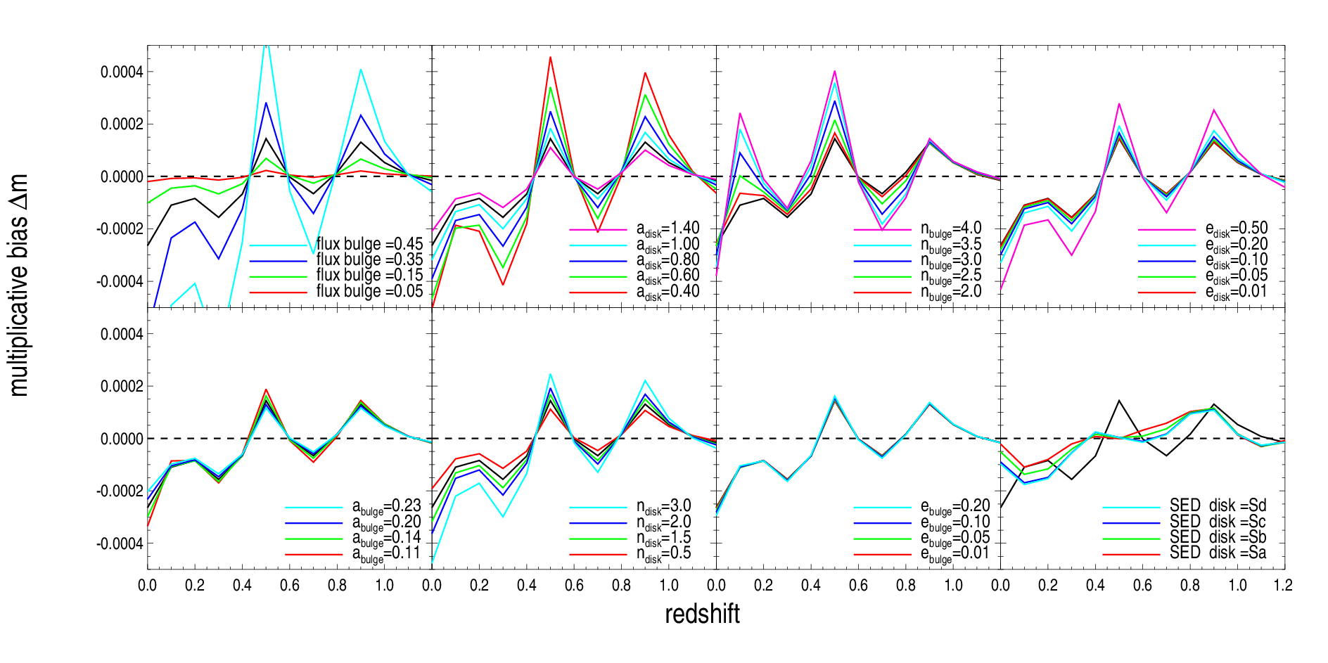
Many parameters contribute to the actual spatial colour variations and it is therefore useful to examine how the bias changes as a function of the bulge and disk characteristics. To do so, we take galaxy B and vary one parameter at a time, keeping all others constant (using PSF1 and adopting ). The results are presented in Figure 5. We find that the bias depends most strongly on the flux of the bulge, but also depends on the size of both bulge and disk. It does not depend much on their ellipticity .
In general the bias values range between values of a few times to a few times . Note that in all panels the rest-frame colour of the galaxies is the same, except when we vary the fraction of the flux in the bulge (top left panel) or when we change the SED (bottom right panel). These results confirm what we concluded based on Equations (9, 10), i.e. the bias is foremost a function of the colour of the galaxy. Whereas the absolute value of the bias increases when the size of the source galaxy decreases, the changes as a function of the parameters are similar for all galaxies in Table 3. The reference galaxy and its smaller version both have a relatively large disk, which leads to a large FWHM at (see Table 3). Therefore we also consider two galaxies with a smaller FWHM: B4 and S4. The ratio at is 1.3 and 1.1 for B4 and S4, respectively. As one can see from Figure 6, the bias is a very strong function of this ratio: it is smaller than for a well-resolved galaxy and can become a few percent for a galaxy which is about the size of the PSF.
Figure 6 also shows that for all galaxies in Table 3 the bias is larger for the reference Gaussian PSF (black points) than for the more realistic PSF3 (blue diamonds). However, the behaviour of the bias as a function of is very similar for the two PSF models. In particular, the bias is still a few percent when . Note, however, that in the case of a PSF as small as that of Euclid we do not expect galaxies with observed sizes similar to the PSF (Massey et al., 2012, e.g.). For this reason, a characteristic size of about 1.4 can be considered representative for the Euclid galaxy sample. For such galaxies we expect a bias of a few times .
 |
5 Calibration of the bias
In order to obtain accurate constraints on cosmological parameters, the multiplicative bias for the Euclid cosmic shear analysis needs to be less than (Massey et al., 2012; Cropper et al., 2012). The results presented in the previous section suggest, however, that the spatial variation of the SED will lead to multiplicative biases in the ellipticity that exceed the allowed range in the case of Euclid. Hence a way to mitigate the problem of colour gradients is required.
In principle it should be possible to model the colour gradients (and thus determine the bias) using resolved images of galaxies taken in different filters. This approach was already suggested by Voigt et al. (2012). Unfortunately, many factors influence the quality of the results. The accuracy with which one can model the bias depends on the properties of these images: signal-to-noise ratio, resolution, pass-band characteristics, number of filters, properties and knowledge of the PSF.
Voigt et al. (2012) explored the possibility of a calibration sample, covering the full range of properties of the source galaxies, for which the bias can be determined. Following their work, we examine this route in more detail, starting with the question what data are required to determine the bias observationally.
5.1 Approximated SED reconstruction
To quantify the colour gradient bias, resolved observations in at least two filters are needed. In this section we explore how well one can reconstruct the spatial colour distribution of a galaxy when observations in only two bands of that galaxy are available. For each of the narrower filters, we define the observed image:
| (22) |
We use the observed image in each filter, , to derive the approximated intensity that we need to estimate the bias. We will for the moment ignore the fact that a galaxy observed in the narrower filters has already been convolved by a PSF (i.e. we take it to be a -function). This will be addressed in the next section. In addition we make the assumption that for each pixel the SED can be interpolated linearly:
| (23) |
The coefficients can be determined for each pixel by solving a linear system of equations:
| (24) |
Once we obtain the approximated intensity we use it to estimate the bias induced by the colour gradients in the same way we have done previously.
As shown below, HST observations represent the best available sample to study the impact of colour gradients on the shear estimation, which explains our choice of filters. We use the spatial resolution and transmission for the F606W and F814W filters (see left panel of Figure 2). Note that this procedure can be applied to other sets of resolved observations taken in two or more filters, although the accuracy of the results will vary. The use of more bands allows one to estimate the SED more accurately, for example by using higher order polynomial interpolations.
In the presence of noise, as is the case for real data, it will be more challenging to reconstruct the spatial colour distribution by interpolation. In the case of Euclid we do not expect this to be a major issue as the galaxies used as calibration sample will have a relatively high signal-to-noise ratio in typical HST observations. Alternatively, one might consider ways to reduce the impact of the noise, for example by using a shapelet decomposition (Refregier, 2003; Kuijken, 2006).
Having fixed the properties of the two filters, we can compute the difference between the bias for the Euclid broad-band observations and the bias reconstructed using the linear interpolation from F606W and F814W observations. Figure 7 shows the results for model galaxy B as a function of redshift when we vary the parameters as was done for Figure 5. We find that we are able to recover the bias with an accuracy of a few times .
We note that generally shows the same features and that its amplitude is proportional to the input bias. This stems directly from the fact that the linear interpolation cannot reproduce the Irr SED accurately enough (see Figure 1). The main reason for this is associated with the presence of emission lines in the range , although this is not the only reason. Not surprisingly, the linear interpolation cannot reproduce any of the SEDs perfectly over the large range in wavelength covered by the Euclid pass-band. The linear interpolation fails to capture some of the features of the SEDs visible at and the Balmer break at .
Hence the inaccuracy in modelling the SED at each position leads to a residual bias which is a strong function of redshift. However, we note that Figure 7 exacerbates the problem because the local Irr SED is always the same and the linear interpolation fails coherently. In practice, the linear interpolation will sometimes overestimate and sometimes understimate the bias such that the average bias as a function of redshift might still be estimated correctly and the residuals uncorrelated. The SED also depends on the age of the stellar population, the metallicity, the dust extinction, and the velocity dispersion; all aspects we have neglected. For instance, the bottom-right panel of Figure 7 shows that changing the Irr SED used for the disk to any of the Sa-Sd spectra changes the residual bias substantially.
Finally, it is possible to improve on these results by performing an SED fit instead of a linear interpolation. This might be feasible especially in the case of low redshift galaxies for which multi-colour observations are available and can be used to put tight constrains on the local SED. This could significantly improve the accuracy on the estimated bias at low redshift and help to reduce the residual bias at higher redshifts.
5.2 Effect of the native PSF
Since the images we use to evaluate the colour gradient-induced bias have been convolved with a PSF themselves, the procedure used to retrieve the local SED is more complicated in practice. Accounting for the PSF, Equation (22) changes to
| (25) |
In Fourier space we obtain a linear system of equations which we can solve to obtain and , the Fourier transformed maps of the linear coefficients to approximate the local SED. Solving a linear system in Fourier space corresponds to performing a deconvolution. This will therefore cause loss of information, as we cannot reconstruct scales that are smaller than the PSF. Note that this system of equations can be expanded to more filters, and higher order interpolations. The filters might also have different PSFs.
6 Euclid bias modelling with HST filters
In the previous section we have shown that it is possible to quantify the effect of colour gradients using resolved observations in at least two filters. A complication is that one needs to deconvolve the galaxies to account for the native PSF of the narrower filters. This will reduce the overall accuracy of the measurement of the colour gradient bias for two reasons. First of all, solving the system of equations (25) for the local SED is equivalent to a deconvolution, implying that there is an upper limit to the spatial frequencies we can recover. Secondly, the native PSF we need to correct for is not perfectly known.
Since deconvolution algorithms have intrinsic limitations which depend on the size of the PSF, a small PSF is always preferable. Amongst currently available data, HST observations are therefore the most suitable to model colour gradients. As can be seen in Figure 8, the characteristic size of the Euclid PSF is twice the HST PSF. This stems directly from the fact that the diameter of the Euclid mirror is about half of the size of the HST mirror, . Despite its small size, there is a loss in accuracy caused by the HST PSF. Furthermore, the HST PSF does vary as a function of position and time, which can be modelled with finite accuracy. The impact of both complications are quantified below.
We generate images of the HST PSF at different positions and for various focus configurations using the Tiny-Tim software (Krist et al., 2011). The PSF images have a pixel size of and are sampled as a function of wavelength with a step . When convolving the images of the source with the HST PSF, we approximate the PSF to the closest one in instead of interpolating between the various PSF images.
The top panel of Figure 8 shows our nominal HST PSF profile, which is the one in the middle of the first ACS chip, without defocus, for . We compare this profile to those obtained by changing the position across the camera and the focus. In the bottom panel we show the same HST PSF profiles but for . Note that we ignore the camera distortion, as it does not alter colour gradients and can be corrected for before modelling the bias.
Both focus and position changes from the nominal configuration increase the half-light radius of the PSF, but in different ways. The change of the focus (upper panel of Figure 8) does not affect the core of the PSF but it affects the wings, which become larger (effectively the PSF profile is slightly suppressed at small scales and boosted at larger scales). Changing the position affects both the core and the wings of the PSF. This is the result of a change in the diffusion coefficients which increases the overall characteristic size of the PSF. In both cases the effect is very small and we do not expect the final results to depend significantly on the position nor on the focus.
 |
6.1 PSF deconvolution
We use the PSFs generated with Tiny-Tim for the nominal focus and position to create images for model galaxies B and S. We estimate the bias without accounting for the PSF and present the results in Figure 9 (red lines). Comparison with the true bias (black lines) shows that ignoring the PSF leads to an underestimate of the bias because the native PSF blurs the colour gradients. As expected, the effect is larger when the galaxy is smaller (right panel).
If we instead use Equation (25) to reconstruct the approximated intensity profiles we obtain the blue solid lines in Figure 9. Hence, when the convolution by the HST PSF is accounted for, we recover the original bias quite well, as shown in the bottom panels where we plot the difference between the original bias and the estimated one. For the galaxy B we are able to recover the bias within an accuracy of ; as expected, the performance is worse for the S galaxy. This difference includes the error made by approximating the local SED with a linear function and it is interesting to note that the residuals for both galaxies are similar to the one estimated in Section 5, where we ignored the PSF of the narrower band data. This suggests that the linear interpolation of the SED is still the main limitation and that HST data are suitable to model the bias induced by the presence of colour gradients. As a caveat we note that the deconvolution step will be more complicated in practice due to the presence of noise in real data.
 |
6.2 Imperfect PSF knowledge
The HST PSF cannot be modelled perfectly because it varies with time. The resulting error in the PSF model will lead to an error in the estimate of the colour gradient bias. We estimate the impact of this by examining the variation in the bias for a range of HST PSFs. Under the assumption that the deconvolution and the SED interpolation work perfectly, the loss of accuracy is given by the dispersion between the bias estimates for the various PSFs. This allows us to estimate an upper limit to the accuracy due to the errors in the HST PSF model.
 |
To do so, we evaluate the bias for slightly different PSFs but without deconvolving the PSF. We generate PSFs using Tiny Tim for various focus configurations and camera positions and measure the resulting colour gradient bias using Equation (24). The top panels of Figure 10 show the amplitude of the bias for a few positions and defocus values. For reference we also show the true bias (black solid line). The difference between the bias for the reference HST PSF and the bias obtained when the defocus and the position are changed is presented in the bottom panels. Note that the differences are always smaller that and always positive. This is because the changes in position and focus both increase the PSF size (and thus the absolute value of the bias). As expected, the impact of variations of the HST PSF are larger for galaxy S. For galaxy B, the changes in the bias values are about , whereas for the galaxy S they are about in the worst case.
Were it possible to perform a perfect deconvolution, ignoring PSF variations as a function of position and focus would lead to an extra error term. This error can be roughly estimated as the product of the dispersion from the various focus and position configurations, multiplied by the ratio between the true and recovered bias (black and orange lines, respectively). In practice the PSF as a function of position and focus can be determined reasonably well (see for example Rhodes et al. 2007; Schrabback et al. 2010) and the error is expected to be significantly smaller than what is shown in Figure 10. Hence, the limited accuracy of the model for the HST PSF is not an important source of error.
7 Calibration of the bias
Voigt et al. (2012) proposed to use HST observations of galaxies to determine the mean bias as a function of galaxy properties. The precision with which this can be done depends on the intrinsic variation in galaxy properties, which in turn drives the size of the sample of galaxies that is needed. In this section we examine whether the HST archive contains a sufficient number of resolved galaxies observed in at least two bands to model the bias with the precision required for Euclid’s science objectives.
Throughout this paper we have made realistic but rather conservative assumptions in order to estimate the bias using simulated bulge plus disk galaxies that by design showed significant colour gradients. The actual amplitude of the bias, however, needs to be derived using actual observations. A preliminary analysis based on 12,000 galaxies in the Extended Groth Strip (EGS, Davis et al. 2007) suggests an average value of in the worst cases, with an uncertainty of a few times computed in redshift bins each containing about 500 galaxies (Huang et al. in prep.).
The average bias is larger than the measured by Voigt et al. (2012) using their full dataset comprising galaxies. A source for this difference is our use in this paper, and in the preliminary analysis of EGS data, of a PSF that has a larger size and a stronger dependence than the one used by Voigt et al. (2012) which is closer to Euclid’s one. Additional differences might arise from the fact that we use different shear estimates. Furthermore, as pointed out by Voigt et al. (2012), their selection of galaxies may not be very representative. For instance, the EGS dataset may contain a fraction of galaxies with red bulges larger than the ones in the Simard et al. (2002) catalogue; as shown in Figure 6 of Voigt et al. (2012), selecting galaxies with a redder bulge enhances the bias to . Voigt et al. (2012) estimate a dispersion in the bias of for the whole sample, which suggests that about a thousand33 3 Voigt et al. (2012) quote a number of galaxies that is ten times larger to account for possible limitations in the accuracy of their analysis, which is based on a small sample of galaxies with a bulge and disk decomposition. galaxies per redshift bin are needed to obtain . The error on the average we obtain from the preliminary EGS analysis agrees with these values. As shown in Table 4, the HST archive contains enough galaxies to reach this precision.
7.1 Residual bias correlations
The bias depends on the intrinsic properties of the galaxies, which in turn depend on environment. The colour gradient bias will therefore vary spatially. A simple correction using the average bias for each tomographic bin may therefore not be sufficient, and still lead to a spurious signal in the two-point cosmic shear statistics.
We assess the residual bias on the correlation function as follows. We compute the two-point ellipticity correlation function selecting sources belonging to the same redshift bin:
| (26) |
where the ensemble average is meant as an average over all pairs with distance and and indicate the tangential and the -degree rotated components of the estimated shear projected along the line connecting the pair of galaxies (Bartelmann & Schneider, 2001, see for example). We define , the relative bias in the correlation function:
| (27) |
Based on the breakdown presented in Cropper et al. (2012) we assume that Euclid’s science objectives can be achieved if the value is smaller than for all angular scales . This limit allows us to estimate the required minimum size of the calibration sample that is used to determine the average colour gradient bias as a function of galaxy properties and redshift.
Since we lack observational results we use simulations to conservatively estimate the impact of the spatial variation in the colour gradient bias. In the following we use model galaxy S, which has a bias of a few times and an observed FWHM of about , typical of a galaxy in the Euclid survey.
To simulate the properties of galaxies in the Euclid survey and the calibration sample we use ray tracing simulations produced using the Millennium Simulation (Hilbert et al., 2009; Springel et al., 2005). The ray tracing simulations comprise lines of sight, each covering . For each galaxy we know the shear, the redshift and magnitudes in various SDSS bands. To simulate the depth of the Euclid catalogue we add the , and a third of the fluxes of the SDSS bands and select galaxies brighter than . The resulting density is , in agreement with expectations. We use the SDSS values to define the colour of each galaxy.
 |
7.2 Size of the calibration sample
We searched the HST archive for ACS observations in at least two (suitable) filters. The results are listed in Table 4, where we note that we also include scheduled observations. The sample contains approximately of F606W and F814W data including EGS (Davis et al., 2007) and the overlap of CANDLES (Grogin et al., 2011) with either COSMOS (Scoville et al., 2007) and GOODS (Giavalisco et al., 2004). We have also included the area of GEMS (Rix et al., 2004) data that does not overlap with either GOODS or CANDLES. For this part of the GEMS data we have F850LP observations which are shallower and slightly redder than the F814W data; these can be also used to calibrate colour gradients, but the lower signal-to-noise is expected to reduce the accuracy. This results in a total area of containing about galaxies for which we can determine the colour gradient bias observationally.
The data listed in Table 4 were obtained as part of several surveys. Including single ACS pointings as well would increase the area by another . Finally, dedicated deep Euclid observations of the area covered by STAGES (Gray et al., 2009) and COSMOS would increase the sample by more than a factor of three. The full benefit of the latter observations requires more study because the Euclid PSF size is larger and pass-band broader. In the following we therefore conservatively assume that we can measure the colour gradient bias using HST observations of galaxies.
| Name | Area () | Number of galaxies |
|---|---|---|
| EGS | 650 | 18000 |
| CANDELS/UDS | 198 | 6000 |
| CANDELS/COSMOS | 6000 | |
| CANDELS/GOODS-CDFS | 9000 | |
| CANDELS/GOODS-NORTH | 5500 | |
| GEMS/CANDLES+GOODS | (F850LP) | 15500 |
| total | 62000 |
7.3 Bias model
To each galaxy in the simulation we assign a bias , which is a function of colour and redshift. Including the colour dependence is important to capture the fact that galaxy colour depends on environment. The value for the bias is obtained by taking the S galaxy and varying the fraction of light in the bulge as we did in the top-left panel of Figure 5. Note that increasing the fraction of light in the bulge without changing its size results in redder galaxies with an unrealistically small but very bright bulge. To avoid this, we increase the size of the bulge accordingly, thus accounting for the increase in its flux. The galaxy S has a bulge size of which contains 25% of the light; we set of the bulge to that of the disk () when the flux of the bulge is (note that in this case we have an elliptical galaxy with no colour gradients) and create all other cases using a linear relation between flux and size.
Once we have created this set of model galaxies, we derive their colours by integrating the flux over the SDSS and filters. The resulting colours are generally too blue compared to the galaxies in the Millennium Simulation. These differences are likely caused by differences in the adopted SEDs. The change in colour with redshift for our model early-type galaxies is the same as that of the red Millennium galaxies. Thus, we correct for this offset in colour by shifting them slightly to match the results from the Millennium Simulation.
 |
The left panel of Figure 11 shows the colour distribution of the simulated Euclid-like galaxies for three redshift bins. For each redshift bin we also show the bias as a function of the observed colour. The blue (red) lines indicate the bias for a galaxy at the lower (upper) limit of the respective redshift bin. In all cases the bias reaches a maximum value when the bulge contains about 20-30% of the light.
The bias assigned to each galaxy in the Millennium Simulation is computed by interpolating the value of the multiplicative bias as a function of the colour at the redshift of the galaxy. The average bias as a function of redshift is presented in the right panel of Figure 11. Figure 11 shows that , similar to what is found from the preliminary EGS analysis. The dispersion of the simulated bias, however, is about , smaller than that found from the EGS analysis. To ensure that our estimates remain conservative, we increase the variance of accordingly: we include an additional spread in the bias sampled by a Gaussian of width .
This results in a simulated data set where the bias depends on redshift and colour with an extra variance to account for variations as a function of other parameters (such as ellipticity and size). These estimates were used to compute the errors on the mean bias as a function of redshift presented in Figure 11, where we assume a calibration sample of galaxies ( of which have ).
7.4 Effect on the ellipticity correlation function
So far we have limited the discussion to the impact of colour gradients on the multiplicative bias . As the bias is related to the correction for the PSF, we expect the additive bias to be affected as well. In this more general case, the shear estimate for the -component is given by:
Inserting this expression into Equation (26) we find that the measured correlation function can be expressed as:
| (28) |
where and quantify the correlations of and , respectively, as a function of angular separation. The relative bias in the correlation function is thus given by:
| (29) |
Massey et al. (2012) derived expressions for the various sources of multiplicative and additive bias and showed that the contributions to and caused by colour gradients are related through:
| (30) |
where is the -component for the PSF ellipticity. Following Massey et al. (2012), we assume . Hence we have , where is the ellipticity correlation function of the PSF anisotropy. Because our definition of ellipticity by Equation (15) differs from the one used by Massey et al. (2012), we have whereas we adopt for the PSF ellipticity44 4 This corresponds to the maximum value for the polarisation of allowed for the Euclid PSF (Laureijs et al., 2011; Cropper et al., 2012)., which is an extremely pessimistic scenario.
Although is smaller than , Equation (29) shows that the additive bias can become dominant on large scales if the PSF ellipticity correlation function does not vanish sufficiently quickly. In our case the PSF orientation is constant across the field, which implies that for any given value of there will be a scale for which , unless vanishes faster than . This scale is smaller for low-redshift sources for which the cosmic shear signal is smaller.
This large-scale signal provides a way to estimate the amplitude of the colour-gradient induced bias directly from the Euclid dataset by measuring the correlation between the ellipticity of stars and the PSF-corrected ellipticity of galaxies (i.e. the shear). This correlation is commonly used as a diagnostic to ensure that the PSF anisotropy is well corrected (Heymans et al., 2012, e.g.). For this reason one would rather not use this residual signal to correct for colour gradients. However, in the case of colour gradients we do not need to correlate galaxies and stars in the same field: the colour gradient bias will be proportional to the PSF anisotropy, so that residuals of independent fields will be correlated. Note that in the absence of colour gradients these correlations are supposed to vanish if the correction for PSF anisotropy is accurate on average.
| redshift only | redshift and colour | |||||
|---|---|---|---|---|---|---|
 |
The calibration sample is used to obtain an estimate for , the average value of the bias for a particular selection of sources, which is used to correct the shear signal for these galaxies. Hence the relevant quantity becomes , the residual bias for each galaxy after correction. After removing the average bias, we can rewrite Equation (29) to obtain:
| (31) |
where is the correlation function of the residuals . As for the uncorrected case, the first term is related to the multiplicative bias, while the second term corresponds to the additive bias.
7.5 Bias estimation
We assume the calibration sample to be a contiguous patch with the same area as the total area of the datsets presented in Table 4. This increases the sampling variance compared to what one would obtain from several independent fields. Hence, our estimates are conservative. The model for the bias from this calibration subsample is then used to correct the bias for the whole survey. To estimate the sampling variance we generate 32 independent realisations where each time a different location for the calibration sample is selected.
We create simulated shear catalogues for three different scenarios. In the first scenario we do not correct for the bias, whereas in the second case we use the calibration sample to derive an average bias value as a function of the redshift. We sample the bias in steps of . In the third case we use the calibration sample to determine the average bias as a function of redshift and observed colour. We sample the bias in steps of and 15 bins of colour of width 0.10 covering the range between .
We start by exploring the and contributions to the bias in the correlation function separately. The left panel of Figure 12 shows the amplitude of for the tomographic bin , which can be compared to the cosmic shear signal (black line). Since the PSF orientation is constant, is always positive, its asymptotic value is and there is a scale for which the value of becomes larger than the cosmological signal. This happens at scales larger than even for the smallest redshift bin. In reality is expected to be a factor smaller as the Euclid PSF anisotropy in the currently agreed optical design (c. 2011-2012) is supposed to be about only in the corners while it is about in most of the field of view. Additionally, the PSF pattern varies across the field, so that decreases quickly and it is expected to be very small on scales that are larger than the field of view (indicated in the left panel of Figure 12 and in Figure 13 by the magenta dashed lines).
As indicated by the green triangles in Figure 12, the value for is reduced by two orders of magnitude at large angular scales when we use the average bias as a function of redshift to correct the colour gradient bias. The improvement is smaller on small scales, where the clustering of galaxies is important. This is remedied by modelling the bias as a function of colour and redshift (blue triangles). The error bars shown in Figure 12 have been computed from the 32 realisations and include sampling variance.
The right panel of Figure 12 shows the value of when . As expected, when no correction is applied, the overall bias is about . Since , the signal is suppressed (i.e ). Once again, correcting the average bias as a function of redshift improves the results. Including the colour dependence improves the results even further to a level below the requirement of (indicated by the dotted line).
Figure 13 shows , for three redshift bins. If the colour gradient bias is ignored, has a minimum due to the competition between the multiplicative and additive terms, which have an opposite effect on the observed ellipticity correlation function. The location of the minimum indicates the scale where the additive bias starts to dominate. Similarly to what we found in Figure 12, correcting the measured shear by the average bias as a function of redshift reduces the amplitude of the residual bias on the correlation function. Taking into account the dependence upon the observed colour reduces this residual further, in particular for small angular scales. For reference we indicate with a dotted line the maximum value for allocated to achieve Euclid’s science objectives.
The measurements at different angular scales in Figure 13 are correlated, which complicates a simple interpretation of the significance of the results. We therefore computed the average residual bias, accounting for the correlation between the angular scales using the covariance matrix computed from the simulations. The results are reported in Table 5 for the three redshift bins after correcting the bias either as a function of redshift or as a function of both redshift and colour. We derive the average residual bias for three different ranges: the full range of scales, i.e. ; eliminating scales which will not be included in the cosmological analysis, i.e. ; eliminating scales larger than the Euclid field-of-view, i.e. . In all cases we find that modelling the bias as a function of colour and redshift produces better results than modelling the bias as a function of redshift only. With this correction we obtain residual biases that are consistent (within ) with the maximum allowed value (i.e. ). A more realistic model for the PSF anisotropy would result in a significantly smaller residual bias, especially on large scales.
Overall these results demonstrate that the HST archive contains a sufficient number of galaxies observed in at least two suitable bands to calibrate the colour gradient-induced bias to the precision required for Euclid. To simulate the spatial variation of the bias using the Millennium Simulation, we assumed that the colour is the main parameter to consider. We thus ignored the fact that the bias also depends on other parameters such as its ellipticity, Sersíc index, etc., as is evident from Figure 5. This has the effect of reducing the simulated scatter in the bias for a given colour and redshift, but we accounted for this by including an intrinsic scatter in order to match results from a preliminary analysis of EGS data (Huang et al., in prep.). We note that we assumed a rather pessimistic PSF anisotropy and PSF size and therefore are confident that our estimates are in fact conservative. On real data, we can can test further bias dependencies and model it as a function of an optimal set of parameters. The efficiency of the correction can be tested and eventually improved by dividing the Euclid dataset in subsamples and comparing the differences in shear distributions measured on these subsamples.
8 Conclusions
Euclid will measure the cosmic shear signal with unprecedented precision (Laureijs et al., 2011). To do so it will measure galaxy shapes from images observed in a rather broad filter. In combination with the wavelength dependence of the PSF this leads to biases in the shape measurements because the colours of galaxies vary spatially. To ensure that the constraints on cosmological parameters are not compromised it is important to quantify this ‘colour gradient’ bias and examine possible approaches to mitigate the problem.
In this paper we show how the spatial variation of the colour of a galaxy generally leads to a bias in the measurement of its shape. In the case of unweighted moments the PSF can be removed without introducing any bias. In practice, in order to suppress the noise, shear measurement methods use a weight function that assigns more weight to the inner regions. Consequently, the bias depends on the choice of the weight function and is therefore generally method-dependent. We derive results for moment-based methods, but note that our findings are also applicable to methods that fit galaxy models to the data.
We showed analytically that the amplitude of the bias scales proportional to the square of the width of the filter used for the measurement. We studied in detail how the bias depends on the characteristics of the galaxies and the PSF using model galaxies. The amplitude of the bias depends strongly on the ratio of the observed FWHM of the galaxy to the FWHM of the PSF, with a larger PSF leading to a larger bias. The bias can be as large as a few percent if the observed galaxy is about the size of the PSF, while it decreases rapidly to only a few times when the galaxy size is 1.6 times the PSF size. Given the small size of the Euclid PSF and the magnitude limit of , the observed galaxies will generally have an observed FWHM which is larger than the PSF. The bias depends on the bulge and disk sizes, on the ellipticity, but it depends most strongly on the colour of the galaxy.
It is possible to determine the bias observationally using spatially resolved data observed in at least two filters. We focus on the particular case of HST observations in F606W and F814W, which are best suited for this purpose. We quantify the limitations in modelling the local SED using only two filters taking into account the HST PSF. We find that the linear interpolation we use to approximate the local SED is the main source of error. This could be improved in principle by performing a local SED fit. This might be possible especially for low redshift galaxies where we have resolved observations in various colours. Errors in the model for the HST PSF have a very minor impact. Our results therefore indicate that we can model the bias due to colour gradients using HST observations with an accuracy of a few times for a typical galaxy used in the Euclid weak lensing analysis.
To determine the average bias with sufficient precision requires a representative sample of galaxies. Voigt et al. (2012) suggested that a sample of about thousand galaxies per redshift bin would be sufficient to determine the bias with a precision of . This has been confirmed by a preliminary analysis using EGS data (Huang et al. in prep.). The amount of archival HST data observed in at least two bands is sufficient for this.
A complication arises from the fact that the bias depends strongly on the colour. As a result the clustering of galaxies will lead to spatial variations in the bias. In this case an average correction for each redshift bin may still lead to biases in the two-point ellipticity correlation function. To examine the impact of this second order effect we used a ray-tracing catalogue based on the Millennium Simulation. We find that correcting the bias as a function of both redshift and colour using a contiguous patch containing about 40,000 galaxies is sufficient to correct the bias to the accuracy required for the Euclid two-point shear tomography. This is a conservative estimate of the number of galaxies in the HST archive at the time of Euclid’s launch. We therefore conclude that the presence of colour gradients in galaxies is not a limiting factor for the Euclid cosmic shear analysis.
Acknowledgements
We would like to thank Gary Bernstein, Christopher Hirata, Jérôme Amiaux and Frederic Courbin and in general, the members of the Euclid Consortium for helpful discussions. ES and HH acknowledge the support of the Netherlands Organization for Scientific Research (NWO) through a VIDI grant and the support from the European Research Council under FP7 grant number 279396. BJ acknowledges support by a UK Space Agency Euclid grant and by STFC Consolidated Grant ST/J001422/1. TK was supported by a Royal Society University Research Fellowship. JR was supported by JPL, run by Caltech under a contract for NASA. TS acknowledges support from NSF through grant AST-0444059-001, SAO through grant GO0-11147A, and DLR through grant FKZ 50 QE 1103. MV acknowledges support from the Netherlands Organization for Scientific Research (NWO) and from the Beecroft Institute for Particle Astrophysics and Cosmology. This material is based upon work supported in part by the National Science Foundation under Grant No. 1066293 and the hospitality of the Aspen Center for Physics.
References
- Bartelmann & Schneider (2001) Bartelmann M., Schneider P., 2001, Phys. Rep., 340, 291
- Bridle et al. (2010) Bridle S. et al., 2010, MNRAS, 405, 2044
- Bridle et al. (2009) Bridle S. et al., 2009, Annals of Applied Statistics, 3, 6
- Bridle et al. (2002) Bridle S. L., Kneib J.-P., Bardeau S., Gull S. F., 2002, in The Shapes of Galaxies and their Dark Halos, Natarajan P., ed., pp. 38–46
- Capaccioli (1989) Capaccioli M., 1989, The world of galaxies, H.G. Corwin L. B., ed. Springer-Verlag, Berlin
- Coleman et al. (1980) Coleman G. D., Wu C.-C., Weedman D. W., 1980, ApJS, 43, 393
- Cropper et al. (2012) Cropper M. et al., 2012, MNRAS, submitted, arXiv:1210.7691
- Cypriano et al. (2010) Cypriano E. S., Amara A., Voigt L. M., Bridle S. L., Abdalla F. B., Réfrégier A., Seiffert M., Rhodes J., 2010, MNRAS, 405, 494
- Davis et al. (2007) Davis M. et al., 2007, ApJ, 660, L1
- Giavalisco et al. (2004) Giavalisco M. et al., 2004, ApJ, 600, L93
- Gray et al. (2009) Gray M. E. et al., 2009, MNRAS, 393, 1275
- Grogin et al. (2011) Grogin N. A. et al., 2011, ApJS, 197, 35
- Heymans et al. (2006) Heymans C. et al., 2006, MNRAS, 368, 1323
- Heymans et al. (2012) Heymans C. et al., 2012, MNRAS, 427, 146
- Hilbert et al. (2009) Hilbert S., Hartlap J., White S. D. M., Schneider P., 2009, A&A, 499, 31
- Hoekstra et al. (2000) Hoekstra H., Franx M., Kuijken K., 2000, ApJ, 532, 88
- Hoekstra & Jain (2008) Hoekstra H., Jain B., 2008, Annual Review of Nuclear and Particle Science, 58, 99
- Hu (1999) Hu W., 1999, ApJ, 522, L21
- Hu (2002) Hu W., 2002, Phys. Rev. D, 66, 083515
- Kacprzak et al. (2012) Kacprzak T., Zuntz J., Rowe B., Bridle S., Refregier A., Amara A., Voigt L., Hirsch M., 2012, ArXiv:1203.5049
- Kaiser et al. (1995) Kaiser N., Squires G., Broadhurst T., 1995, ApJ, 449, 460
- Kitching et al. (2010) Kitching T. et al., 2010, ArXiv:1009.0779
- Kitching et al. (2012a) Kitching T. D. et al., 2012a, MNRAS, 423, 3163
- Kitching et al. (2008) Kitching T. D., Miller L., Heymans C. E., van Waerbeke L., Heavens A. F., 2008, MNRAS, 390, 149
- Kitching et al. (2012b) Kitching T. D. et al., 2012b, ArXiv:1204.4096
- Krist et al. (2011) Krist J. E., Hook R. N., Stoehr F., 2011, in Society of Photo-Optical Instrumentation Engineers (SPIE) Conference Series, Vol. 8127, Society of Photo-Optical Instrumentation Engineers (SPIE) Conference Series
- Kuijken (2006) Kuijken K., 2006, A&A, 456, 827
- Laureijs et al. (2011) Laureijs R. et al., 2011, ArXiv:1110.3193
- Massey et al. (2007) Massey R. et al., 2007, MNRAS, 376, 13
- Massey et al. (2012) Massey R. et al., 2012, MNRAS, accepted, arXiv:1210.7690
- Melchior & Viola (2012) Melchior P., Viola M., 2012, MNRAS, 424, 2757
- Melchior et al. (2011) Melchior P., Viola M., Schäfer B. M., Bartelmann M., 2011, MNRAS, 412, 1552
- Miller et al. (2012) Miller L. et al., 2012, MNRAS, submitted, ArXiv:1210.8201
- Miller et al. (2007) Miller L., Kitching T. D., Heymans C., Heavens A. F., van Waerbeke L., 2007, MNRAS, 382, 315
- Munshi et al. (2008) Munshi D., Valageas P., van Waerbeke L., Heavens A., 2008, Phys. Rep., 462, 67
- Nakajima & Bernstein (2007) Nakajima R., Bernstein G., 2007, AJ, 133, 1763
- Paulin-Henriksson et al. (2009) Paulin-Henriksson S., Refregier A., Amara A., 2009, A&A, 500, 647
- Refregier (2003) Refregier A., 2003, MNRAS, 338, 35
- Refregier et al. (2012) Refregier A., Kacprzak T., Amara A., Bridle S., Rowe B., 2012, MNRAS, 425, 1951
- Rhodes et al. (2007) Rhodes J. D. et al., 2007, ApJS, 172, 203
- Rix et al. (2004) Rix H.-W. et al., 2004, ApJS, 152, 163
- Schrabback et al. (2010) Schrabback T. et al., 2010, A&A, 516, A63
- Scoville et al. (2007) Scoville N. et al., 2007, ApJS, 172, 38
- Simard et al. (2002) Simard L. et al., 2002, ApJS, 142, 1
- Springel et al. (2005) Springel V. et al., 2005, Nature, 435, 629
- Valdes et al. (1983) Valdes F., Jarvis J. F., Tyson J. A., 1983, ApJ, 271, 431
- Voigt et al. (2012) Voigt L. M., Bridle S. L., Amara A., Cropper M., Kitching T. D., Massey R., Rhodes J., Schrabback T., 2012, MNRAS, 421, 1385