The Higgs Boson in the Standard Model
—
From LEP to LHC: Expectations, Searches, and Discovery of a Candidate

The Lagrangian ${\cal{L}}_{\mathrm{SM}}$ of the SM can be divided into four different parts,

$${\cal{L}}_{\mathrm{SM}}={\cal{L}}_{\mathrm{YM}}+{\cal{L}}_{\mathrm{ferm}}+{\cal{L}}_{\mathrm{H}}+{\cal{L}}_{\mathrm{Yuk}},$$

(1)

which will be discussed one by one in the following. We start with the first two, which contain the dynamics of the gauge bosons and matter fermions as predicted by the unbroken gauge symmetry, before we turn to the latter two which involve the Higgs field.

The Yang–Mills part ${\cal{L}}_{\mathrm{YM}}$ describes the genuine dynamics of the gauge fields, i.e. their free propagation as well as their self-interactions,

$${\cal{L}}_{\mathrm{YM}}=-\frac{1}{4}W^{i}_{\mu\nu}W^{i,\mu\nu}-\frac{1}{4}B_{\mu\nu}B^{\mu\nu}-\frac{1}{4}G^{a}_{\mu\nu}G^{a,\mu\nu},$$

(2)

where

	$\displaystyle W^{i}_{\mu\nu}$	$\displaystyle=$	$\displaystyle\partial_{\mu}W^{i}_{\nu}-\partial_{\nu}W^{i}_{\mu}-g\epsilon^{ijk}W^{j}_{\mu}W^{k}_{\nu},\qquad i,j,k=1,2,3,$
	$\displaystyle B_{\mu\nu}$	$\displaystyle=$	$\displaystyle\partial_{\mu}B_{\nu}-\partial_{\nu}B_{\mu},$
	$\displaystyle G^{a}_{\mu\nu}$	$\displaystyle=$	$\displaystyle\partial_{\mu}G^{a}_{\nu}-\partial_{\nu}G^{a}_{\mu}-g_{\mathrm{s}}f^{abc}G^{b}_{\mu}G^{c}_{\nu},\qquad a,b,c=1,\dots,8,$		(3)

are the field-strength tensors of the gauge fields $W^{i}_{\mu}$ for the SU(2)_I group of the weak isospin $I_{\mathrm{w}}^{i}$, $B_{\mu}$ for the U(1)_Y of weak hypercharge $Y_{\mathrm{w}}$, and $G^{a}_{\mu}$ for the SU(3)_c of colour. The respective gauge couplings of these groups are denoted $g$, $g^{\prime}$, and $g_{\mathrm{s}}$, and the structure constants of the non-abelian groups SU(2) and SU(3) are $\epsilon^{ijk}$ and $f^{abc}$, following the usual notation.

The interaction of the gauge fields with the fermions is encoded in

$${\cal{L}}_{\mathrm{ferm}}={\mathrm{i}}\overline{\Psi}_{L}\mathchoice{\hbox to0.0pt{\hss$\displaystyle/$\hss\kern-8.55695pt}\hbox{$\displaystyle D$}}{\hbox to0.0pt{\hss$\textstyle/$\hss\kern-8.55695pt}\hbox{$\textstyle D$}}{\hbox to0.0pt{\hss$\scriptstyle/$\hss\kern-6.75377pt}\hbox{$\scriptstyle D$}}{\hbox to0.0pt{\hss$\scriptscriptstyle/$\hss\kern-5.72299pt}\hbox{$\scriptscriptstyle D$}}\Psi_{L}+{\mathrm{i}}\overline{\psi}_{\ell_{\mathrm{R}}}\mathchoice{\hbox to0.0pt{\hss$\displaystyle/$\hss\kern-8.55695pt}\hbox{$\displaystyle D$}}{\hbox to0.0pt{\hss$\textstyle/$\hss\kern-8.55695pt}\hbox{$\textstyle D$}}{\hbox to0.0pt{\hss$\scriptstyle/$\hss\kern-6.75377pt}\hbox{$\scriptstyle D$}}{\hbox to0.0pt{\hss$\scriptscriptstyle/$\hss\kern-5.72299pt}\hbox{$\scriptscriptstyle D$}}\psi_{\ell_{\mathrm{R}}}+{\mathrm{i}}\overline{\Psi}_{Q}\mathchoice{\hbox to0.0pt{\hss$\displaystyle/$\hss\kern-8.55695pt}\hbox{$\displaystyle D$}}{\hbox to0.0pt{\hss$\textstyle/$\hss\kern-8.55695pt}\hbox{$\textstyle D$}}{\hbox to0.0pt{\hss$\scriptstyle/$\hss\kern-6.75377pt}\hbox{$\scriptstyle D$}}{\hbox to0.0pt{\hss$\scriptscriptstyle/$\hss\kern-5.72299pt}\hbox{$\scriptscriptstyle D$}}\Psi_{Q}+{\mathrm{i}}\overline{\psi}_{u_{\mathrm{R}}}\mathchoice{\hbox to0.0pt{\hss$\displaystyle/$\hss\kern-8.55695pt}\hbox{$\displaystyle D$}}{\hbox to0.0pt{\hss$\textstyle/$\hss\kern-8.55695pt}\hbox{$\textstyle D$}}{\hbox to0.0pt{\hss$\scriptstyle/$\hss\kern-6.75377pt}\hbox{$\scriptstyle D$}}{\hbox to0.0pt{\hss$\scriptscriptstyle/$\hss\kern-5.72299pt}\hbox{$\scriptscriptstyle D$}}\psi_{u_{\mathrm{R}}}+{\mathrm{i}}\overline{\psi}_{d_{\mathrm{R}}}\mathchoice{\hbox to0.0pt{\hss$\displaystyle/$\hss\kern-8.55695pt}\hbox{$\displaystyle D$}}{\hbox to0.0pt{\hss$\textstyle/$\hss\kern-8.55695pt}\hbox{$\textstyle D$}}{\hbox to0.0pt{\hss$\scriptstyle/$\hss\kern-6.75377pt}\hbox{$\scriptstyle D$}}{\hbox to0.0pt{\hss$\scriptscriptstyle/$\hss\kern-5.72299pt}\hbox{$\scriptscriptstyle D$}}\psi_{d_{\mathrm{R}}},$$

(4)

where $L=(\nu_{\ell_{\mathrm{L}}},\ell_{{\mathrm{L}}})^{\mathrm{T}}$ are the left-handed SU(2)_I doublets of charged leptons $\ell={\mathrm{e}},\mu,\tau$ and neutrinos $\nu_{\ell}=\nu_{\mathrm{e}},\nu_{\mu},\nu_{\tau}$, $Q=(u_{\mathrm{L}},d_{\mathrm{L}})^{\mathrm{T}}$ the left-handed SU(2)_I doublets of up-type quarks $u={\mathrm{u}},{\mathrm{c}},{\mathrm{t}}$ and down-type quarks $d={\mathrm{d}},{\mathrm{s}},{\mathrm{b}}$, and $\ell_{\mathrm{R}}$, $u_{\mathrm{R}}$, $d_{\mathrm{R}}$ are the respective right-handed SU(2)_I singlets.²² 2 Right-handed neutrinos are omitted, since they do not play any role at high-energy colliders. The actual interaction is contained in the covariant derivative

$$D_{\mu}=\partial_{\mu}+{\mathrm{i}}gI^{i}_{\mathrm{w}}W^{i}_{\mu}+{\mathrm{i}}g^{\prime}\frac{Y_{\mathrm{w}}}{2}B_{\mu}+{\mathrm{i}}g_{\mathrm{s}}T^{a}_{\mathrm{c}}G^{a}_{\mu},$$

(5)

where $I^{i}_{\mathrm{w}}$, $Y_{\mathrm{w}}$, and $T^{a}_{\mathrm{c}}$ are the generators of the respective gauge groups in the representation of the fermions they act on, i.e. $I^{i}_{\mathrm{w}}=\sigma^{i}/2$ ($\sigma^{i}$ = Pauli matrices) for the left-handed SU(2)_I doublets and $I^{i}_{\mathrm{w}}=0$ for the right-handed singlets, the weak hypercharge $Y_{\mathrm{w}}$ (= numbers) is related to the relative electric charge $Q$ by the Gell-Mann–Nishijima relation $Q=I^{3}_{\mathrm{w}}+Y_{\mathrm{w}}/2$, and $T^{a}_{\mathrm{c}}=\lambda^{a}/2$ ($\lambda^{a}$ = Gell-Mann matrices) for SU(3)_c quark triplets and $T^{a}_{\mathrm{c}}=0$ for the leptons. The requirement that the coupling structure of the photon is parity blind and proportional to $Q\overline{\psi}\mathchoice{\hbox to0.0pt{\hss$\displaystyle/$\hss\kern-7.50002pt}\hbox{$\displaystyle A$}}{\hbox to0.0pt{\hss$\textstyle/$\hss\kern-7.50002pt}\hbox{$\textstyle A$}}{\hbox to0.0pt{\hss$\scriptstyle/$\hss\kern-6.01392pt}\hbox{$\scriptstyle A$}}{\hbox to0.0pt{\hss$\scriptscriptstyle/$\hss\kern-5.18063pt}\hbox{$\scriptscriptstyle A$}}\psi$, as in quantum electrodynamics, identifies the photon field $A_{\mu}$ and the Z-boson field $Z_{\mu}$ by the rotation

$$\pmatrix{Z_{\mu}\cr A_{\mu}}=\pmatrix{c_{\mathrm{w}}&-s_{\mathrm{w}}\cr s_{\mathrm{w}}&c_{\mathrm{w}}}\pmatrix{W^{3}_{\mu}\cr B_{\mu}}$$

(6)

with the weak mixing angle $\theta_{\mathrm{w}}$ and electric unit charge $e$ fixed by

$$\cos\theta_{\mathrm{w}}=c_{\mathrm{w}}=\sqrt{1-s_{\mathrm{w}}^{2}}=\frac{g}{\sqrt{g^{2}+(g^{\prime})^{2}}},\qquad e=\frac{gg^{\prime}}{\sqrt{g^{2}+(g^{\prime})^{2}}}.$$

(7)

Once the photon is identified among the gauge fields, it is easy to see that the fields

$$W^{\pm}_{\mu}=(W^{1}_{\mu}\mp{\mathrm{i}}W^{2}_{\mu})/\sqrt{2}$$

(8)

correspond to the charged weak gauge bosons ${\mathrm{W}}^{\pm}$ of charge $\pm e$.

Note that the part of the SM described so far, encoded in ${\cal{L}}_{\mathrm{YM}}+{\cal{L}}_{\mathrm{ferm}}$, does not involve any mass terms. Naive gauge-boson mass terms, such as $W^{i}_{\mu}W^{i,\mu}$ for the ${\mathrm{W}}$ bosons, obviously violate gauge invariance. Since left- and right-handed fermions transform differently under SU(2)${}_{\mathrm{I}}\times$U(1)_Y gauge transformations, naive fermion mass terms $\propto(\overline{\psi}_{f_{\mathrm{L}}}\psi_{f_{\mathrm{R}}}+\overline{\psi}_{f_{\mathrm{R}}}\psi_{f_{\mathrm{L}}})$ for a fermion $f$ are also ruled out by gauge invariance. The introduction of particle masses, while still maintaining the gauge invariance of the dynamics of the model, requires extensions of the theory.

The Higgs part

$${\cal{L}}_{\mathrm{H}}=(D_{\mu}\Phi)^{\dagger}(D^{\mu}\Phi)-V(\Phi)$$

(9)

of the Lagrangian extends the experimentally well established particle content of the SM by the complex scalar SU(2)_I doublet $\Phi=(\phi^{+},\phi^{0})^{\mathrm{T}}$ of weak hypercharge $Y_{{\mathrm{w}},\Phi}=1$, so that $\phi^{+}$ carries charge $+e$ and $\phi^{0}$ is neutral. In total $\Phi$ involves four real degrees of freedom. The self-interaction of $\Phi$ is described by the potential

$$V(\Phi)=-\mu^{2}(\Phi^{\dagger}\Phi)+\frac{\lambda}{4}(\Phi^{\dagger}\Phi)^{2},$$

(10)

whose form is constrained by gauge invariance and renormalizability of the model. The latter is guaranteed by the polynomial structure of degree four in the field components, the former by the $\Phi$ dependence via the combination $\Phi^{\dagger}\Phi$, leaving only the two real free parameters $\mu^{2}$ and $\lambda$ in $V$. While $\lambda>0$ is required by vacuum stability, the sign of $\mu^{2}$ is deliberately taken positive in order to force a non-vanishing vacuum expectation value (vev) $\Phi_{0}$ of $\Phi$. Minimizing $V$ yields the condition

$$\Phi_{0}^{\dagger}\Phi_{0}=\frac{v^{2}}{2},\qquad v=2\sqrt{\frac{\mu^{2}}{\lambda}}.$$

(11)

Requiring that the vev is electrically neutral, forces the upper component of $\Phi_{0}$ to vanish, i.e. $\Phi_{0}$ is fixed up to a phase, with the usual choice $\Phi_{0}=(0,v/\sqrt{2})^{\mathrm{T}}$. This freedom in choosing the vev $\Phi_{0}$ of $\Phi$ reflects the spontaneous breakdown of the SU(2)${}_{\mathrm{I}}\times$U(1)_Y symmetry down to the remaining electromagnetic U(1)_em invariance. Splitting off the vev from $\Phi$,

$$\Phi=\pmatrix{\phi^{+}\cr\phi^{0}=(v+H+{\mathrm{i}}\chi)/\sqrt{2}},$$

(12)

we reparametrize $\Phi$ in terms of the real physical Higgs field $H$ and the unphysical would-be Goldstone boson fields $\phi^{+}$ and $\chi$, which are complex and real, respectively. The fact that $\phi^{+}$ and $\chi$ do not correspond to physical states can already be seen by the fact that they are connected to the vev by gauge transformations; in fact one can always find a gauge, known as the “unitary gauge”, in which $\phi^{+}$ and $\chi$ vanish. Making use of this gauge and inserting the parametrization (12) of $\Phi$ and the covariant derivative (5) with $I^{i}_{{\mathrm{w}},\Phi}=\sigma^{i}/2$, $Y_{{\mathrm{w}},\Phi}=1$, $T^{a}_{{\mathrm{c}},\Phi}=0$ into the Higgs Lagrangian (9), we find

$${\cal{L}}_{{\mathrm{H}},\mbox{\scriptsize{U-gauge}}}=\frac{1}{2}(\partial H)^{2}+\frac{g^{2}}{4}(v+H)^{2}W^{+}_{\mu}W^{-,\mu}+\frac{g^{2}}{8c_{\mathrm{w}}^{2}}(v+H)^{2}Z_{\mu}Z^{\mu}+\frac{\mu^{2}}{2}(v+H)^{2}-\frac{\lambda}{16}(v+H)^{2},$$

(13)

which in particular contains bilinear terms in the gauge fields $W^{\pm}$, $Z$ and in the Higgs field $H$, i.e. mass terms for the corresponding weak gauge bosons ${\mathrm{W}}^{\pm}$ and ${\mathrm{Z}}$ as well as for the Higgs boson $H$. Identifying these masses according to

$$M_{\mathrm{W}}=\frac{gv}{2},\qquad M_{\mathrm{Z}}=\frac{M_{\mathrm{W}}}{c_{\mathrm{w}}},\qquad M_{\mathrm{H}}=\sqrt{2\mu^{2}},$$

(14)

we can eliminate the parameters $\mu^{2}$, $\lambda$, $v$ completely and get

	$\displaystyle{\cal{L}}_{{\mathrm{H}},\mbox{\scriptsize{U-gauge}}}$	$\displaystyle=$	$\displaystyle\frac{1}{2}(\partial H)^{2}-\frac{1}{2}M_{\mathrm{H}}^{2}H^{2}+M_{\mathrm{W}}^{2}W^{+}_{\mu}W^{-,\mu}+\frac{1}{2}M_{\mathrm{Z}}^{2}Z_{\mu}Z^{\mu}$		(15)
			$\displaystyle{}+gM_{\mathrm{W}}HW^{+}_{\mu}W^{-,\mu}+\frac{g^{2}}{4}H^{2}W^{+}_{\mu}W^{-,\mu}+\frac{gM_{\mathrm{Z}}}{2c_{\mathrm{w}}}HZ_{\mu}Z^{\mu}+\frac{g^{2}}{4c_{\mathrm{w}}^{2}}H^{2}Z_{\mu}Z^{\mu}$
			$\displaystyle{}-\frac{gM_{\mathrm{H}}^{2}}{4M_{\mathrm{W}}}H^{3}-\frac{g^{2}M_{\mathrm{H}}^{2}}{32M_{\mathrm{W}}^{2}}H^{4}+\mbox{const.},$

where we have not spelled out an irrelevant constant. In summary, the SM makes the following important phenomenological predictions in the Higgs sector which can be tested experimentally:

• •

  Associated to the Higgs field $H$, a physical neutral, spinless particle of mass $M_{\mathrm{H}}$ is postulated—the Higgs boson. Since it can be viewed as some kind of vacuum excitation, it carries the quantum numbers of the vacuum and is thus even with respect to CP symmetry. Note that $M_{\mathrm{H}}$ is the only free SM parameter that is tied to a property of the Higgs boson, while the other parameters are fixed by the weak-gauge-boson masses and the gauge couplings. Theoretical and phenomenological constraints of $M_{\mathrm{H}}$ are discussed below.

• •

  The ratio $\rho=M_{\mathrm{W}}^{2}/(c_{\mathrm{w}}^{2}M_{\mathrm{Z}}^{2})$ [14]³³ 3 The ratio $\rho$ is called $\beta$ in Ref. [14]. is equal to one, which is a non-trivial relation among the weak-gauge-boson masses and the gauge couplings $g=e/s_{\mathrm{w}}$ and $g^{\prime}=e/c_{\mathrm{w}}$. While $\rho=1$ in this form is used to define $c_{\mathrm{w}}=M_{\mathrm{W}}/M_{\mathrm{Z}}$ in the process of renormalization to all orders, it nevertheless has important phenomenological consequences. For instance, on top of the Z-boson resonance, as measured at LEP and SLD via ${\mathrm{e^{+}}}{\mathrm{e^{-}}}\to{\mathrm{Z}}\to f\bar{f}$, an effective weak mixing angle can be defined for each fermion species $f$, usually quantified via $\sin^{2}\theta^{f}_{\mathrm{eff}}$, which can be measured from various asymmetries. The ratios $\rho_{f}=M_{\mathrm{W}}^{2}/(\cos^{2}\theta^{f}_{\mathrm{eff}}M_{\mathrm{Z}}^{2})$ thus are predicted to be equal to one up to radiative corrections, a fact that is experimentally confirmed at a level of better than $10^{-3}$ [15].

  The lowest-order property $\rho=1$ is not shared by all possible scalar sectors that can be employed to lend masses to the ${\mathrm{W}}^{\pm}$ and ${\mathrm{Z}}$ bosons. If not accidental or forced by fine-tuned parameters, it is rather a consequence of a “custodial symmetry” [16] of the scalar sector. In the SM this is an SO(4) symmetry of ${\cal{L}}_{\mathrm{H}}$ with respect to the exchange of the four real components of $\Phi$, which holds up to U(1)_Y gauge interactions and differences in the fermion masses within SU(2)_I doublets, both inducing custodial-symmetry-breaking effects, however, only in higher orders.

• •

  The model predicts couplings of the Higgs boson to a massive weak gauge boson ${\mathrm{V}}={\mathrm{W}},{\mathrm{Z}}$ proportional to $M_{\mathrm{V}}^{2}/v$, because the $HV^{\dagger}V$ couplings originate from the factor $(1+H/v)^{2}$ multiplying the gauge-boson mass term in ${\cal{L}}_{\mathrm{H}}$. Owing to the square in this factor, quartic couplings of two Higgs bosons and two gauge bosons are also predicted, which are proportional to $M_{\mathrm{V}}^{2}/v^{2}$.

• •

  Finally, triple and quartic Higgs-boson self-interactions are predicted, both scaling with $M_{\mathrm{H}}^{2}$. Since these couplings are in one-to-one correspondence with the shape of the Higgs potential that drives electroweak (EW) symmetry breaking, an experimental reconstruction of these couplings from an analysis of scattering processes would be part of an ultimate phenomenological confirmation of the Higgs mechanism. However, since the relevant processes involve multi-Higgs-boson final states with very low cross sections, the LHC will at best be able to give qualitative results here.

Renormalizability and gauge invariance of the SM Lagrangian allow for so-called Yukawa couplings of the Higgs doublet $\Phi$ to all fermions. The most general form of these interactions is

$${\cal{L}}_{\mathrm{Yuk}}=-\overline{\Psi}_{L}G_{\ell}\psi_{\ell_{\mathrm{R}}}\Phi-\overline{\Psi}_{Q}G_{u}\psi_{u_{\mathrm{R}}}\tilde{\Phi}-\overline{\Psi}_{Q}G_{d}\psi_{d_{\mathrm{R}}}\Phi+\mbox{h.c.},$$

(16)

where “h.c.” means hermitian conjugate and $\tilde{\Phi}={\mathrm{i}}\sigma^{2}\Phi^{*}=((\phi^{0})^{*},-\phi^{-})^{\mathrm{T}}$ denotes the charge-conjugate Higgs doublet with quantum numbers opposite to $\Phi$. The matrices $G_{f}$ ($f=\ell,u,d$) represent arbitrary complex $3\times 3$ matrices, i.e. at first sight ${\cal{L}}_{\mathrm{Yuk}}$ involves a large number of free parameters. However, most of them turn out to be not physically relevant and can be transformed to canonical values or eliminated by appropriate field redefinitions. We first note that each term in ${\cal{L}}_{\mathrm{Yuk}}$ involves terms that are bilinear in the fermion fields because $\Phi$ and $\tilde{\Phi}$ contain a constant piece in the form of the vev $v$. More precisely, the non-diagonal elements of $G_{f}$ mix the left- and right-handed parts of the different generations of fermion type $f=\ell,u,d$, where $\ell$ generically stands for charged leptons, $u$ for up-type quarks, and $d$ for down-type quarks. Owing to these mixing terms, a fermion of flavour $f_{i}$ ($i=1,2,3$) of the $i$th generation oscillates into $f_{j}$ of the other generations ($j\neq i$) even during a free propagation in space and time. This oscillation can be removed upon transforming the existing “flavour basis” $(\psi_{f_{\tau,1}},\psi_{f_{\tau,2}},\psi_{f_{\tau,3}})$ of left- and right-handed fields ($\tau={\mathrm{L}},{\mathrm{R}}$) into a “mass basis” $(\hat{\psi}_{f_{\tau,1}},\hat{\psi}_{f_{\tau,2}},\hat{\psi}_{f_{\tau,3}})$ with a unitary matrix $U$,

$$\hat{\psi}_{f_{\tau,i}}=U^{f_{\tau}}_{ij}\,\psi_{f_{\tau,j}},\qquad f=\ell,u,d,\qquad\tau={\mathrm{L}},{\mathrm{R}},$$

(17)

where in this process the matrices $G_{f}$ receive a diagonal form,

$$U^{f_{{\mathrm{L}}}}G_{f}(U^{f_{{\mathrm{R}}}})^{\dagger}=\frac{\sqrt{2}}{v}\,\mathrm{diag}\{m_{f_{1}},m_{f_{2}},m_{f_{3}}\}.$$

(18)

The diagonal value $m_{f_{i}}$, which can be chosen non-negative by convention, is the mass of the fermion $f_{i}$. For completeness we mention that the left-handed neutrino fields are transformed with the same unitary matrix as their charged counterparts; this is possible as long as we work in the approximation of three massless (i.e. mass-degenerate) neutrinos. The effect of this field redefinition on the whole SM Lagrangian can be summarized easily: (i) The coupling matrices $G_{f}$ are replaced by their diagonal form (18); (ii) all fermion fields $\psi_{f_{\tau,i}}$ are replaced by their counterparts $\hat{\psi}_{f_{\tau,i}}$ of the mass basis; (iii) the only remnant of the $U$ matrices is the appearance of the Cabibbo–Kobayashi–Maskawa matrix $V=U^{u_{\mathrm{L}}}(U^{d_{\mathrm{L}}})^{\dagger}$ in fermion chains of type $\overline{\hat{\psi}}_{u_{\mathrm{L}}}\dots V\hat{\psi}_{d_{\mathrm{L}}}$ and of $V^{\dagger}$ in $\overline{\hat{\psi}}_{d_{\mathrm{L}}}\dots V^{\dagger}\hat{\psi}_{u_{\mathrm{L}}}$. In other words, only charged-current interactions receive modifications by $V$, while neutral currents remain unchanged. In the following we adopt the common convention to omit the clumsy hats on fermionic fields and assume the use of the mass basis.

In the unitary gauge, where the would-be Goldstone fields are absent, the Yukawa Lagrangian takes the simple final form

$${\cal{L}}_{{\mathrm{Yuk}},\mbox{\scriptsize{U-gauge}}}=-\sum_{f}m_{f}\,(\overline{\psi}_{f_{\mathrm{L}}}\psi_{f_{\mathrm{R}}}+\overline{\psi}_{f_{\mathrm{R}}}\psi_{f_{\mathrm{L}}})\,\biggl(1+\frac{H}{v}\biggr),$$

(19)

where the sum over $f$ runs over all fermion flavours of all generations. This form shows a distinctive footprint of the Higgs mechanism in the fermionic sector: The Higgs boson couples to each fermion $f$ of mass $m_{f}$ with the strength $y_{f}=m_{f}/v$. Moreover, the coupling is the one of a pure scalar, i.e. the coupling to fermions does not have any pseudo-scalar admixture proportional to $\gamma_{5}$. Testing these features offers a possibility to empirically tell a potential Higgs candidate from scalar particles predicted by other models. Alternative models with non-minimal Higgs sectors often predict new pseudoscalars as well, or even scalar particles without definite CP quantum numbers. Moreover, the strict proportionality of the Yukawa coupling strength to the fermion masses might be broken, as it is for instance the case in (type-II) Higgs doublet models, where the proportionality factor between $y_{f}$ and $m_{f}$ is different for up- and down-type fermions.

Although the mass $M_{\mathrm{H}}$ of the Higgs boson represents a free parameter of the SM, it cannot assume arbitrary values. In the following we briefly summarize the bounds on $M_{\mathrm{H}}$ from above and below that originate from theoretical considerations and phenomenological constraints.

The Higgs boson of the SM is unstable and predominantly decays into the heaviest particle–antiparticle pair that is kinematically possible depending on the available energy $M_{\mathrm{H}}$. The search for the Higgs boson, which has to be reconstructed from its decay products in detectors, thus depends on the Higgs-boson mass, since the relevant final states strongly vary with $M_{\mathrm{H}}$. Since the branching ratio ${\mathrm{BR}}({\mathrm{H}}\to X)=\Gamma_{{\mathrm{H}}\to X}/\Gamma_{{\mathrm{H}}}$, which is the probability for the Higgs boson to decay into the final state $X$, weights the relevant Higgs-boson production cross section for the exclusive channel ${\mathrm{H}}\to X$, theory has to provide precise predictions for all significant Higgs-boson decay widths—irrespective of whether the channel could be detected or not—since they all enter the total decay width $\Gamma_{{\mathrm{H}}}$, which is the sum of all partial widths $\Gamma_{{\mathrm{H}}\to X}$. To get the global picture we show the SM Higgs-boson branching ratios and the total decay width in Figures 4 and 4, where we separate the low-$M_{\mathrm{H}}$ range that was accessible at the time of the ${\mathrm{e^{+}}}{\mathrm{e^{-}}}$ collider LEP (Figure 4) from the $M_{\mathrm{H}}$ range that is challenged by the hadron colliders Tevatron and LHC (Figure 4).

The relevant leading-order Feynman diagrams for the various decay channels are depicted in Figure 5.

As anticipated above, the highest branching ratios typically correspond to decays into the heaviest particle–antiparticle pair that are kinematically allowed for a given value of $M_{\mathrm{H}}$. However, as far as predictions are concerned, the regions where new channels become significant are theoretically delicate. For heavy-quark pairs the threshold regions are particularly sensitive to the heavy-quark masses whose proper perturbative treatment within QCD is highly non-trivial. For the Higgs-boson decays into the weak-gauge-boson pairs ${\mathrm{W}}{\mathrm{W}}$ and ${\mathrm{Z}}{\mathrm{Z}}$, even the regions near and below the ${\mathrm{W}}{\mathrm{W}}/{\mathrm{Z}}{\mathrm{Z}}$ thresholds become important which implies that the decays of the ${\mathrm{W}}/{\mathrm{Z}}$ bosons have to be included in the predictions.

Owing to the proportionality of the Higgs couplings to the masses of the decay products, the total Higgs-boson width $\Gamma_{\mathrm{H}}$ stretches over many orders of magnitude, viz. from $10^{-4}\,\mathrm{GeV}$ for $M_{\mathrm{H}}\mathrel{\raisebox{-3.00003pt}{$\stackrel{{\scriptstyle\displaystyle<}}{{\sim}}$}}10\,\mathrm{GeV}$ to $10^{3}\,\mathrm{GeV}$ for $M_{\mathrm{H}}\sim 1\,\mathrm{TeV}$. Because of the finite energy resolution of detectors, the width of a light Higgs boson is too small to be resolved in invariant-mass distributions of its decay products. On the theoretical side this fact justifies the approach of dealing with stable, on-shell Higgs bosons in production processes and factorizing the subsequent decay from the production. For large invariant masses of the Higgs-boson decay products resulting from ${\mathrm{H}}\to VV$ ($V={\mathrm{W}},{\mathrm{Z}}$), i.e. for $M_{VV}\mathrel{\raisebox{-3.00003pt}{$\stackrel{{\scriptstyle\displaystyle>}}{{\sim}}$}}2M_{V}>M_{\mathrm{H}}$, off-shell effects can be quite large, ${\cal O}(10\%)$, but this region can be excluded by dedicated cuts [53]. On the other hand, a heavy Higgs boson would show up as an extremely broad resonance, whose width becomes of the same size as its mass for $M_{\mathrm{H}}\mathrel{\raisebox{-3.00003pt}{$\stackrel{{\scriptstyle\displaystyle<}}{{\sim}}$}}1\,\mathrm{TeV}$. Theoretically this situation is very challenging, because production and decay processes do not factorize anymore from each other. Instead, a proper treatment of the broad resonance has to deal with the signal, consisting of Higgs-boson production, propagation, and decay, background, comprising non-resonant diagrams with the same final state as the Higgs-boson decay, and of interference effects between signal and background at the same time. Even the proper field-theoretical definition of mass and width of a heavy Higgs boson to parametrize the resonance becomes subtle. For more details about these issues, which are still under investigation, we have to refer to the literature (see e.g. Refs. [54, 25, 26, 55] and earlier references therein). In the following we put the emphasis on the Higgs-boson mass range $100\,\mathrm{GeV}<M_{\mathrm{H}}<200\,\mathrm{GeV}$, which is favoured by the overall fit of the SM to precision data and the results of the direct searches.

To deliver precise predictions for the Higgs-boson decay widths and branching ratios, a huge effort was made by many theorists. The decay channels that are most important for Tevatron and the LHC are:

• •

  ${\mathrm{H}}\to f\bar{f}$ (mainly $f=\tau,{\mathrm{b}},{\mathrm{t}}$) [56, 57, 58, 59, 60, 61, 62, 63, 64, 65, 66, 67, 68]
  In describing a Higgs boson decaying into bottom (or even lighter) quarks it is essential to base the Yukawa coupling on the running quark mass at the relevant scale, which is set by the Higgs-boson mass. For instance, for $M_{\mathrm{H}}\mathrel{\raisebox{-3.00003pt}{$\stackrel{{\scriptstyle\displaystyle>}}{{\sim}}$}}100\,\mathrm{GeV}$ the transition from the pole to the running bottom mass $\overline{m}_{\mathrm{b}}(M_{\mathrm{H}})$ reduces the ${\mathrm{H}}\to{\mathrm{b}}\bar{\mathrm{b}}$ partial decay width by $\sim 60\%$ or more. Starting from this improved LO prediction, the perturbative QCD series, which is known in NLO [58] and beyond that even up to NNNNLO [60], shows nice convergence with a small residual scale uncertainty of $\sim 0.1\%$. Recently, the NNLO QCD corrections to ${\mathrm{H}}\to{\mathrm{b}}\bar{\mathrm{b}}$ became available for fully differential observables [61] as well. Generally, a proper treatment of the $q\bar{q}$ threshold region deserves particular attention [59].

  For the decay into top quarks, the full mass dependence of the ${\mathrm{t}}\bar{\mathrm{t}}$ final state has to be included, and the issue of a running mass is not as pronounced as for the lighter quarks. The QCD corrections, which are available at NLO [58, 62] and NNLO [63], turn out to be moderate, but still $\sim 5\%$ at NNLO. The decay of the top quarks should be taken into account in predictions as well, not only for precision, but also since it would offer the possibility to analyze the CP properties of a possible heavy-Higgs-boson candidate (see Refs. [64, 69] and references therein).

  The theoretical structure of the NLO EW corrections [65, 66] to ${\mathrm{H}}\to f\bar{f}$ is very similar for all fermions, and their size is typical of the order of a few percent. Beyond NLO, some QCD and EW corrections that are enhanced by factors of $G_{\mu}m_{\mathrm{t}}^{2}$ are known [67] as well as the leading two-loop heavy-Higgs-boson effects $\propto G_{\mu}^{2}M_{\mathrm{H}}^{4}$ [68] that reflect the failure of perturbation theory in the TeV range for $M_{\mathrm{H}}$, where they are as large as their NLO counterparts.

• •

  ${\mathrm{H}}\to{\mathrm{g}}{\mathrm{g}}$ [70, 71, 72, 73, 74, 75, 76]
  The NLO QCD (two-loop) corrections to the ${\mathrm{H}}\to{\mathrm{g}}{\mathrm{g}}$ decay were first calculated as an asymptotic expansion in $M_{\mathrm{H}}/m_{\mathrm{t}}$ [71], which is applicable only for Higgs-boson masses below the ${\mathrm{t}}\bar{\mathrm{t}}$ threshold ($M_{\mathrm{H}}<2m_{\mathrm{t}}$), and later generalized to the full mass dependence [72]. These corrections are very large, ranging from $70\%$ to $40\%$ for $M_{\mathrm{H}}=100\,\mathrm{GeV}$ to $1\,\mathrm{TeV}$. QCD effects beyond NLO [73], which are known in the form of an expansion in small values of $M_{\mathrm{H}}$ valid up to $M_{\mathrm{H}}\mathrel{\raisebox{-3.00003pt}{$\stackrel{{\scriptstyle\displaystyle<}}{{\sim}}$}}m_{\mathrm{t}}$, add roughly another $20\%$ to the partial decay width of a light Higgs boson to gluons. Electroweak NLO corrections are known with the full mass dependence and amount to $\sim 5\%$ [74, 75]. Mixed QCD–EW beyond NLO corrections were calculated in the heavy-top limit, i.e. for light Higgs bosons, but found to be very small [76].

• •

  ${\mathrm{H}}\to\gamma\gamma/\gamma{\mathrm{Z}}$ [56, 57, 77, 78, 79, 72, 80, 81, 74, 75, 82, 83]
  Similar to the gluonic Higgs-boson decay, the NLO QCD corrections to the ${\mathrm{H}}\to\gamma\gamma$ decay were first calculated in the large-top-quark-mass limit [78] and later with the full mass dependence [79, 72]. For small $M_{\mathrm{H}}$ these corrections amount to only $\mathrel{\raisebox{-3.00003pt}{$\stackrel{{\scriptstyle\displaystyle<}}{{\sim}}$}}5\%$, but for masses above the ${\mathrm{t}}\bar{\mathrm{t}}$ threshold they can be as large as $50{-}100\%$ around $M_{\mathrm{H}}\sim 600\,\mathrm{GeV}$, where the LO prediction receives some suppression due to a destructive interference between quark and W-boson loops. QCD effects beyond NLO are also known in the form of an expansion in small values of $M_{\mathrm{H}}$ [82]. NLO EW corrections, which were presented in Refs. [81, 74, 75], turn out to be of the order of a few percent. In the actual calculations, particular care has to be taken in the vicinity of the ${\mathrm{t}}\bar{\mathrm{t}}$ and ${\mathrm{W}}{\mathrm{W}}$ thresholds, where the finite decay widths of the top-quarks and W-bosons in the loop have to be taken into account [80, 74, 75].

  Because of its lower phenomenological importance, the predictions to the decay ${\mathrm{H}}\to\gamma{\mathrm{Z}}$ are much less advanced than in the $\gamma\gamma$ case. The NLO QCD corrections, which turn out to be below $1\%$, can be found in Ref. [83]. Many leading higher-order corrections are very similar or even identical in the $\gamma\gamma/\gamma{\mathrm{Z}}$ cases.

• •

  ${\mathrm{H}}\to{\mathrm{W}}{\mathrm{W}}/{\mathrm{Z}}{\mathrm{Z}}\to 4f$ [84, 65, 85, 86, 87]
  Since the Higgs-boson decay channels into weak-gauge-boson pairs are also phenomenologically relevant in the WW/ZZ threshold region and below, i.e. for $M_{\mathrm{H}}\mathrel{\raisebox{-3.00003pt}{$\stackrel{{\scriptstyle\displaystyle<}}{{\sim}}$}}2M_{\mathrm{V}}$ (${\mathrm{V}}={\mathrm{W}},{\mathrm{Z}}$), the W/Z decays have to be taken into account in precision calculations. Moreover, it was extensively discussed in the literature [84] that the kinematical details (energy, angular, and invariant-mass distributions) of the four-fermion final state offer the possibility to extract the spin and CP properties of a Higgs-boson candidate. Radiative corrections have first been calculated for on-shell W/Z bosons [65, 85], the results of which are only applicable for $M_{\mathrm{H}}>(2M_{\mathrm{V}}+\mbox{some GeV})$, and later including the full off-shell effects of the W/Z bosons [86] in the framework of the complex-mass scheme [88] for treating the W/Z resonances. For ${\mathrm{H}}\to{\mathrm{W}}{\mathrm{W}}/{\mathrm{Z}}{\mathrm{Z}}$ the heavy-Higgs-boson limit is of particular interest, because the dominating decay into longitudinal W/Z bosons leads to the above-mentioned rise $\propto M_{\mathrm{H}}^{3}$ of the total decay width $\Gamma_{\mathrm{H}}$. The leading heavy-Higgs-boson corrections to $\Gamma_{{\mathrm{H}}\to{\mathrm{W}}{\mathrm{W}}/{\mathrm{Z}}{\mathrm{Z}}}$ are proportional to $G_{\mu}M_{\mathrm{H}}^{2}$ and $G_{\mu}^{2}M_{\mathrm{H}}^{4}$ at the one- and two-loop level [87]. The fact that this two-loop term becomes as large as the one-loop correction for $M_{\mathrm{H}}\sim 1\,\mathrm{TeV}$ signals again the onset of the non-perturbative regime for a heavy Higgs boson. The leading two-loop effect, which is negligible for $M_{\mathrm{H}}\mathrel{\raisebox{-3.00003pt}{$\stackrel{{\scriptstyle\displaystyle<}}{{\sim}}$}}400\,\mathrm{GeV}$ and amounts to $\sim 4\%$ for $M_{\mathrm{H}}\sim 700\,\mathrm{GeV}$, can serve as an estimate for the theoretical uncertainty for large $M_{\mathrm{H}}$. For $100\,\mathrm{GeV}<M_{\mathrm{H}}<200\,\mathrm{GeV}$ the radiative corrections to the partial widths range from some percent to $\mathrel{\raisebox{-3.00003pt}{$\stackrel{{\scriptstyle\displaystyle<}}{{\sim}}$}}12\%$, depending on the four-fermion final state and can be even much higher in distributions.

More details can be found in reviews or reports [89, 69, 25, 26].

State-of-the-art predictions can be obtained upon combining results from the two public programmes Hdecay [51] and Prophecy4f [86]:

• •

  Hdecay is designed to calculate all relevant Higgs-boson decay widths and branching ratios in the SM and its minimal supersymmetric extension. On the QCD side, all relevant known corrections are included, while the EW corrections, which are smaller for most of the channels, are approximated. Specifically, the EW (two-loop) corrections to ${\mathrm{H}}\to{\mathrm{g}}{\mathrm{g}}/\gamma\gamma$ are reconstructed via a numerical grid obtained from the full results of Ref. [74, 75], and the corrections to ${\mathrm{W}}{\mathrm{W}}/{\mathrm{Z}}{\mathrm{Z}}$ (considered as two-body decays) are fitted to the corrections provided by Prophecy4f.

• •

  Prophecy4f is a Monte Carlo event generator for all four-particle decays ${\mathrm{H}}\to{\mathrm{W}}{\mathrm{W}}/{\mathrm{Z}}{\mathrm{Z}}\to 4f$ that takes into account all interferences and all off-shell effects of the intermediate ${\mathrm{W}}/{\mathrm{Z}}$ bosons, so that the obtained results are valid above, near, and below the gauge-boson pair thresholds. As an event generator, Prophecy4f can simulate the four-body decays with its full kinematics with NLO QCD and EW corrections; for leptonic final states unweighted events can be produced as well. For large $M_{\mathrm{H}}$ the leading two-loop EW corrections from Ref. [87] are included as well.

All results shown in Figure 4 and all but the decay widths for ${\mathrm{H}}\to{\mathrm{W}}{\mathrm{W}},{\mathrm{Z}}{\mathrm{Z}}$ in Figure 4 are based on Hdecay, while the results on ${\mathrm{H}}\to{\mathrm{W}}{\mathrm{W}},{\mathrm{Z}}{\mathrm{Z}}$ are obtained upon summing over the relevant four-fermion final states in ${\mathrm{H}}\to{\mathrm{W}}{\mathrm{W}}/{\mathrm{Z}}{\mathrm{Z}}\to 4f$ whose decay widths are calculated with Prophecy4f. More technical details about the calculations for Figure 4 can be found in Refs. [25, 52, 26] from which the plots are taken.

The bands in the prediction of the branching ratios shown in Figure 4 reflect the combined uncertainties due to missing higher-order effects in the calculations and parametric uncertainties in the input parameters, as assessed by the LHC Higgs Cross Section Working Group [52, 26]. Table 1 briefly summarizes the estimated total uncertainties for $M_{\mathrm{H}}$ values $120\,\mathrm{GeV}$, $150\,\mathrm{GeV}$, and $200\,\mathrm{GeV}$, which are most interesting for SM Higgs physics at Tevatron and the LHC. It is important to note that the uncertainties of the branching ratios result from an interplay of the uncertainties of the corresponding partial decay width and the normalization to the total width $\Gamma_{{\mathrm{H}}}$. The decay widths into hadronic final states (${\mathrm{b}}\bar{\mathrm{b}}$, ${\mathrm{c}}\bar{\mathrm{c}}$, ${\mathrm{g}}{\mathrm{g}}$) possess relatively large uncertainties via the parametric uncertainties from the heavy-quark masses and the strong coupling. As long as $\Gamma_{{\mathrm{H}}}$ is dominated by $\Gamma_{{\mathrm{H}}\to{\mathrm{b}}\bar{\mathrm{b}}}$ this uncertainty is mitigated in ${\mathrm{BR}}({\mathrm{H}}\to{\mathrm{b}}\bar{\mathrm{b}})$, but feeds into the branching ratios of the other channels, as, e.g., clearly visible for ${\mathrm{H}}\to{\mathrm{W}}{\mathrm{W}}/{\mathrm{Z}}{\mathrm{Z}}$ at $M_{\mathrm{H}}=120\,\mathrm{GeV}$. The opposite is observed at $M_{\mathrm{H}}=200\,\mathrm{GeV}$, where $\Gamma_{{\mathrm{H}}}$ is dominated by $\Gamma_{{\mathrm{H}}\to{\mathrm{W}}{\mathrm{W}}/{\mathrm{Z}}{\mathrm{Z}}}$, which are very precisely known, i.e. in this case the uncertainties of the other branching ratios entirely reflect the one of the respective partial widths. A similar estimate of the uncertainties of the branching ratios has been presented in Ref. [90] in the Higgs-boson mass range of $M_{\mathrm{H}}=100{-}200\,\mathrm{GeV}$, where somewhat larger uncertainties are found, mainly due to larger assumed errors on the b- and c-quark masses.

For very low and very high Higgs-boson masses the theoretical uncertainties of the branching ratios become larger and larger and hard to quantify. Figure 4 shows the branching ratios without error bands, mainly because the predictions in the vicinity of the $q\bar{q}$ thresholds, i.e. for $M_{\mathrm{H}}\mathrel{\raisebox{-3.00003pt}{$\stackrel{{\scriptstyle\displaystyle<}}{{\sim}}$}}15\,\mathrm{GeV}$, become more of qualitative nature with uncertainties of $100\%$. This theoretical shortcoming was balanced experimentally by inclusive search strategies in the low-$M_{\mathrm{H}}$ range, where the individual decay channels of the Higgs boson did not play a role. For large Higgs-boson masses the uncertainty of predictions increases more and more when the non-perturbative regime of $M_{\mathrm{H}}\sim 1\,\mathrm{TeV}$ is approached.

The challenge in searches for the Higgs boson is to develop a selection that allows to increase the a priori very small signal-to-background ratio (see Figure 6) to a level of the order 1/1 to 1/10. In order to reach this goal, sophisticated selection strategies have been developed over the last decades at the experiments at LEP, Tevatron, and the LHC. In the beginning only simple rectangular cuts were used to separate the signal process from background processes. By now many search strategies make use of multivariate techniques such as likelihood ratios, artificial neural networks, or boosted decision trees.

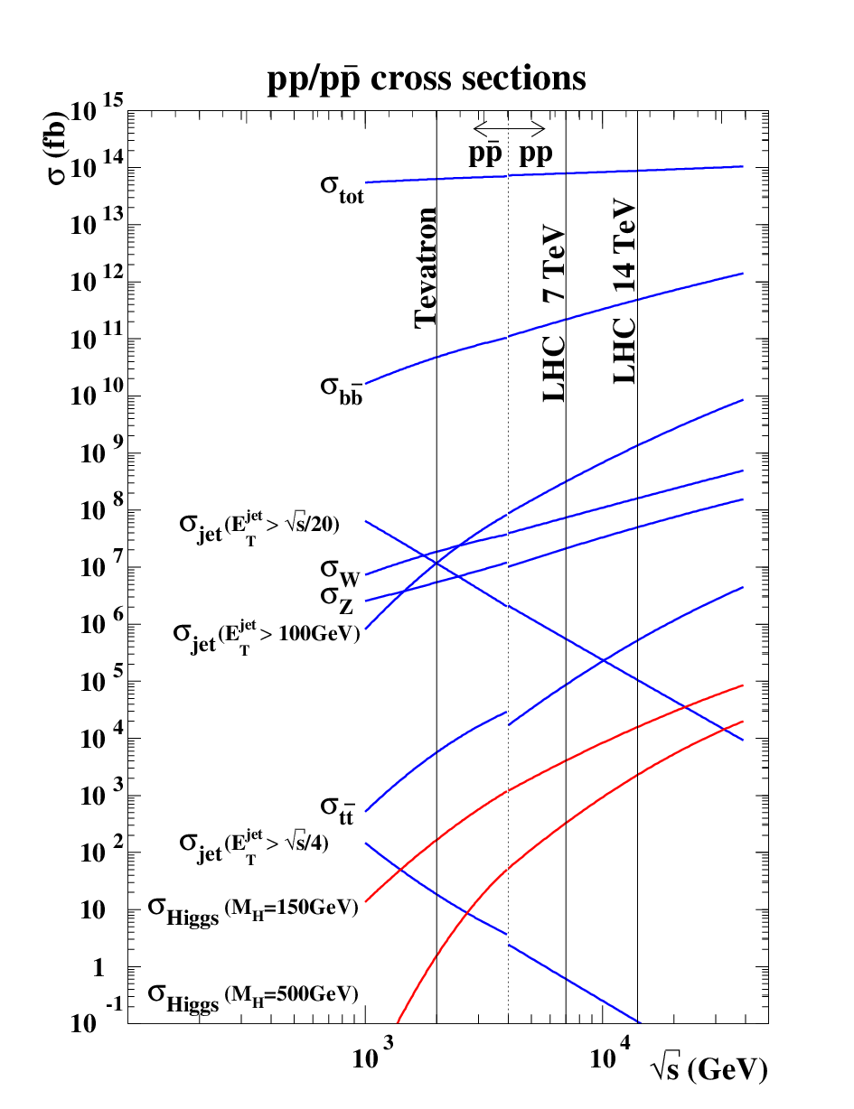
The combination of production mechanisms and decay modes of the Higgs boson and the particles that are eventually produced in association with the Higgs particle yields a plenitude of final-state topologies which can be used to search for Higgs-boson production. The following considerations have to be taken into account when choosing the most promising search channels: sufficient a priori signal rate determined by cross section and branching ratios, means to trigger on signal events with high efficiency, means to suppress the background to an acceptable level, means to estimate the uncertainties in the background prediction, and in the case of exclusion also the uncertainties in the signal prediction. It is desirable to be able to construct a final discriminating variable to distinguish the two alternative hypotheses of background-only and signal+background in addition to simple event counting. An obvious choice is the reconstructed mass of the Higgs-boson candidate events. Depending on the final-state particles this is not always possible. Alternatively or in addition other powerful observables can be used, e.g. the response of a multivariate event classifier.

For the discovery of a new resonance, which means that the probability to observe the actual number of events is less than $2.87\times 10^{-7}$ under the background-only hypothesis, only the background prediction and its uncertainty need to be known. Wrong assumptions on the shape of discriminating observables for the signal process will lead to a reduced sensitivity. Hypothetically one observed event can yield the claim of discovery given the search is basically background free ($\approx 3\times 10^{-7}$ expected background events) with vanishing systematic uncertainty, which unfortunately is never the case in the environments at colliders. For the exclusion of a signal hypothesis, neglecting systematic uncertainties and performing a counting-only experiment with negligible background, a minimal signal yield of 3 expected events after application of the full selection chain is needed in order to exclude the signal+background hypothesis at the 95% confidence level, when using the Bayesian or “CL_S” technique (see below). In this case the uncertainties on the signal rate and shape of the discriminating distributions will also influence the derived exclusion limits; for instance, a too optimistic assumption for the mass resolution for Higgs-boson candidates would yield a too stringent exclusion.

Although the Higgs mechanism had been incorporated in the electroweak theory in the late 1960s, it lasted until 1989, when LEP started its operation, before significant parts of the mass range of the SM Higgs boson could be investigated.⁶⁶ 6 A search carried out by the CDF experiment at Tevatron with up to $4.4\,\mathrm{pb^{-1}}$ at CM energy of 1.8 $\,\mathrm{TeV}$ excluded the mass ranges $2m_{\mu}{-}818\,\mathrm{MeV}$ and $846\,\mathrm{MeV}{-}2m_{\mathrm{K}}$ at 90% CL [93]. However, in this mass range the prediction of the branching ratios have large theoretical uncertainties, as discussed in Section 2.6. The particle data group in 1988 [94] concluded on Higgs-boson searches before the start of LEP “In summary, the only cast-iron constraint on the Higgs mass is $M_{\mathrm{H}}>14\,\mathrm{MeV}$. A combination of theoretical arguments and bounds from $B$, $\Upsilon$, and $K$ decays probably excludes the range below $4\,\mathrm{GeV}$.” Hence the mission of LEP was to probe the mass range of the SM Higgs boson starting from a zero mass to the highest possible mass values. For a discussion of Higgs-boson searches before the start of the LEP accelerator we, e.g., refer to Refs. [95, 96, 97, 98, 99]. In this article we review the most important results of the searches for the SM Higgs boson at the colliders LEP, Tevatron, and LHC. For details of the individual analyses, in particular identification criteria and systematic uncertainties, the original literature should be consulted.

References

- [1]
S. L. Glashow,
Nucl. Phys. 22 (1961) 579;
S. Weinberg, Phys. Rev. Lett. 19 (1967) 1264;
A. Salam, In the Proceedings of 8th Nobel Symposium, Lerum, Sweden, 19-25 May 1968, p. 367;
S. L. Glashow, J. Iliopoulos, L. Maiani, Phys. Rev. D 2 (1970) 1285. - [2]
Y. Nambu,
Phys. Rev. Lett. 4 (1960) 380;
J. Goldstone, Nuovo Cim. 19 (1961) 154;
J. Goldstone, A. Salam, S. Weinberg, Phys. Rev. 127 (1962) 965. - [3] F. Englert, R. Brout, Phys. Rev. Lett. 13 (1964) 321.
- [4] P. W. Higgs, Phys. Lett. 12 (1964) 132 and Phys. Rev. Lett. 13 (1964) 508.
- [5] G. S. Guralnik, C. R. Hagen, T. W. B. Kibble, Phys. Rev. Lett. 13 (1964) 585.
- [6]
D. J. Gross, F. Wilczek,
Phys. Rev. Lett. 30 (1973) 1343 and
Phys. Rev. D 8 (1973) 3633;
H. D. Politzer, Phys. Rev. Lett. 30 (1973) 1346;
H. Fritzsch, M. Gell-Mann, H. Leutwyler, Phys. Lett. B 47 (1973) 365;
H. Fritzsch, M. Gell-Mann, eConf C 720906V2 (1972) 135 [hep-ph/0208010]. - [7] G. ’t Hooft, M. J. G. Veltman, Nucl. Phys. B 50 (1972) 318.
- [8] B. W. Lee, J. Zinn-Justin, Phys. Rev. D 5 (1972) 3121, Phys. Rev. D 5 (1972) 3137 [Erratum-ibid. D 8 (1973) 4654] and Phys. Rev. D 7 (1973) 1049.
- [9] S. Weinberg, The Quantum Theory of Fields – Vol. 2: Modern Applications, Cambridge University Press, 1996.
- [10] M. Böhm, A. Denner, H. Joos, Gauge Theories of the Strong and Electroweak Interaction, B.G. Teubner Stuttgart/Leipzig/Wiesbaden, 2001.
- [11] G. Sterman, An Introduction to Quantum Field Theory, Cambridge University Press, 1993.
- [12] R.K. Ellis, W.J. Stirling, B.R. Webber, QCD and Collider Physics, Cambridge University Press, 1996.
- [13] J. Collins, Foundations of Perturbative QCD, Cambridge University Press, 2011.
- [14] D. A. Ross, M. J. G. Veltman, Nucl. Phys. B 95 (1975) 135.
- [15] [ALEPH, DELPHI, L3, OPAL and SLD Collaborations, LEP Electroweak Working Group and SLD Electroweak Group and SLD Heavy Flavour Group], Phys. Rept. 427 (2006) 257 [arXiv:hep-ex/0509008].
- [16] P. Sikivie, L. Susskind, M. B. Voloshin, V. I. Zakharov, Nucl. Phys. B 173 (1980) 189.
- [17] S. Dittmaier, M. Krämer, Phys. Rev. D 65 (2002) 073007 [hep-ph/0109062].
- [18] H. -L. Lai et al., Phys. Rev. D 82 (2010) 074024 [arXiv:1007.2241 [hep-ph]].
- [19] A. D. Martin, W. J. Stirling, R. S. Thorne, G. Watt, Eur. Phys. J. C 63 (2009) 189 [arXiv:0901.0002 [hep-ph]].
- [20] R. D. Ball et al., Nucl. Phys. B 849 (2011) 296 [arXiv:1101.1300 [hep-ph]].
- [21] S. Alekhin, J. Blümlein, S. Moch, Phys. Rev. D 86 (2012) 054009 [arXiv:1202.2281 [hep-ph]].
- [22] M. Glück, P. Jimenez-Delgado, E. Reya, C. Schuck, Phys. Lett. B 664 (2008) 133 [arXiv:0801.3618 [hep-ph]].
- [23] A. Cooper-Sarkar [for the H1 and ZEUS Collaboration], arXiv:1012.1438 [hep-ph].
- [24]
M. Botje et al.,
arXiv:1101.0538 [hep-ph];
PDF4LHC steering committee, http://www.hep.ucl.ac.uk/pdf4lhc/, 2010. - [25] S. Dittmaier, G. Passarino, C. Mariotti, R. Tanaka et al. [LHC Higgs Cross Section Working Group], CERN-2011-002, arXiv:1101.0593 [hep-ph].
- [26] S. Dittmaier, G. Passarino, C. Mariotti, R. Tanaka et al. [LHC Higgs Cross Section Working Group], CERN-2012-002, arXiv:1201.3084 [hep-ph].
- [27] A. D. Martin, R. G. Roberts, W. J. Stirling, R. S. Thorne, Eur. Phys. J. C 39 (2005) 155 [hep-ph/0411040].
- [28]
H. Spiesberger,
Phys. Rev. D 52 (1995) 4936
[hep-ph/9412286];
M. Roth, S. Weinzierl, Phys. Lett. B 590 (2004) 190 [hep-ph/0403200]. - [29] B. W. Lee, J. Zinn-Justin, Phys. Rev. D 5 (1972) 3155.
- [30]
T. Appelquist, C. W. Bernard,
Phys. Rev. D 22 (1980) 200;
A. C. Longhitano, Nucl. Phys. B 188 (1981) 118. - [31] J. M. Cornwall, D. N. Levin, G. Tiktopoulos, Phys. Rev. D 10 (1974) 1145 [Erratum-ibid. D 11 (1975) 972].
- [32]
M. J. Herrero, E. Ruiz Morales,
Nucl. Phys. B 418 (1994) 431
[hep-ph/9308276] and
Nucl. Phys. B 437 (1995) 319
[hep-ph/9411207];
D. Espriu, J. Matias, Phys. Lett. B 341 (1995) 332 [hep-ph/9407292];
S. Dittmaier, C. Grosse-Knetter, Nucl. Phys. B 459 (1996) 497 [hep-ph/9505266];
A. Nyffeler, A. Schenk, Phys. Rev. D 62 (2000) 113006 [hep-ph/9907294]. - [33]
J. van der Bij, M. J. G. Veltman,
Nucl. Phys. B 231 (1984) 205;
R. Barbieri, P. Ciafaloni, A. Strumia, Phys. Lett. B 317 (1993) 381. - [34] R. Boughezal, J. B. Tausk, J. J. van der Bij, Nucl. Phys. B 713 (2005) 278 [hep-ph/0410216].
- [35]
C. E. Vayonakis,
Lett. Nuovo Cim. 17 (1976) 383;
M. S. Chanowitz, M. K. Gaillard, Nucl. Phys. B 261 (1985) 379;
G. J. Gounaris, R. Kögerler, H. Neufeld, Phys. Rev. D 34 (1986) 3257. - [36]
Y. -P. Yao, C. P. Yuan,
Phys. Rev. D 38 (1988) 2237;
J. Bagger, C. Schmidt, Phys. Rev. D 41 (1990) 264;
H. -J. He, Y. -P. Kuang, X. -y. Li, Phys. Rev. Lett. 69 (1992) 2619 and Phys. Rev. D 49 (1994) 4842;
A. Denner, S. Dittmaier, Phys. Rev. D 54 (1996) 4499 [hep-ph/9603341]. - [37] C. Grosse-Knetter, Z. Phys. C 67 (1995) 261 [hep-ph/9405412].
- [38] B. W. Lee, C. Quigg, H. B. Thacker, Phys. Rev. D 16 (1977) 1519.
- [39] T. Hambye, K. Riesselmann, Phys. Rev. D 55 (1997) 7255 [hep-ph/9610272].
- [40]
L. Maiani, G. Parisi, R. Petronzio,
Nucl. Phys. B 136 (1978) 115;
M. Lindner, Z. Phys. C 31 (1986) 295. - [41]
Z. Fodor, K. Holland, J. Kuti, D. Nogradi, C. Schroeder,
PoS LAT 2007 (2007) 056
[arXiv:0710.3151 [hep-lat]];
P. Gerhold, K. Jansen, JHEP 0907 (2009) 025 [arXiv:0902.4135 [hep-lat]]. - [42] S. R. Coleman, E. J. Weinberg, Phys. Rev. D 7 (1973) 1888.
- [43]
M. Lindner, M. Sher, H. W. Zaglauer,
Phys. Lett. B 228 (1989) 139;
M. Sher, Phys. Rept. 179 (1989) 273;
G. Altarelli, G. Isidori, Phys. Lett. B 337 (1994) 141;
J. A. Casas, J. R. Espinosa, M. Quiros, Phys. Lett. B 342 (1995) 171 [hep-ph/9409458] and Phys. Lett. B 382 (1996) 374 [hep-ph/9603227]. - [44] J. Ellis et al., Phys. Lett. B 679 (2009) 369 [arXiv:0906.0954 [hep-ph]].
- [45] The LEP Electroweak Working Group, http://lepewwg.web.cern.ch/LEPEWWG/ .
- [46] M. Baak et al., Eur. Phys. J. C 72 (2012) 2205 [arXiv:1209.2716 [hep-ph]].
- [47] A. B. Arbuzov et al., Comput. Phys. Commun. 174 (2006) 728 [hep-ph/0507146].
- [48] G. Montagna, O. Nicrosini, F. Piccinini, G. Passarino, Comput. Phys. Commun. 117 (1999) 278 [hep-ph/9804211].
- [49] D. Bardin, G. Passarino, The Standard Model in the Making: Precision Study of the Electroweak Interactions Oxford University Press, 1999.
- [50] O. Eberhardt et al., Phys. Rev. Lett. 109 (2012) 241802 [arXiv:1209.1101 [hep-ph]].
- [51]
A. Djouadi, J. Kalinowski, M. Spira,
Comput. Phys. Commun. 108 (1998) 56
[arXiv:hep-ph/9704448];
A. Djouadi, J. Kalinowski, M. Mühlleitner, M. Spira, in Proceedings of 6th Les Houches Workshop: Physics at TeV Colliders, Les Houches, 2009, arXiv:1003.1643 [hep-ph]. - [52] A. Denner et al., Eur. Phys. J. C 71 (2011) 1753 [arXiv:1107.5909 [hep-ph]].
- [53] N. Kauer, G. Passarino, JHEP 1208 (2012) 116 [arXiv:1206.4803 [hep-ph]].
- [54]
G. Passarino, C. Sturm, S. Uccirati,
Nucl. Phys. B 834 (2010) 77
[arXiv:1001.3360 [hep-ph]];
S. Goria, G. Passarino, D. Rosco, Nucl. Phys. B 864 (2012) 530 [arXiv:1112.5517 [hep-ph]]. - [55] C. Anastasiou, S. Buehler, F. Herzog, A. Lazopoulos, JHEP 1204 (2012) 004 [arXiv:1202.3638 [hep-ph]].
- [56] L. Resnick, M. K. Sundaresan, P. J. S. Watson, Phys. Rev. D 8 (1973) 172.
- [57] J. R. Ellis, M. K. Gaillard, D. V. Nanopoulos, Nucl. Phys. B 106 (1976) 292.
- [58]
E. Braaten, J. P. Leveille,
Phys. Rev. D 22 (1980) 715;
N. Sakai, Phys. Rev. D 22 (1980) 2220;
T. Inami, T. Kubota, Nucl. Phys. B 179 (1981) 171;
M. Drees, K. -i. Hikasa, Phys. Lett. B 240 (1990) 455 [Erratum-ibid. B 262 (1991) 497]. - [59] M. Drees, K. -i. Hikasa, Phys. Rev. D 41 (1990) 1547.
- [60]
S. G. Gorishnii, A. L. Kataev, S. A. Larin,
Sov. J. Nucl. Phys. 40 (1984) 329
[Yad. Fiz. 40 (1984) 517];
S. G. Gorishnii, A. L. Kataev, S. A. Larin, L. R. Surguladze, Mod. Phys. Lett. A 5 (1990) 2703 and Phys. Rev. D 43 (1991) 1633;
L. R. Surguladze, Phys. Lett. B 341 (1994) 60 [hep-ph/9405325];
A. L. Kataev, V. T. Kim, Mod. Phys. Lett. A 9 (1994) 1309. K. G. Chetyrkin, A. Kwiatkowski, Nucl. Phys. B 461 (1996) 3 [hep-ph/9505358];
S. A. Larin, T. van Ritbergen, J. A. M. Vermaseren, Phys. Lett. B 362 (1995) 134 [hep-ph/9506465];
K. G. Chetyrkin, Phys. Lett. B 390 (1997) 309 [hep-ph/9608318];
K. G. Chetyrkin, M. Steinhauser, Phys. Lett. B 408 (1997) 320 [hep-ph/9706462];
P. A. Baikov, K. G. Chetyrkin, J. H. Kühn, Phys. Rev. Lett. 96 (2006) 012003 [hep-ph/0511063]. - [61] C. Anastasiou, F. Herzog, A. Lazopoulos, JHEP 1203 (2012) 035 [arXiv:1110.2368 [hep-ph]].
- [62] A. Djouadi, P. Gambino, Phys. Rev. D 51 (1995) 218 [Erratum-ibid. D 53 (1996) 4111] [hep-ph/9406431].
- [63]
K. Melnikov,
Phys. Rev. D 53 (1996) 5020
[hep-ph/9511310];
R. Harlander, M. Steinhauser, Phys. Rev. D 56 (1997) 3980 [hep-ph/9704436]. - [64] W. Bernreuther, A. Brandenburg, M. Flesch, Phys. Rev. D 56 (1997) 90 [hep-ph/9701347].
- [65] J. Fleischer, F. Jegerlehner, Phys. Rev. D 23 (1981) 2001.
- [66]
B. A. Kniehl,
Nucl. Phys. B 376 (1992) 3;
D. Y. .Bardin, B. M. Vilensky, P. K. Khristova, Sov. J. Nucl. Phys. 53 (1991) 152 [Yad. Fiz. 53 (1991) 240];
A. Dabelstein, W. Hollik, Z. Phys. C 53 (1992) 507. - [67]
Phys. Rev. D 50 (1994) 3314
[hep-ph/9405299];
A. Kwiatkowski, M. Steinhauser, Phys. Lett. B 338 (1994) 66 [Erratum-ibid. B 342 (1995) 455] [hep-ph/9405308];
A. Djouadi, P. Gambino, Phys. Rev. D 51 (1995) 218 [Erratum-ibid. D 53 (1996) 4111] [hep-ph/9406431];
B. A. Kniehl, M. Spira, Nucl. Phys. B 432 (1994) 39 [hep-ph/9410319]. B. A. Kniehl, M. Steinhauser, Phys. Lett. B 365 (1996) 297 [hep-ph/9507382] and , Nucl. Phys. B 454 (1995) 485 [hep-ph/9508241]. - [68]
A. Ghinculov,
Phys. Lett. B 337 (1994) 137
[Erratum-ibid. B 346 (1995) 426]
[hep-ph/9405394];
L. Durand, B. A. Kniehl, K. Riesselmann, Phys. Rev. D 51 (1995) 5007 [hep-ph/9412311]. - [69] A. Djouadi, Phys. Rept. 457 (2008) 1 [arXiv:hep-ph/0503172].
- [70] T. G. Rizzo, Phys. Rev. D 22 (1980) 178 [Addendum-ibid. D 22 (1980) 1824].
- [71]
T. Inami, T. Kubota, Y. Okada,
Z. Phys. C 18 (1983) 69;
A. Djouadi, M. Spira, P. M. Zerwas, Phys. Lett. B 264 (1991) 440. - [72] M. Spira, A. Djouadi, D. Graudenz, P. M. Zerwas, Nucl. Phys. B 453 (1995) 17 [hep-ph/9504378].
- [73]
K. G. Chetyrkin, B. A. Kniehl, M. Steinhauser,
Phys. Rev. Lett. 79 (1997) 353
[hep-ph/9705240] and
Nucl. Phys. B 510 (1998) 61
[hep-ph/9708255];
M. Schreck, M. Steinhauser, Phys. Lett. B 655 (2007) 148 [arXiv:0708.0916 [hep-ph]]. - [74] S. Actis, G. Passarino, C. Sturm, S. Uccirati, Phys. Lett. B 669 (2008) 62 [arXiv:0809.1302 [hep-ph]].
- [75] S. Actis, G. Passarino, C. Sturm, S. Uccirati, Nucl. Phys. B 811 (2009) 182 [arXiv:0809.3667 [hep-ph]].
- [76] M. Steinhauser, Phys. Rev. D 59 (1999) 054005 [hep-ph/9809507].
- [77] M. A. Shifman, A. I. Vainshtein, M. B. Voloshin, V. I. Zakharov, Sov. J. Nucl. Phys. 30 (1979) 711 [Yad. Fiz. 30 (1979) 1368].
- [78]
H.-Q. Zheng, D.-D. Wu,
Phys. Rev. D 42 (1990) 3760;
A. Djouadi, M. Spira, J. J. van der Bij, P. M. Zerwas, Phys. Lett. B 257 (1991) 187;
S. Dawson, R. P. Kauffman, Phys. Rev. D 47 (1993) 1264. - [79]
K. Melnikov, O. I. Yakovlev,
Phys. Lett. B 312 (1993) 179
[hep-ph/9302281];
M. Inoue, R. Najima, T. Oka, J. Saito, Mod. Phys. Lett. A 9 (1994) 1189;
J. Fleischer, O. V. Tarasov, V. O. Tarasov, Phys. Lett. B 584 (2004) 294 [hep-ph/0401090]. - [80] K. Melnikov, M. Spira, O. I. Yakovlev, Z. Phys. C 64 (1994) 401 [hep-ph/9405301].
- [81] U. Aglietti, R. Bonciani, G. Degrassi, A. Vicini, Phys. Lett. B 595 (2004) 432 [hep-ph/0404071].
- [82] M. Steinhauser, hep-ph/9612395.
- [83] M. Spira, A. Djouadi, P. M. Zerwas, Phys. Lett. B 276 (1992) 350.
- [84]
C. A. Nelson,
Phys. Rev. D 37 (1988) 1220;
A. Soni, R. M. Xu, Phys. Rev. D 48 (1993) 5259 [hep-ph/9301225];
D. Chang, W. Y. Keung, I. Phillips, Phys. Rev. D 48 (1993) 3225 [hep-ph/9303226];
A. Skjold, P. Osland, Phys. Lett. B 311 (1993) 261 [hep-ph/9303294];
V.D. Barger et al., Phys. Rev. D 49 (1994) 79 [hep-ph/9306270];
T. Arens, L. M. Sehgal, Z. Phys. C 66 (1995) 89 [hep-ph/9409396];
C. P. Buszello, I. Fleck, P. Marquard, J. J. van der Bij, Eur. Phys. J. C 32 (2004) 209 [hep-ph/0212396];
S. Y. Choi, D. J. Miller, M. M. Mühlleitner, P. M. Zerwas, Phys. Lett. B 553 (2003) 61 [hep-ph/0210077]. - [85]
B.A. Kniehl,
Nucl. Phys. B 352 (1991) 1 and
Nucl. Phys. B 357 (1991) 439;
D.Y. Bardin, P.K. Khristova, B.M. Vilensky, Sov. J. Nucl. Phys. 54 (1991) 833 [Yad. Fiz. 54 (1991) 1366]. - [86] A. Bredenstein, A. Denner, S. Dittmaier, M. M. Weber, Phys. Rev. D 74 (2006) 013004 [arXiv:hep-ph/0604011] and JHEP 0702 (2007) 080 [arXiv:hep-ph/0611234].
- [87]
Nucl. Phys. B 455 (1995) 21
[hep-ph/9507240];
A. Frink, B.A. Kniehl, D. Kreimer, K. Riesselmann, Phys. Rev. D 54 (1996) 4548 [hep-ph/9606310]. - [88]
A. Denner, S. Dittmaier, M. Roth, D. Wackeroth,
Nucl. Phys. B 560 (1999) 33
[arXiv:hep-ph/9904472];
A. Denner, S. Dittmaier, M. Roth, L. H. Wieders, Nucl. Phys. B 724 (2005) 247 [arXiv:hep-ph/0505042]. - [89] M. Spira, Fortsch. Phys. 46 (1998) 203 [arXiv:hep-ph/9705337].
- [90] J. Baglio, A. Djouadi, JHEP 1103 (2011) 055 [arXiv:1012.0530 [hep-ph]].
- [91] T. Sjöstrand, S. Mrenna, P. Z. Skands, JHEP 0605 (2006) 026 [hep-ph/0603175].
- [92] T. Sjöstrand, S. Mrenna, P. Z. Skands, Comput. Phys. Commun. 178 (2008) 852 [arXiv:0710.3820 [hep-ph]].
- [93] F. Abe et al. [CDF Collaboration], Phys. Rev. D 41 (1990) 1717.
- [94] G. P. Yost et al. [Particle Data Group Collaboration], Phys. Lett. B 204 (1988) 1.
- [95] A. S. Schwarz, Phys. Scripta 33 (1986) 5.
- [96] J. F. Gunion, H. E. Haber, G. L. Kane, S. Dawson, Front. Phys. 80 (2000) 1.
- [97] R. N. Cahn, Nucl. Phys. Proc. Suppl. 13 (1990) 155.
- [98] E. Gross, P. Yepes, Int. J. Mod. Phys. A 8 (1993) 407.
- [99] M. M. Kado, C. G. Tully, Ann. Rev. Nucl. Part. Sci. 52 (2002) 65.
- [100] C. Cowan. “Statistics” in J. Beringer et al. [Particle Data Group Collaboration], Phys. Rev. D 86 (2012) 010001.
- [101] G. Cowan, “Statistical Data analysis”, Oxford University Press (1997). [113]
- [102] O. Helene, Nucl. Instrum. Meth. 212 (1983) 319.
- [103] G. Zech, Nucl. Instrum. Meth. A 277 (1989) 608.
- [104]
V. F. Obraztsov,
Nucl. Instrum. Meth. A 4316 (1992) 388;
A. Favara, M. Pieri, hep-ex/9706016;
P. Bock, JHEP 0701 (2007) 080, [hep-ex/0405072]. - [105] J. Neyman and E. S.Pearson, Phil. Trans. R. Soc. Lond. A 231 (1933), 289.
- [106] A. L. Read, J. Phys. G G 28 (2002) 2693.
- [107] T. Junk, Nucl. Instrum. Meth. A 434 (1999) 435, [hep-ex/9902006].
- [108] R. D. Cousins, V. L. Highland, Nucl. Instrum. Meth. A 320 (1992) 331.
- [109] G. Cowan, K. Cranmer, E. Gross, O. Vitells, Eur. Phys. J. C 71 (2011) 1554, [arXiv:1007.1727 [physics.data-an]].
- [110] S. S. Wilks, Ann. Math. Statist. 9 (1938) 60.
- [111] A. Wald, Transactions of the American Mathematical Society, Vol. 54, No. 3 (1943), 426.
- [112] E. Gross, O. Vitells, Eur. Phys. J. C 70 (2010) 525 [arXiv:1005.1891 [physics.data-an]].
- [113] O. J. Dunn, J. Am. Statist. Assoc. 56 (1961) 52.
- [114] ATLAS Collaboration, CMS Collaboration and the LHC Higgs Combination Group, “Procedure for the LHC Higgs boson search combination in Summer 2011”, ATL-PHYS-PUB-2011-11, CMS NOTE-2011/005.
- [115] M. S. Carena et al., in Physics at LEP2, eds. G. Altarelli, T. Sjöstrand and F. Zwirner (CERN 96-01, Geneva, 1996), Vol. 1, p. 351, [hep-ph/9602250].
- [116] W. Kilian, M. Krämer, P. M. Zerwas, Phys. Lett. B 373 (1996) 135 [hep-ph/9512355].
- [117] F. Boudjema et al., eConf C 050318 (2005) 0601 [hep-ph/0510184].
- [118] W. Bernreuther et al., in Z Physics at LEP1, eds. G. Altarelli, R. Kleiss, C. Verzegnassi (CERN 89-08, Geneva, 1989), Vol. 2, p. 1.
- [119]
E. Accomando et al. [ECFA/DESY LC Physics Working Group Collaboration],
Phys. Rept. 299 (1998) 1
[hep-ph/9705442];
J. A. Aguilar-Saavedra et al. [ECFA/DESY LC Physics Working Group Collaboration], hep-ph/0106315;
T. Abe et al. [American Linear Collider Working Group Collaboration], hep-ex/0106056;
G. Aarons et al. [ILC Collaboration], arXiv:0709.1893 [hep-ph]. - [120] W. Beenakker et al., in Physics at LEP2 (Report CERN 96-01, Geneva, 1996), eds. A. Altarelli, T. Sjöstrand, F. Zwirner, Vol. 1, p.3, hep-ph/9602351.
- [121]
R. N. Cahn, M. S. Chanowitz, N. Fleishon,
Phys. Lett. B 82 (1979) 113;
L. Bergstrom, G. Hulth, Nucl. Phys. B 259 (1985) 137 [Erratum-ibid. B 276 (1986) 744];
A. Barroso, J. Pulido, J. C. Romao, Nucl. Phys. B 267 (1986) 509. - [122]
A. Abbasabadi, D. Bowser-Chao, D. A. Dicus, W. W. Repko,
Phys. Rev. D 52 (1995) 3919
[hep-ph/9507463];
A. Djouadi, V. Driesen, W. Hollik, J. Rosiek, Nucl. Phys. B 491 (1997) 68 [hep-ph/9609420]. - [123] D. R. T. Jones, S. T. Petcov, Phys. Lett. B 84 (1979) 440.
- [124]
J. Fleischer, F. Jegerlehner,
Nucl. Phys. B 216 (1983) 469;
B. A. Kniehl, Z. Phys. C 55 (1992) 605;
A. Denner, J. Küblbeck, R. Mertig, M. Böhm, Z. Phys. C 56 (1992) 261. - [125] F. Jegerlehner, K. Kolodziej, T. Westwanski, Eur. Phys. J. C 44 (2005) 195 [hep-ph/0503169].
- [126] S. Dawson, J. L. Rosner, Phys. Lett. B 148 (1984) 497.
- [127] K. -i. Hikasa, Phys. Lett. B 164 (1985) 385 [Erratum-ibid. 195B (1987) 623].
- [128] D. A. Dicus, S. S. D. Willenbrock, Phys. Rev. D 32 (1985) 1642.
- [129] G. Altarelli, B. Mele, F. Pitolli, Nucl. Phys. B 287 (1987) 205.
- [130] G. Belanger et al., Phys. Lett. B 559 (2003) 252 [hep-ph/0212261].
- [131] A. Denner, S. Dittmaier, M. Roth, M. M. Weber, Phys. Lett. B 560 (2003) 196 [hep-ph/0301189] and Nucl. Phys. B 660 (2003) 289 [hep-ph/0302198].
- [132] F. Boudjema et al., Phys. Lett. B 600 (2004) 65 [hep-ph/0407065].
- [133] A. Djouadi, J. Kalinowski, P. M. Zerwas, Z. Phys. C 54 (1992) 255.
- [134] J. F. Gunion, B. Grzadkowski, X. -G. He, Phys. Rev. Lett. 77 (1996) 5172 [hep-ph/9605326].
- [135]
H. Baer, S. Dawson, L. Reina,
Phys. Rev. D 61 (2000) 013002
[hep-ph/9906419];
A. Juste, G. Merino, hep-ph/9910301. - [136] M. Battaglia, K. Desch, AIP Conf. Proc. 578 (2001) 163 [hep-ph/0101165].
- [137]
S. Dittmaier et al.,
Phys. Lett. B 441 (1998) 383
[hep-ph/9808433];
S. Dawson, L. Reina, Phys. Rev. D 59 (1999) 054012 [arXiv:hep-ph/9808443]. - [138]
Y. You et al.,
Phys. Lett. B 571 (2003) 85
[hep-ph/0306036];
G. Belanger et al., Phys. Lett. B 571 (2003) 163 [hep-ph/0307029];
A. Denner, S. Dittmaier, M. Roth, M. M. Weber, Phys. Lett. B 575 (2003) 290 [hep-ph/0307193] and Nucl. Phys. B 680 (2004) 85 [hep-ph/0309274]. - [139] C. Farrell, A. H. Hoang, Phys. Rev. D 72 (2005) 014007 [hep-ph/0504220] and Phys. Rev. D 74 (2006) 014008 [hep-ph/0604166].
- [140]
S. Moretti,
Phys. Lett. B 452 (1999) 338
[hep-ph/9902214];
C. Schwinn, hep-ph/0412028;
K. Kolodziej, S. Szczypinski, Nucl. Phys. B 801 (2008) 153 [arXiv:0803.0887 [hep-ph]] and Eur. Phys. J. C 64 (2009) 645 [arXiv:0903.4606 [hep-ph]]. - [141] G. J. Gounaris, D. Schildknecht, F. M. Renard, Phys. Lett. B 83 (1979) 191.
- [142]
F. Boudjema, E. Chopin,
Z. Phys. C 73 (1996) 85
[hep-ph/9507396];
V. A. Ilyin et al., Phys. Rev. D 54 (1996) 6717 [hep-ph/9506326];
A. Djouadi, W. Kilian, M. Mühlleitner, P. M. Zerwas, Eur. Phys. J. C 10 (1999) 27 [hep-ph/9903229];
D. J. Miller, S. Moretti, Eur. Phys. J. C 13 (2000) 459 [hep-ph/9906395];
U. Baur, Phys. Rev. D 80 (2009) 013012 [arXiv:0906.0028 [hep-ph]]. - [143]
G. Belanger et al.,
Phys. Lett. B 576 (2003) 152
[hep-ph/0309010];
R. -Y. Zhang et al., Phys. Lett. B 578 (2004) 349 [hep-ph/0308203]. - [144] M. Davier, H. Nguyen Ngoc, Phys. Lett. B 229 (1989) 150.
- [145] G. Altarelli, R. Kleiss, C. Verzegnassi, (Eds.), CERN-89-08-V-2.
- [146] D. Decamp et al. [ALEPH Collaboration], Phys. Lett. B 236 (1990) 233.
- [147] P. Abreu et al. [DELPHI Collaboration], Nucl. Phys. B 342 (1990) 1.
- [148] B. Adeva et al. [L3 Collaboration], Phys. Lett. B 248 (1990) 203.
- [149] P. D. Acton et al. [OPAL Collaboration], Phys. Lett. B 268 (1991) 122.
- [150] D. Decamp et al. [ALEPH Collaboration], Phys. Lett. B 246 (1990) 306.
- [151] P. Abreu et al. [DELPHI Collaboration], Z. Phys. C 51 (1991) 25.
- [152] B. Adeva et al. [L3 Collaboration], Phys. Lett. B 252 (1990) 518.
- [153] M. Z. Akrawy et al. [OPAL Collaboration], Z. Phys. C 49 (1991) 1.
- [154] P. Abreu et al. [DELPHI Collaboration], Nucl. Phys. B 373 (1992) 3.
- [155] B. Adeva et al. [L3 Collaboration], Phys. Lett. B 283 (1992) 454.
- [156] M. Z. Akrawy et al. [OPAL Collaboration], Phys. Lett. B 253 (1991) 511.
- [157] D. Buskulic et al. [ALEPH Collaboration], Phys. Lett. B 384 (1996) 427.
- [158] P. Abreu et al. [DELPHI Collaboration], Nucl. Phys. B 421 (1994) 3.
- [159] M. Acciarri et al. [L3 Collaboration], Phys. Lett. B 385 (1996) 454.
- [160] G. Alexander et al. [OPAL Collaboration], Z. Phys. C 73 (1997) 189.
- [161] D. Decamp et al. [ALEPH Collaboration], Phys. Lett. B 241 (1990) 141.
- [162] D. Decamp et al. [ALEPH Collaboration], Phys. Lett. B 245 (1990) 289.
- [163] D. Decamp et al. [ALEPH Collaboration], Phys. Rept. 216 (1992) 253.
- [164] D. Buskulic et al. [ALEPH Collaboration], Phys. Lett. B 313 (1993) 299.
- [165] B. Adeva et al. [L3 Collaboration], Phys. Lett. B 257 (1991) 450.
- [166] O. Adriani et al. [L3 Collaboration], Phys. Lett. B 303 (1993) 391.
- [167] M. Z. Akrawy et al. [OPAL Collaboration], Phys. Lett. B 236 (1990) 224.
- [168] M. Z. Akrawy et al. [OPAL Collaboration], Phys. Lett. B 251 (1990) 211.
- [169] R. Akers et al. [OPAL Collaboration], Phys. Lett. B 327 (1994) 397.
- [170] J. F. Grivaz, F. Le Diberder, Nucl. Instrum. Meth. A 333 (1993) 320;
- [171] R. Barate et al. [ALEPH Collaboration], Phys. Lett. B 412 (1997) 155.
- [172] R. Barate et al. [ALEPH Collaboration], Phys. Lett. B 495 (2000) 1 [hep-ex/0011045].
- [173] P. Janot “HZHA”, in Physics at LEP2, eds. G. Altarelli, T. Sjöstrand and F. Zwirner (CERN 96-01, Geneva, 1996), Vol. 2, p. 299, [hep-ph/9602203].
- [174] K. Ackerstaff et al. [OPAL Collaboration], Phys. Lett. B 393 (1997) 231.
- [175] P. Abreu et al. [DELPHI Collaboration], Eur. Phys. J. C 2 (1998) 1.
- [176] M. Acciarri et al. [L3 Collaboration], Phys. Lett. B 411 (1997) 373.
- [177] K. Ackerstaff et al. [OPAL Collaboration], Eur. Phys. J. C 1 (1998) 425 [hep-ex/9709003].
- [178] R. Barate et al. [ALEPH Collaboration], Phys. Lett. B 440 (1998) 403 [Phys. Lett. B 447 (1999) 336] [hep-ex/9811032].
- [179] P. Abreu et al. [DELPHI Collaboration], Eur. Phys. J. C 10 (1999) 563.
- [180] M. Acciarri et al. [L3 Collaboration], Phys. Lett. B 431 (1998) 437.
- [181] G. Abbiendi et al. [OPAL Collaboration], Eur. Phys. J. C 7 (1999) 407 [hep-ex/9811025].
- [182] R. Barate et al. [ALEPH Collaboration], Eur. Phys. J. C 17 (2000) 223.
- [183] P. Abreu et al. [DELPHI Collaboration], Eur. Phys. J. C 17 (2000) 187 [Addendum-ibid. C 17 (2000) 549] [hep-ex/0104020].
- [184] M. Acciarri et al. [L3 Collaboration], Phys. Lett. B 461 (1999) 376 [hep-ex/9909004].
- [185] G. Abbiendi et al. [OPAL Collaboration], Eur. Phys. J. C 12 (2000) 567 [hep-ex/9908002].
- [186] R. Barate et al. [ALEPH Collaboration], Phys. Lett. B 499 (2001) 53 [hep-ex/0010062].
- [187] J. Abdallah et al. [DELPHI Collaboration], Eur. Phys. J. C 23 (2002) 409 [hep-ex/0201022].
- [188] M. Acciarri et al. [L3 Collaboration], Phys. Lett. B 508 (2001) 225 [hep-ex/0012019].
- [189] P. Abreu et al. [DELPHI Collaboration], Phys. Lett. B 499 (2001) 23 [hep-ex/0102036].
- [190] G. Abbiendi et al. [OPAL Collaboration], Phys. Lett. B 499 (2001) 38 [hep-ex/0101014].
- [191] A. Heister et al. [ALEPH Collaboration], Phys. Lett. B 526 (2002) 191 [hep-ex/0201014].
- [192] J. Abdallah et al. [DELPHI Collaboration], Eur. Phys. J. C 32 (2004) 145 [hep-ex/0303013].
- [193] P. Achard et al. [L3 Collaboration], Phys. Lett. B 517 (2001) 319 [hep-ex/0107054].
- [194] G. Abbiendi et al. [OPAL Collaboration], Eur. Phys. J. C 26 (2003) 479 [hep-ex/0209078].
- [195] S. Jin,Peter McNamara, Nucl. Instrum. Meth. A 462 (2001) 561.
- [196] M. Acciarri et al. [L3 Collaboration], Phys. Lett. B 495 (2000) 18 [hep-ex/0011043].
- [197] R. Barate et al. [ALEPH and DELPHI and L3 and OPAL Collaborations and LEP Working Group for Higgs boson searches], Phys. Lett. B 565 (2003) 61 [hep-ex/0306033].
- [198] U. Aglietti et al., hep-ph/0612172.
- [199]
J. Baglio, A. Djouadi,
JHEP 1010 (2010) 064
[arXiv:1003.4266 [hep-ph], arXiv:1009.1363 [hep-ph]];
J. Baglio, A. Djouadi, S. Ferrag, R. M. Godbole, Phys. Lett. B 699 (2011) 368 [Erratum-ibid. B 702 (2011) 105] [arXiv:1101.1832 [hep-ph]];
J. Baglio, A. Djouadi, R. Godbole, arXiv:1107.0281 [hep-ph]. - [200]
J. M. Butterworth, A. R. Davison, M. Rubin, G. P. Salam,
Phys. Rev. Lett. 100 (2008) 242001.
[arXiv:0802.2470 [hep-ph]];
J. M. Butterworth et al., ATL-PHYS-PUB-2009-088. - [201] T. Plehn, G. P. Salam, M. Spannowsky, Phys. Rev. Lett. 104 (2010) 111801 [arXiv:0910.5472 [hep-ph]].
- [202] H. M. Georgi, S. L. Glashow, M. E. Machacek, D. V. Nanopoulos, Phys. Rev. Lett. 40 (1978) 692.
- [203] D. Graudenz, M. Spira, P. M. Zerwas, Phys. Rev. Lett. 70 (1993) 1372.
- [204]
R. V. Harlander,
Phys. Lett. B 492 (2000) 74
[hep-ph/0007289];
S. Catani, D. de Florian, M. Grazzini, JHEP 0105 (2001) 025 [hep-ph/0102227];
R. V. Harlander, W. B. Kilgore, Phys. Rev. D 64 (2001) 013015 [hep-ph/0102241] and Phys. Rev. Lett. 88 (2002) 201801 [hep-ph/0201206];
C. Anastasiou, K. Melnikov, Nucl. Phys. B 646 (2002) 220 [hep-ph/0207004];
V. Ravindran, J. Smith, W. L. van Neerven, Nucl. Phys. B 665 (2003) 325 [hep-ph/0302135];
J. Blümlein, V. Ravindran, Nucl. Phys. B 716 (2005) 128 [hep-ph/0501178]. - [205]
S. Marzani et al.,
Nucl. Phys. B 800 (2008) 127
[arXiv:0801.2544 [hep-ph]];
R. V. Harlander, K. J. Ozeren, Phys. Lett. B 679 (2009) 467 [arXiv:0907.2997 [hep-ph]] and JHEP 0911 (2009) 088 [arXiv:0909.3420 [hep-ph]];
R. V. Harlander, H. Mantler, S. Marzani, K. J. Ozeren, Eur. Phys. J. C 66 (2010) 359 [arXiv:0912.2104 [hep-ph]];
A. Pak, M. Rogal, M. Steinhauser, Phys. Lett. B 679 (2009) 473 [arXiv:0907.2998 [hep-ph]] and JHEP 1002 (2010) 025 [arXiv:0911.4662 [hep-ph]]. - [206]
S. Catani, D. de Florian, M. Grazzini, P. Nason,
JHEP 0307 (2003) 028
[hep-ph/0306211];
S. Moch, A. Vogt, Phys. Lett. B 631 (2005) 48 [hep-ph/0508265];
E. Laenen, L. Magnea, Phys. Lett. B 632 (2006) 270 [hep-ph/0508284];
A. Idilbi, X. -d. Ji, J. -P. Ma, F. Yuan, Phys. Rev. D 73 (2006) 077501 [hep-ph/0509294];
V. Ravindran, Nucl. Phys. B 746 (2006) 58 [hep-ph/0512249]. - [207] V. Ahrens, T. Becher, M. Neubert, L. L. Yang, Phys. Rev. D 79 (2009) 033013 [arXiv:0808.3008 [hep-ph]], Eur. Phys. J. C 62 (2009) 333 [arXiv:0809.4283 [hep-ph]] and Phys. Lett. B 698 (2011) 271 [arXiv:1008.3162 [hep-ph]].
- [208] G. Degrassi, F. Maltoni, Phys. Lett. B 600 (2004) 255 [hep-ph/0407249].
- [209] S. Actis, G. Passarino, C. Sturm, S. Uccirati, Phys. Lett. B 670 (2008) 12 [arXiv:0809.1301 [hep-ph]].
- [210] C. Anastasiou, R. Boughezal, F. Petriello, JHEP 0904 (2009) 003 [arXiv:0811.3458 [hep-ph]].
- [211]
W. -Y. Keung, F. J. Petriello,
Phys. Rev. D 80 (2009) 013007
[arXiv:0905.2775 [hep-ph]];
O. Brein, Phys. Rev. D 81 (2010) 093006 [arXiv:1003.4438 [hep-ph]]. - [212]
E. Accomando,
Phys. Lett. B 661 (2008) 129
[arXiv:0709.1364 [hep-ph]];
T. Binoth, M. Ciccolini, N. Kauer, M. Krämer, JHEP 0612 (2006) 046 [hep-ph/0611170];
J. M. Campbell, R. K. Ellis, C. Williams, JHEP 1110 (2011) 005 [arXiv:1107.5569 [hep-ph]];
G. Passarino, JHEP 1208 (2012) 146 [arXiv:1206.3824 [hep-ph]]. - [213] D. de Florian, M. Grazzini, Phys. Lett. B 674 (2009) 291 [arXiv:0901.2427 [hep-ph]].
- [214]
D. de Florian, M. Grazzini, Z. Kunszt,
Phys. Rev. Lett. 82 (1999) 5209
[hep-ph/9902483];
V. Ravindran, J. Smith, W. L. Van Neerven, Nucl. Phys. B 634 (2002) 247 [hep-ph/0201114];
C. J. Glosser, C. R. Schmidt, JHEP 0212 (2002) 016 [hep-ph/0209248]. - [215] G. Bozzi, S. Catani, D. de Florian, M. Grazzini, Nucl. Phys. B 737 (2006) 73 [hep-ph/0508068]. Q. -H. Cao, C. -R. Chen, C. Schmidt, C. -P. Yuan, arXiv:0909.2305 [hep-ph].
- [216] D. de Florian, G. Ferrera, M. Grazzini, D. Tommasini, JHEP 1111 (2011) 064 [arXiv:1109.2109 [hep-ph]].
- [217]
C. F. Berger et al.,
JHEP 1104 (2011) 092
[arXiv:1012.4480 [hep-ph]];
I. W. Stewart, F. J. Tackmann, Phys. Rev. D 85 (2012) 034011 [arXiv:1107.2117 [hep-ph]];
T. Becher, M. Neubert, JHEP 1207 (2012) 108 [arXiv:1205.3806 [hep-ph]];
X. Liu, F. Petriello, arXiv:1210.1906 [hep-ph]. - [218]
C. Anastasiou, K. Melnikov, F. Petriello,
Phys. Rev. Lett. 93 (2004) 262002
[hep-ph/0409088] and
Nucl. Phys. B 724 (2005) 197
[hep-ph/0501130];
C. Anastasiou, G. Dissertori, F. Stöckli, JHEP 0709 (2007) 018 [arXiv:0707.2373 [hep-ph]]. - [219]
S. Catani, M. Grazzini,
Phys. Rev. Lett. 98 (2007) 222002
[hep-ph/0703012];
M. Grazzini, JHEP 0802 (2008) 043 [arXiv:0801.3232 [hep-ph]]. - [220] C. Anastasiou, S. Buehler, F. Herzog, A. Lazopoulos, JHEP 1112 (2011) 058 [arXiv:1107.0683 [hep-ph]].
- [221] D. de Florian, G. Ferrera, M. Grazzini, D. Tommasini, JHEP 1206 (2012) 132 [arXiv:1203.6321 [hep-ph]].
- [222] J. Campbell, K. Ellis, MCFM, http://mcfm.fnal.gov, 2010.
- [223]
C. F. Berger, V. Del Duca, L. J. Dixon,
Phys. Rev. D 74 (2006) 094021
[Erratum-ibid. D 76 (2007) 099901]
[hep-ph/0608180];
S. D. Badger, E. W. N. Glover, K. Risager, JHEP 0707 (2007) 066 [arXiv:0704.3914 [hep-ph]];
E. W. N. Glover, P. Mastrolia, C. Williams, JHEP 0808 (2008) 017 [arXiv:0804.4149 [hep-ph]];
S. Badger, E. W. N. Glover, P. Mastrolia, C. Williams, JHEP 1001 (2010) 036 [arXiv:0909.4475 [hep-ph]];
L. J. Dixon, Y. Sofianatos, JHEP 0908 (2009) 058 [arXiv:0906.0008 [hep-ph]];
S. Badger, J. M. Campbell, R. K. Ellis, C. Williams, JHEP 0912 (2009) 035 [arXiv:0910.4481 [hep-ph]]. - [224]
J. M. Campbell, R. K. Ellis, G. Zanderighi,
JHEP 0610 (2006) 028
[hep-ph/0608194];
J. M. Campbell, R. K. Ellis, C. Williams, Phys. Rev. D 81 (2010) 074023 [arXiv:1001.4495 [hep-ph]]. - [225] S. Frixione, B. R. Webber, JHEP 0206 (2002) 029 [hep-ph/0204244].
- [226] E. Bagnaschi, G. Degrassi, P. Slavich, A. Vicini, JHEP 1202 (2012) 088 [arXiv:1111.2854 [hep-ph]].
- [227]
A. Banfi, G. P. Salam, G. Zanderighi,
JHEP 1206 (2012) 159
[arXiv:1203.5773 [hep-ph]];
A. Banfi, P. F. Monni, G. P. Salam, G. Zanderighi, Phys. Rev. Lett. 109 (2012) 202001 [arXiv:1206.4998 [hep-ph]]. - [228] R. N. Cahn, S. Dawson, Phys. Lett. B 136 (1984) 196 [Erratum-ibid. B 138 (1984) 464].
- [229]
V. D. Barger, R. J. N. Phillips, D. Zeppenfeld,
Phys. Lett. B 346 (1995) 106
[hep-ph/9412276];
D. L. Rainwater, D. Zeppenfeld, JHEP 9712 (1997) 005 [hep-ph/9712271] and Phys. Rev. D 60 (1999) 113004 [Erratum-ibid. D 61 (2000) 099901] [hep-ph/9906218];
D. L. Rainwater, D. Zeppenfeld, K. Hagiwara, Phys. Rev. D 59 (1998) 014037 [hep-ph/9808468];
V. Del Duca et al., JHEP 0610 (2006) 016 [hep-ph/0608158]. - [230] V. Del Duca et al., Nucl. Phys. B 616 (2001) 367 [hep-ph/0108030].
- [231] A. Nikitenko, M. L. Vazquez Acosta, arXiv:0705.3585 [hep-ph].
- [232] T. Han, G. Valencia, S. Willenbrock, Phys. Rev. Lett. 69 (1992) 3274 [hep-ph/9206246].
- [233]
T. Figy, C. Oleari, D. Zeppenfeld,
Phys. Rev. D 68 (2003) 073005
[hep-ph/0306109];
T. Figy, D. Zeppenfeld, Phys. Lett. B 591 (2004) 297 [hep-ph/0403297]. - [234] M. Ciccolini, A. Denner, S. Dittmaier, Phys. Rev. Lett. 99 (2007) 161803 [arXiv:0707.0381 [hep-ph]] and Phys. Rev. D 77 (2008) 013002 [arXiv:0710.4749 [hep-ph]].
- [235] R. V. Harlander, J. Vollinga, M. M. Weber, Phys. Rev. D 77 (2008) 053010 [arXiv:0801.3355 [hep-ph]].
- [236] P. Bolzoni, F. Maltoni, S. -O. Moch, M. Zaro, Phys. Rev. Lett. 105 (2010) 011801 [arXiv:1003.4451 [hep-ph]].
- [237] P. Bolzoni, F. Maltoni, S. -O. Moch, M. Zaro, Phys. Rev. D 85 (2012) 035002 [arXiv:1109.3717 [hep-ph]].
- [238]
J. R. Andersen, T. Binoth, G. Heinrich, J. M. Smillie,
JHEP 0802 (2008) 057
[arXiv:0709.3513 [hep-ph]];
A. Bredenstein, K. Hagiwara, B. Jäger, Phys. Rev. D 77 (2008) 073004 [arXiv:0801.4231 [hep-ph]]. - [239] P. Nason, C. Oleari, JHEP 1002 (2010) 037 [arXiv:0911.5299 [hep-ph]].
- [240] T. Figy, S. Palmer, G. Weiglein, JHEP 1202 (2012) 105 [arXiv:1012.4789 [hep-ph]].
- [241] K. Arnold et al., VBFNLO, http://www-itp.particle.uni-karlsruhe.de/ vbfnloweb, 2009.
- [242]
A. Denner, S. Dittmaier, S. Kallweit, A. Mück, Hawk,
http://omnibus.uni-freiburg.de/sd565/programs/hawk/hawk.html, 2010. - [243]
P. Bolzoni, F. Maltoni, S. Moch, M. Zaro, VBF@NNLO,
http://vbf-nnlo.phys.ucl.ac.be/vbf.html, 2011. - [244]
S. L. Glashow, D. V. Nanopoulos, A. Yildiz,
Phys. Rev. D 18 (1978) 1724;
J. Finjord, G. Girardi, P. Sorba, Phys. Lett. B 89 (1979) 99. - [245]
T. Han, S. Willenbrock,
Phys. Lett. B273 (1991) 167;
H. Baer, B. Bailey, J. F. Owens, Phys. Rev. D47 (1993) 2730;
J. Ohnemus, W. J. Stirling, Phys. Rev. D47 (1993) 2722. - [246] O. Brein, A. Djouadi, R. Harlander, Phys. Lett. B579 (2004) 149 [hep-ph/0307206].
- [247] G. Ferrera, M. Grazzini, F. Tramontano, Phys. Rev. Lett. 107 (2011) 152003 [arXiv:1107.1164 [hep-ph]].
- [248] L. Altenkamp et al., JHEP 1302 (2013) 078 [arXiv:1211.5015 [hep-ph]].
- [249] O. Brein, R. Harlander, M. Wiesemann, T. Zirke, Eur. Phys. J. C 72 (2012) 1868 [arXiv:1111.0761 [hep-ph]].
- [250] M. L. Ciccolini, S. Dittmaier, M. Krämer, Phys. Rev. D68 (2003) 073003 [hep-ph/0306234].
- [251] A. Denner, S. Dittmaier, S. Kallweit, A. Mück, JHEP 1203 (2012) 075 [arXiv:1112.5142 [hep-ph]].
- [252] A. Banfi, J. Cancino, Phys. Lett. B 718 (2012) 499 [arXiv:1207.0674 [hep-ph]].
- [253] O. Brein, R. V. Harlander, T. J. E. Zirke, Comput. Phys. Commun. 184 (2013) 998 [arXiv:1210.5347 [hep-ph]].
- [254] M. Spira, V2HV, http://people.web.psi.ch/spira/v2hv, 2007.
- [255]
R. Raitio, W. W. Wada,
Phys. Rev. D 19 (1979) 941;
Z. Kunszt, Nucl. Phys. B 247 (1984) 339;
J. N. Ng, P. Zakarauskas, Phys. Rev. D 29 (1984) 876. - [256]
W. Beenakker et al.,
Phys. Rev. Lett. 87 (2001) 201805
[hep-ph/0107081] and
Nucl. Phys. B 653 (2003) 151
[hep-ph/0211352];
L. Reina, S. Dawson, Phys. Rev. Lett. 87 (2001) 201804 [arXiv:hep-ph/0107101];
L. Reina, S. Dawson, D. Wackeroth, Phys. Rev. D 65 (2002) 053017 [arXiv:hep-ph/0109066];
S. Dawson, L. H. Orr, L. Reina, D. Wackeroth, Phys. Rev. D 67 (2003) 071503 [arXiv:hep-ph/0211438];
S. Dawson et al., Phys. Rev. D 68 (2003) 034022 [arXiv:hep-ph/0305087]. - [257] R. Frederix et al., Phys. Lett. B 701 (2011) 427 [arXiv:1104.5613 [hep-ph]].
- [258] M. V. Garzelli, A. Kardos, C. G. Papadopoulos, Z. Trocsanyi, Europhys. Lett. 96 (2011) 11001 [arXiv:1108.0387 [hep-ph]].
- [259]
A. Bredenstein, A. Denner, S. Dittmaier, S. Pozzorini,
JHEP 0808 (2008) 108
[arXiv:0807.1248 [hep-ph]],
Phys. Rev. Lett. 103 (2009) 012002
[arXiv:0905.0110 [hep-ph]] and
JHEP 1003 (2010) 021
[arXiv:1001.4006 [hep-ph]];
G. Bevilacqua et al., JHEP 0909 (2009) 109 [arXiv:0907.4723 [hep-ph]]. - [260] G. Bevilacqua, M. Czakon, C. G. Papadopoulos, M. Worek, Phys. Rev. Lett. 104 (2010) 162002 [arXiv:1002.4009 [hep-ph]] and Phys. Rev. D 84 (2011) 114017 [arXiv:1108.2851 [hep-ph]].
- [261] M. Dührssen et al., Phys. Rev. D 70 (2004) 113009 [hep-ph/0406323].
- [262] ATLAS Collaboration, ATL-PHYS-PUB-2012-004.
- [263] CMS Collaboration, CMS-NOTE-2012-006.
- [264] R. Lafaye it et al., JHEP 0908 (2009) 009 [arXiv:0904.3866 [hep-ph]].
- [265] ATLAS Collaboration, ATLAS-CONF-2012-127.
- [266] CMS Collaboration, CMS PAS HIG-12-045.
- [267] LHC Higgs Cross Section Working Group, A. David et al., arXiv:1209.0040 [hep-ph].
- [268] G. Passarino, Nucl. Phys. B 868 (2013) 416 [arXiv:1209.5538 [hep-ph]].
- [269]
E. W. N. Glover, J. J. van der Bij,
Nucl. Phys. B 309 (1988) 282;
D. A. Dicus, C. Kao, S. S. D. Willenbrock, Phys. Lett. B 203 (1988) 457;
T. Plehn, M. Spira, P. M. Zerwas, Nucl. Phys. B 479 (1996) 46 [Erratum-ibid. B 531 (1998) 655] [hep-ph/9603205]. - [270] S. Dawson, S. Dittmaier, M. Spira, Phys. Rev. D 58 (1998) 115012 [hep-ph/9805244].
- [271]
V. D. Barger, T. Han, R. J. N. Phillips,
Phys. Rev. D 38 (1988) 2766;
M. Moretti et a;., JHEP 1011 (2010) 097 [arXiv:1008.0820 [hep-ph]]. - [272] A. Djouadi, W. Kilian, M. Mühlleitner, P. M. Zerwas, Eur. Phys. J. C 10 (1999) 45 [hep-ph/9904287].
- [273]
W. -Y. Keung,
Mod. Phys. Lett. A 2 (1987) 765;
O. J. P. Eboli, G. C. Marques, S. F. Novaes, A. A. Natale, Phys. Lett. B 197 (1987) 269;
D. A. Dicus, K. J. Kallianpur, S. S. D. Willenbrock, Phys. Lett. B 200 (1988) 187;
A. Abbasabadi, W. W. Repko, D. A. Dicus, R. Vega, Phys. Lett. B 213 (1988) 386. - [274] T. Figy, Mod. Phys. Lett. A 23 (2008) 1961 [arXiv:0806.2200 [hep-ph]].
- [275] U. Baur, T. Plehn, D. L. Rainwater, Phys. Rev. D 67 (2003) 033003 [hep-ph/0211224].
- [276] U. Baur, T. Plehn, D. L. Rainwater, Phys. Rev. D 69 (2004) 053004 [hep-ph/0310056].
- [277]
T. Plehn, M. Rauch,
Phys. Rev. D 72 (2005) 053008
[hep-ph/0507321];
T. Binoth, S. Karg, N. Kauer, R. Rückl, Phys. Rev. D 74 (2006) 113008 [hep-ph/0608057]. - [278] T. Aaltonen et al. [CDF Collaboration], JHEP 1302 (2013) 004 [arXiv:1208.6445 [hep-ex]].
- [279] Tevatron New Physics Higgs Working Group and CDF and D0 Collaborations, arXiv:1207.0449 [hep-ex].
- [280] T. Aaltonen et al. [CDF Collaboration], Phys. Lett. B 717 (2012) 173 [arXiv:1207.6386 [hep-ex]].
- [281] V. M. Abazov et al. [D0 Collaboration], Phys. Rev. Lett. 107 (2011) 151801 [arXiv:1107.4587 [hep-ex]].
- [282] T. Aaltonen et al. [CDF Collaboration], Phys. Rev. D 86 (2012) 072012 [arXiv:1207.5016 [hep-ex]].
- [283] T. Aaltonen et al. [CDF Collaboration], Phys. Rev. Lett. 109 (2012) 181802 [arXiv:1208.2662 [hep-ex]].
- [284] T. Aaltonen et al. [CDF Collaboration], Phys. Rev. Lett. 108 (2012) 181804 [arXiv:1201.4880 [hep-ex]].
- [285] V. M. Abazov et al. [D0 Collaboration], Phys. Lett. B 714 (2012) 237 [arXiv:1203.4443 [hep-ex]].
- [286] V. M. Abazov et al. [D0 Collaboration], Phys. Rev. Lett. 106 (2011) 171802 [arXiv:1101.6079 [hep-ex]].
- [287] T. Aaltonen et al. [CDF Collaboration], Phys. Rev. Lett. 104 (2010) 061803, [arXiv:1001.4468 [hep-ex]].
- [288] V. M. Abazov et al. [D0 Collaboration], Phys. Rev. D 84 (2011) 092002 [arXiv:1107.1268 [hep-ex]].
- [289] M. L. Mangano et al., JHEP 0307 (2003) 001 [hep-ph/0206293].
- [290] E. Boos et al. [CompHEP Collaboration], Nucl. Instrum. Meth. A 534 (2004) 250 [hep-ph/0403113].
- [291] G. Corcella et al., JHEP 0101 (2001) 010 [hep-ph/0011363].
- [292] M. Bahr et al., Eur. Phys. J. C 58 (2008) 639 [arXiv:0803.0883 [hep-ph]].
- [293] S. Frixione et al., arXiv:1010.0819 [hep-ph].
- [294] T. Gleisberg et al., JHEP 0902 (2009) 007 [arXiv:0811.4622 [hep-ph]].
- [295] T. Aaltonen et al. [CDF Collaboration], Phys. Rev. Lett. 109 (2012) 111804 [arXiv:1207.1703 [hep-ex]].
- [296] V. M. Abazov et al. [D0 Collaboration], Phys. Rev. Lett. 109 (2012) 121804 [arXiv:1208.0653 [hep-ex]].
- [297] T. Aaltonen et al. [CDF Collaboration], Phys. Rev. Lett. 109 (2012) 111805 [arXiv:1207.1711 [hep-ex]].
- [298] V. M. Abazov et al. [D0 Collaboration], Phys. Lett. B 716 (2012) 285 [arXiv:1207.5689 [hep-ex]].
- [299] T. Aaltonen et al. [CDF Collaboration], Phys. Rev. Lett. 109 (2012) 111803 [arXiv:1207.1704 [hep-ex]].
- [300] V. M. Abazov et al. [D0 Collaboration], Phys. Rev. Lett. 109 (2012) 121803 [arXiv:1207.5819 [hep-ex]].
- [301] V. M. Abazov et al. [D0 Collaboration], Phys. Rev. Lett. 109 (2012) 121802 [arXiv:1207.6631 [hep-ex]].
- [302] T. Aaltonen et al. [CDF Collaboration], Phys. Rev. Lett. 109 (2012) 111802 [arXiv:1207.1707 [hep-ex]].
- [303] T. Aaltonen et al. [CDF and D0 Collaborations], Phys. Rev. Lett. 109 (2012) 071804, [arXiv:1207.6436 [hep-ex]].
- [304] M. Dittmar, H. K. Dreiner, Phys. Rev. D 55 (1997) 167 [hep-ph/9608317].
- [305] T. Aaltonen et al. [CDF and D0 Collaborations], Phys. Rev. Lett. 104 (2010) 061802 [arXiv:1001.4162 [hep-ex]].
- [306] V. M. Abazov et al. [D0 Collaboration],
- [307] V. M. Abazov et al. [D0 Collaboration], Phys. Rev. D 86 (2012) 032010 [arXiv:1207.1041 [hep-ex]].
- [308]
The LHC Higgs Cross Section Working Group,
https://twiki.cern.ch/twiki/bin/view/LHCPhysics/CrossSections . - [309] J. Alwall et al., JHEP 1106 (2011) 128 [arXiv:1106.0522 [hep-ph]].
- [310] T. Binoth, M. Ciccolini, N. Kauer, M. Krämer, JHEP 0503 (2005) 065 [hep-ph/0503094].
- [311] T. Binoth, N. Kauer, P. Mertsch, arXiv:0807.0024 [hep-ph].
- [312] ATLAS Collaboration, Eur. Phys. J. C 71 (2011) 1728 [arXiv:1106.2748 [hep-ex]].
- [313] CMS Collaboration, Phys. Lett. B 699 (2011) 25
- [314] ATLAS Collaboration, Phys. Rev. D 86 (2012) 032003 [arXiv:1207.0319 [hep-ex]].
- [315] CMS Collaboration, Phys. Lett. B 710 (2012) 26 [arXiv:1202.1488 [hep-ex]].
- [316] ATLAS Collaboration, Phys. Rev. Lett. 108 (2012) 111803 [arXiv:1202.1414 [hep-ex]].
- [317] ATLAS Collaboration, Phys. Lett. B 716 (2012) 1 [arXiv:1207.7214 [hep-ex]].
- [318] CMS Collaboration, Phys. Lett. B 710 (2012) 403 [arXiv:1202.1487 [hep-ex]].
- [319] CMS Collaboration, Phys. Lett. B 716 (2012) 30 [arXiv:1207.7235 [hep-ex]].
- [320] ATLAS Collaboration, JHEP 1209 (2012) 070 [arXiv:1206.5971 [hep-ex]].
- [321] CMS Collaboration, Phys. Lett. B 713 (2012) 68 [arXiv:1202.4083 [hep-ex]].
- [322] ATLAS Collaboration, Phys. Lett. B 718 (2012) 369 [arXiv:1207.0210 [hep-ex]].
- [323] CMS Collaboration, Phys. Lett. B 710 (2012) 284 [arXiv:1202.4195 [hep-ex]].
- [324] ATLAS Collaboration, Phys. Lett. B 710 (2012) 383 [arXiv:1202.1415 [hep-ex]].
- [325] CMS Collaboration, Phys. Rev. Lett. 108 (2012) 111804 [arXiv:1202.1997 [hep-ex]].
- [326] ATLAS Collaboration, Phys. Lett. B 716 (2012) 62 [arXiv:1206.0756 [hep-ex]].
- [327] CMS Collaboration, Phys. Lett. B 710 (2012) 91 [arXiv:1202.1489 [hep-ex]].
- [328] CMS Collaboration, JHEP 1203 (2012) 081 [arXiv:1202.3617 [hep-ex]].
- [329] ATLAS Collaboration, Phys. Lett. B 717 (2012) 70 [arXiv:1206.2443 [hep-ex]].
- [330] CMS Collaboration, JHEP 1204 (2012) 036 [arXiv:1202.1416 [hep-ex]].
- [331] ATLAS Collaboration, Phys. Lett. B 717 (2012) 29 [arXiv:1205.6744 [hep-ex]].
- [332] CMS Collaboration, JHEP 1203 (2012) 040 [arXiv:1202.3478 [hep-ex]].
- [333] ATLAS Collaboration, Phys. Lett. B 718 (2012) 391 [arXiv:1206.6074 [hep-ex]].
- [334] Y. Gao et al., Phys. Rev. D 81 (2010) 075022 [arXiv:1001.3396 [hep-ph]].
- [335] ATLAS Collaboration, Phys. Lett. B 710 (2012) 49 [arXiv:1202.1408 [hep-ex]].
- [336] R. K. Ellis, I. Hinchliffe, M. Soldate, J. J. van der Bij, Nucl. Phys. B 297 (1988) 221.
- [337] A. Elagin, P. Murat, A. Pranko, A. Safonov, Nucl. Instrum. Meth. A 654 (2011) 481 [arXiv:1012.4686 [hep-ex]].
- [338]
L. D. Landau, Dokl. Akad. Nauk USSR 60 (1948) 207,
C. N. Yang, Phys. Rev. 77 (1950) 242.