One of the essential features of quantum mechanics is entanglement, which is a well known resource for quantum computation and communication tasks [2, 3]. However, it is increasingly become clear that certain kinds of separable states, with vanishing entanglement, exhibit some type of quantum correlation which turns out to be useful in information processing tasks. For example it has been shown [4] that it can be helpful in mixed state quantum computation [5], local broadcasting [6], quantum state merging [7], quantum communication [8, 9, 10] and quantum state discrimination [11]. Different measures have been introduced to quantify this kind of correlation [12, 13, 14, 15, 16, 17, 18, 19, 20]. An interesting features of this kind of correlation is that it can be produced by local actions on classically correlated states [1, 21, 22, 23]. The capability of creating this kind of correlation by unitary transformation [24] and its behavior under dissipation is studied [25, 26].
As an example which has no kind of quantum correlation, consider the following separable state:

$$\rho_{cc}=\sum_{i,j}p_{ij}|u_{i}\rangle\langle u_{i}|\otimes|v_{j}\rangle\langle v_{j}|$$

(1)

in which, $\{|u_{i}\rangle\}$ and $\{|v_{j}\rangle\}$ are orthogonal bases for each part, $p_{ij}$s are non-negative and $\sum_{i,j}p_{ij}=1$. The states $|u_{i}\rangle$s are completely distinguishable in party A and the same holds for the states $|v_{j}\rangle$s in party B. Such states are known as classical-classical (CC), or classically correlated states [13, 27]. Another class of separable states are of the form

$$\rho_{qc}=\sum_{i,j}p_{ij}\rho_{i}\otimes|v_{j}\rangle\langle v_{j}|$$

(2)

where $\rho_{i}$s are arbitrary pure or mixed but non-orthogonal density matrices. In these states, called Quantum-Classical, the states in party $A$ are not necessarily distinguishable and this quantumness feature shows itself in the correlations between parts of this composite system.

States with quantum correlations of the form (2) can be obtained from classically correlated states in (1) by local noisy channels which are described by CPT (completely positive trace preserving) maps. It has been shown [1] that a local channel can produce quantum correlations on a CC state provided that the channel is neither unital nor semi-classical. Furthermore, it has been shown that the necessary and sufficient conditions for local creation of quantum correlations is that it is not a commutativity-preserving channel [22]. In [23] the maximum amount of quantum correlations that can be created by the channel from a classically correlated state has been found, using discord as a measure of quantum correlations.

As it is shown in [1] local channels which are not unital or semi-classical can produce quantum correlations, on suitable initial states. It is then natural to ask how much quantum correlations a general local channel can produce, when it acts on a classically correlated state. Clearly this question has operational and experimental significance. The amount of quantum correlations produced, depends not only on the local noise, but also on the initial classically correlated state. Here we find the amount of quantum correlations that a given channel can produce on an arbitrary classically correlated state. Furthermore, we find the average performance of a channel by averaging the amount of correlation which it creates on all classically correlated input states. To this end, we introduce a computable measure for quantum correlations and justify it in several ways. In particular for a subset of QC states (2) in which $\rho_{1}$ and $\rho_{2}$ are arbitrary pure states, we do perform an analytical optimization to obtain a closed form for the geometric measure of correlations introduced in [1] and show that our measure is monotonic with the geometric measure. Although this measure can only be used to quantify the amount of correlations in the sates of form (2), the advantage of it is that no optimization is required for calculating it.

The structure of the paper, is as follows. In section (2) we introduce a simple measure for classical correlations of bi-partite qubit systems and remind the readers of the conditions under which [1], a local channel can or cannot create quantum correlations in such states. In section (3), we recapitulate what is known about qubit channels and add some new results on characterization of semi-classical qubit channels and their relation with unital channels. In section (4), a computable measure for quantifying the correlations in quantum-classical states, is introduced, where its properties are studied in detail. In section (5) the performance of a general qubit channel for producing quantum correlations is discussed and its correlating power is calculated. Section (6) is devoted to some explicit examples including amplitude damping channel. Finally in section (7), we derive a closed expression for geometrical measure of quantumness for a subclass of QC states (2) in which $\rho_{1}$ and $\rho_{2}$ are arbitrary pure states, and compare it with our measure. The paper ends with a conclusion.

When the states in possession of the two parties, belong to two-level systems or qubits, many of the considerations, i.e. quantifying the classical and quantum correlations and also the characterization of quantum channels greatly simplify and pave the way for analytical treatments. In particular, as we will show, one can introduce computable measures for quantum correlations.

Let us start with a CC state as in (1). For the two-level case this state is written explicitly as

$$\sigma=p_{00}|u_{0}\rangle\langle u_{0}|\otimes|v_{0}\rangle\langle v_{0}|+p_{01}|u_{0}\rangle\langle u_{0}|\otimes|v_{1}\rangle\langle v_{1}|+p_{10}|u_{1}\rangle\langle u_{1}|\otimes|v_{0}\rangle\langle v_{0}|+p_{11}|u_{1}\rangle\langle u_{1}|\otimes|v_{1}\rangle\langle v_{1}|.$$

(3)

we define its measure of classical correlations by the following quantity:

$$C(\sigma):=4|p_{00}p_{11}-p_{01}p_{10}|.$$

(4)

In this way an uncorrelated state (i.e. a product state) for which $p_{ij}=p_{i}p_{j}$ has zero measure of correlations and a state with maximal classical correlations, has $C=1$. An example of such a state is given by

$$\sigma^{max}=\frac{1}{2}(|0\rangle\langle 0|\otimes|0\rangle\langle 0|+|1\rangle\langle 1|\otimes|1\rangle\langle 1|).$$

(5)

The states in possession of party A, are not identical or orthogonal, the shared state between the two parties, although being separable and having no entanglement, is known to exhibit some degree of non-classical correlations. An example of this kind of state is

$$\rho=\frac{1}{2}(|0\rangle\langle 0|\otimes|0\rangle\langle 0|+|+\rangle\langle+|\otimes|1\rangle\langle 1|),$$

(6)

where $|+\rangle=\frac{1}{\sqrt{2}}(|0\rangle+|1\rangle)$. Indeed various measures for determining the amount of quantum correlations in these states have been proposed in the literature [1],[12]-[20].

An interesting question which has recently been investigated [1, 21, 22, 23] is whether one of the parties, say Alice, can generate quantum correlations by performing a general quantum channel ${\cal E}$ on her qubit. In such a case, the resulting state is

$$\rho=({\cal E}\otimes I)(\sigma)=\sum_{i,j}p_{ij}{\cal E}(|u_{i}\rangle\langle u_{i}|)\otimes|v_{j}\rangle\langle v_{j}|.$$

(7)

This question was first posed in [1] where it was proved that for qubits, this is not possible if the channel ${\cal E}$ is unital or semi-classical (see the next section for their definition).

In view of these results, a natural question is how much a general non-unital channel is effective in creating quantum correlations starting from a classically correlated state. Clearly this question has operational and experimental significance. By local operation and classical communication Alice and Bob can prepare a classically correlated state of the form (1). Then Alice can perform a quantum channel on her qubit to turn the classically correlated state into a state with some degree of quantum correlations. One can then ask that given a fixed input state, what kind of channel Alice should use to create the highest amount of correlations. Or one can ask: given a fixed quantum channel, what kind of classically correlated input state, create the largest amount of quantum correlations.

In this section we remind the reader of a few basic facts about qubit channels. We also discuss the characterization of unital and semi-classical channels and their relations with each other. It is well known that a qubit channel ${\cal E}$ induces an affine transformation on the Bloch sphere, ${\cal E}:{\bf r}\longrightarrow\Lambda{\bf r}+{\bf t}$. A qubit channel can always be decomposed as ${\cal E}={\cal U}\circ{\cal E}_{c}\circ{\cal V}$, where ${\cal U}$ and ${\cal V}$ are unitary channels and ${\cal E}_{c}$ is the canonical form of the channel. In other words, for every channel ${\cal E}$, one can write

$${\cal E}(\rho)=U{\cal E}_{c}(V\rho V^{-1})U^{-1},$$

(8)

where ${\cal E}_{c}(\rho)$ is a canonical channel whose action on the Bloch vectors is given by ${\cal E}_{c}:{\bf r}\longrightarrow\Lambda_{D}{\bf r}+{\bf t}$, in which $\Lambda_{D}=S\Lambda T$ is a diagonal matrix, where $S$ and $T$ are rotations in Bloch sphere induced by the unitary operators $U$ and $V$ [28]. A unital channel is one for which ${\cal E}(I)=I$ and a semi-classical channel is such its action on any input state can be written as

$${\cal E}_{sc}(\rho)=\sum_{k}f_{k}(\rho)|k\rangle\langle k|.$$

(9)

where $\{|k\rangle\}$ is a fixed othrogonal set independent of the state $\rho$. Unital and semi-classical channels can be characterized in a simple way and for qubits, at least for qubit channels. For unital channels ${\bf t}=0$. To characterize semi-classical qubit channels, let the fixed bases of the channel be as $\{|{\bf b}\rangle,|-{\bf b}\rangle\}$. Then we have

	$\displaystyle{\cal E}_{sc}(\rho)$	$\displaystyle=$	$\displaystyle f_{+}({\bf r})|{\bf b}\rangle\langle{\bf b}|+f_{-}({\bf r})|-{\bf b}\rangle\langle-{\bf b}|$		(10)
		$\displaystyle=$	$\displaystyle f_{+}({\bf r})\frac{1}{2}(I+{\bf b}\cdot\sigma)+f_{-}({\bf r})\frac{1}{2}(I-{\bf b}\cdot\sigma),$		(11)

where in the second line we have written $f_{\pm}({\bf r})$ to stress the dependence of $f_{\pm}$ on the Bloch vector ${\bf r}$ of the state $\rho$. Using the fact that ${\cal E}_{sc}$ should be convex-linear, we find that $f_{\pm}$ should be affine transformations on ${\bf r}$ and hence, without loss of generality, they can be parameterized as $f_{\pm}({\bf r})=\frac{1}{2}(1\pm t\pm{\bf a}\cdot{\bf r})$ where we have used the fact that $f_{+}+f_{-}=1.$ Here ${\bf a}$ and $t$ are a real vector and a real number respectively. Putting all this together, we find

$${\cal E}_{sc}(\rho)=\frac{1}{2}(I+({\bf a}\cdot{\bf r}+t){\bf b}\cdot\sigma),$$

(12)

which means that the affine transformation induced by a semi-classical channel is given by

$${\bf t}_{sc}=t{\bf b}\ \ ,\ \ \Lambda_{sc}{\bf r}=({\bf a}\cdot{\bf r}){\bf b}.\\$$

(13)

This means that semi-classical channels are parameterized by $7$ parameters, pertaining to the real number $t$ and the two vectors ${\bf a}$ and ${\bf b}$.

These considerations teach us how to characterize semi-classical and non-semi-classical qubit channels. A channel is non-semi-classical if ${\bf t}\nparallel\Lambda{\bf r}$, i.e. either when ${\bf t}=t{\bf b}$ and $\Lambda{\bf r}=({\bf a}\cdot{\bf r}){\bf c}$ with ${\bf c}\nparallel{\bf b}$ or when $\Lambda_{ij}$ as a tensor cannot be decomposed into the product of two vectors. In fact we note from (13) that $(\Lambda_{sc})_{ij}=({\bf b})_{i}({\bf a})_{j}\propto({\bf t}_{sc})_{i}{\bf a}_{j}$. That is, $\Lambda$ as a tensor is a product of ${\bf t}_{sc}$ and another vector. In other words, if we vectorize the matrix $\Lambda$ as $|\Lambda\rangle:=\sum_{i,j}\Lambda_{ij}|i,j\rangle$, then a qubit channel is semi-classical when its $|\Lambda\rangle$ is as follows

$$|\Lambda_{sc}\rangle\propto|{\bf t}_{sc}\rangle|{\bf a}\rangle,$$

(14)

that is, if $|\Lambda_{sc}\rangle$ is a product state. Otherwise it is a non-semi-classical channel. Figure (2) shows, the actions of unital and semi-classical channels on the Bloch vector and figure (3) shows the relation between these two classes of channels.

One can quantify the quantum correlations in a given bi-partite state $\rho$ in various ways, for example by using a measure based on distance. One such measure is [1]

$$Q_{G}(\rho):=1-max_{\sigma\in cc}F(\rho,\sigma),$$

(15)

where $cc$ denotes the set of all classically correlated states. However such measures are not easy to calculate, specially when we note that the set of classically correlated is not convex. For our purpose, i.e. for calculating the power of an arbitrary quantum channel for generating quantum correlations, we need a simple measure which has a simple analytic expression and yet, it retains many of the properties that other measures of quantum correlations have. We introduce this measure and then will explain its properties later on. As for the measure (15), in section (7), we derive a closed analytical expression for an important subclass and show that it qualitatively agrees with our measure for this subclass.

Consider a state of the form

$$\rho=X_{0}\otimes|0\rangle\langle 0|+X_{1}\otimes|1\rangle\langle 1|,$$

(16)

where $X_{1}$ and $X_{2}$ are two positive operators on the qubit space. We define the degree of quantum correlations of this state to be given by

$$Q(\rho):=4\|[X_{0},X_{1}]\|_{1}$$

(17)

where $[A,B]=AB-BA$ and $\|A\|_{1}$ is the trace-norm given by $\|A\|_{1}=tr(\sqrt{A^{\dagger}A})$. It is based on the fact that when $[X_{1},X_{2}]=0$, then they can be diagonalized in the same basis and hence the state is obviously classically correlated. Indeed if $\rho_{0}=\frac{1}{2}(I+{\bf r}_{0}\cdot\sigma)$ and $\rho_{1}=\frac{1}{2}(I+{\bf r}_{1}\cdot\sigma)$ are two density matrices, and

$$\rho=p_{0}\rho_{0}\otimes|0\rangle\langle 0|+p_{1}\rho_{1}\otimes|1\rangle\langle 1|,$$

(18)

then our measure gives, after a simple calculation

$$Q(\rho):=4p_{0}p_{1}|{\bf r}_{0}\times{\bf r}_{1}|.$$

(19)

This gives a value $0$ for states of the form (5) and a value $1$ for the state (6).

Besides its simplicity, this measure has many interesting properties which we now explain. Obviously it vanishes for classically correlated states and gives the maximum value of unity for states of the form (6). Consider now a general classically correlated state as

$$\sigma=p_{00}|{\bf n}\rangle\langle{\bf n}|\otimes|0\rangle\langle 0|+p_{01}|{\bf n}\rangle\langle{\bf n}|\otimes|1\rangle\langle 1|+p_{10}|-{\bf n}\rangle\langle-{\bf n}|\otimes|0\rangle\langle 0|+p_{11}|-{\bf n}\rangle\langle-{\bf n}|\otimes|1\rangle\langle 1|.$$

(20)

Let Alice acts on her qubit by a general quantum channel. From

$${\cal E}(|n\rangle\langle n|)=\frac{1}{2}(I+(\Lambda{\bf n}+{\bf t})\cdot\sigma),\hskip 28.45274pt{\cal E}(|-{\bf n}\rangle\langle-{\bf n}|)=\frac{1}{2}(I+(-\Lambda{\bf n}+{\bf t})\cdot\sigma).$$

(21)

the resulting bi-partite state will then be given by

$$({\cal E}\otimes I)(\sigma)=X_{0}\otimes|0\rangle\langle 0|+X_{1}\otimes|1\rangle\langle 1|,$$

(22)

where

	$\displaystyle X_{0}$	$\displaystyle=$	$\displaystyle\frac{1}{2}\left[(p_{00}+p_{10})(I+{\bf t}\cdot\sigma)+(p_{00}-p_{10})\Lambda{\bf n}\cdot\sigma\right]$		(23)
	$\displaystyle X_{1}$	$\displaystyle=$	$\displaystyle\frac{1}{2}\left[(p_{01}+p_{11})(I+{\bf t}\cdot\sigma)+(p_{01}-p_{11})\Lambda{\bf n}\cdot\sigma\right]$		(24)

Therefore using (17) we find that

$$Q(({\cal E}\otimes I)\sigma)=4\|[X_{0},X_{1}]\|_{1}=|4(p_{00}p_{11}-p_{01}p_{10})|\times 2|{\bf t}\times\Lambda{\bf n}|=2|{\bf t}\times\Lambda{\bf n}|C(\sigma).$$

(25)

This result says that the amount of quantum correlations produced is directly proportional to the amount of classical correlations already present, in the form $|4(p_{00}p_{11}-p_{01}p_{10})|$. Therefore no quantum correlations is created when the initial state has no classical correlations and the maximum quantum correlations is created only when the initial state has maximum classical correlations. Moreover for a unital channel (for which ${\bf t}=0)$ or a semiclassical channel (for which ${\bf t}\|\Lambda{\bf n}$, see (13)) no quantum correlations is created.
Henceforth we take all input states to be of the form (5), for which we have

$$Q(({\cal E}\otimes I)\sigma^{max})=2|{\bf t}\times\Lambda{\bf n}|.$$

(26)

It is also proportional to degree of non-unitality of the quantum channel, measured by the magnitude of the vector ${\bf t}$. As a second merit of our measure, we show that unital channels, not only cannot create quantum correlations, they cannot increase the amount of quantum correlations for an arbitrary input state, which may happen to have some degree of quantum correlations. That is we show that for any quantum-classical (QC) input state $\rho$, and any unital channel ${\cal E}_{u}$

$$Q(({\cal E}_{u}\otimes I)(\rho))\leq Q(\rho).$$

(27)

To prove this consider a QC state of the form

$$\rho=p_{0}\rho_{0}\otimes|0\rangle\langle 0|+p_{1}\rho_{1}\otimes|1\rangle\langle 1|,$$

(28)

where $\rho_{0}$ and $\rho_{1}$ do not necessary commute. In other words, $\rho_{i}=\frac{1}{2}(I+{\bf r}_{i}\cdot\sigma)$ where ${\bf r}_{0}$ and ${\bf r}_{1}$ are not necessarily co-linear or unit vectors. A unital channel acting on this state will produce

$$({\cal E}_{u}\otimes I)\rho=p_{0}{\cal E}_{u}(\rho_{0})\otimes|0\rangle\langle 0|+p_{1}{\cal E}_{u}(\rho_{1})\otimes|1\rangle\langle 1|,$$

(29)

where ${\cal E}_{u}(\rho_{i})=\frac{1}{2}(I+\Lambda{\bf r}_{i}\cdot\sigma),\ \ \ i=0,1.$ The quantum correlations of the new state, measured by (17) is given by

$$Q(({\cal E}_{u}\otimes I)\rho)=4p_{0}p_{1}\|[{\cal E}_{u}(\rho_{0}),{\cal E}_{u}(\rho_{1})]\|=4p_{0}p_{1}|\Lambda{\bf r}_{0}\times\Lambda{\bf r}_{1}|.$$

(30)

However we know from the classification of qubit channels [28], that $\Lambda=S\Lambda_{D}T$, where $S$ and $T$ are two orthogonal matrices which do the singular value decomposition of $\Lambda$ and $\Lambda_{D}=diag(\lambda_{1},\lambda_{2},\lambda_{3})$ is a diagonal matrix with $|\lambda_{i}|\leq 1$. Using the orthogonality of $S$, we find that

$$Q(({\cal E}_{u}\otimes I)\rho)=4p_{0}p_{1}|S\Lambda_{D}T{\bf r}_{0}\times S\Lambda_{D}T{\bf r}_{1}|=4p_{0}p_{1}|\Lambda_{D}T{\bf r}_{0}\times\Lambda_{D}T{\bf r}_{1}|.$$

(31)

Using the conditions on the values of $\lambda_{i}$, i.e. $|\lambda_{i}|\leq 1$, we find that $|\Lambda_{D}T{\bf r}_{0}\times\Lambda_{D}T{\bf r}_{1}|\leq|T{\bf r}_{0}\times T{\bf r}_{1}|$ and again using the orthogonality of $T$, we find that this is less than or equal to $|{\bf r}_{0}\times{\bf r}_{1}|$. Therefore we have proved that

$$Q(({\cal E}_{u}\otimes I)\rho)\leq 4p_{0}p_{1}|{\bf r}_{0}\times{\bf r}_{1}|=Q(\rho).$$

(32)

Let ${\cal E}$ be a completely positive trace-preserving map acting on a qubit. We ask how much power this quantum channel has for creating quantum correlations, when it acts on maximally classically correlated states. As explained in the introduction, the amount of correlations produced, depends on the initial state. Moreover as shown in (25), it is directly proportional to the amount of classical correlations already present in the state. Therefore to compute the power of a quantum channel, the best to do is to average over all the possible input states of the form (5) which have maximal classical correlations and then see how much quantum correlations on the average, a given channel ${\cal E}$ can produce when Alice enacts it on her state.

Therefore we define the power of the channel as follows:

$${\cal P}({\cal E}):=\int Q\left(({\cal E}\otimes I)(\sigma^{max})\right)d{\bf n},$$

(33)

where $dn$ is an invariant measure over the Bloch sphere.

Using (26) and (33) we find that

$${\cal P}({\cal E})=\int d{\bf n}2|{\bf t}\times\Lambda{\bf n}|.$$

(34)

We now show that with the measure defined in (17), the power of the channel ${\cal E}$ is the same as that of its canonical form ${\cal E}_{c}$. This is again an interesting property of the measure (17) which is not clear to hold for other kinds of measures, which are based on optimization, like the geometric measure in [1]. To do this we note that inserting (8) inside the commutator, the unitary operators $U$ and $U^{-1}$ will be eliminated, due to the property $[UaU^{-1},UbU^{-1}]=U[a,b]U^{-1}$ and we are left with

$${\cal P}({\cal E})=\int d{\bf n}\|\left[{\cal E}_{c}(V|{\bf n}\rangle\langle{\bf n}|V^{\dagger}),{\cal E}_{c}(V|{\bf n}^{\perp}\rangle\langle{\bf n}^{\perp}|V^{\dagger})\right]\|_{1}.$$

(35)

If we now note that the states $|{\bf n}\rangle$ and $|{\bf n}^{\perp}\rangle$ can be obtained by the action of a unitary operator $\Omega$ on the states $|0\rangle\langle 0|$ and $|1\rangle\langle 1|$, i.e. ($|{\bf n}\rangle=\Omega|0\rangle,|{\bf n}^{\perp}\rangle=\Omega|1\rangle$), then we find that

$${\cal P}({\cal E})=\int d{\Omega}\|\left[{\cal E}_{c}(V\Omega|{\bf 0}\rangle\langle{\bf 0}|(V\Omega)^{\dagger}),{\cal E}_{c}(V\Omega|{\bf 1}\rangle\langle{\bf 1}|(V\Omega)^{\dagger})\right]\|_{1}.$$

(36)

Using the invariance of the measure $d\Omega=d(V\Omega)$, we finally find

$${\cal P}({\cal E})=\int d{\Omega}\|\left[{\cal E}_{c}(\Omega|{\bf 0}\rangle\langle{\bf 0}|\Omega^{\dagger}),{\cal E}_{c}(\Omega|{\bf 1}\rangle\langle{\bf 1}|\Omega^{\dagger})\right]\|_{1}={\cal P}({\cal E}_{c}).$$

(37)

In view of this result, hereafter we can calculate the power of quantum channels when they are in the canonical form.

In this section, we study the correlations created by a few non-unital and non-semi-classical channels.

We have based our discussion on a simple and easily computable measure of quantum correlations, introduced in (17). It is desirable to compare this measure with the geometric measure (15), introduced in [1]. The point is that the later measure needs an optimization which does not necessarily lead to a closed analytical form. However in this section we derive a closed expression for the geometric measure of quantum correlations, for a class of states in the form

$$\rho=p_{0}|{\bf n}_{0}\rangle\langle{\bf n}_{0}|\otimes|0\rangle\langle 0|+p_{1}|{\bf n}_{1}\rangle\langle{\bf n}_{1}|\otimes|1\rangle\langle 1|,$$

(47)

where $|{\bf n}_{0}\rangle$ and $|{\bf n}_{1}\rangle$ are two arbitrary pure states. The results in this section, which are a byproduct of our investigations on this problem, can indeed be read independently from the rest of the paper. In fact these results have their own interest, since both the question we pose and also the method of analysis which is based on an analytic optimization problem, are interesting in their own right. Finally we show that our measure agrees qualitatively with this measure based on fidelity and distance. The question we ask is this:

Question: Let $\rho$ be a state as in (47). What is the nearest classically correlated state to this state? By nearest, we mean the state with the highest fidelity. Therefore we want to find the classically correlated state $\sigma_{cc}$ of the form (1) which has the highest fidelity $F(\rho,\sigma_{cc})$. Following (15) we then regard $1-F(\rho,\sigma_{cc})$ as the quantum correlations of the state $\rho$.

Given the huge space of classically correlated states, (see (1)) which is parameterized by the classical probability distribution $p_{ij}$ and the orthonormal qubit bases states $\{|u\rangle_{A}\}$ and $\{|v\rangle_{B}\}$ it is clear that this optimization problem is quite non-trivial. Nevertheless we find an exact answer for this question in an analytic way. We first present our answer to this question in the form of a theorem and then detail our proof.

Theorem: Given the bi-partite state

$$\rho=p_{0}|{\bf n}_{0}\rangle\langle{\bf n}_{0}|\otimes|0\rangle\langle 0|+p_{1}|{\bf n}_{1}\rangle\langle{\bf n}_{1}|\otimes|1\rangle\langle 1|,$$

(48)

a classically correlated state which is nearest to this state is of the following form:

$${\sigma_{cc}}=\frac{1+\xi}{2}|{\bf s}_{0}\rangle\langle{\bf s}_{0}|\otimes|0\rangle\langle 0|+\frac{1-\xi}{2}|{\bf s}_{1}\rangle\langle{\bf s}_{1}|\otimes|1\rangle\langle 1|$$

(49)

where depending on the angle between the vectors ${\bf n}_{0}$ and ${\bf n}_{1}$,( Fig.(5)) we have

i: If ${\bf n}_{0}\cdot{\bf n}_{1}\geq 0$, then

$${\bf s}_{0}={\bf s}_{1}=\frac{p_{0}{\bf n}_{0}+p_{1}{\bf n}_{1}}{\sqrt{1-2p_{0}p_{1}(1-{\bf n}_{0}\cdot{\bf n}_{1}})},\hskip 28.45274pt\xi=\frac{p_{0}-p_{1}}{\sqrt{1-2p_{0}p_{1}(1-{\bf n}_{0}\cdot{\bf n}_{1})}},$$

(50)

ii: If ${\bf n}_{0}\cdot{\bf n}_{1}\leq 0$, then

$${\bf s}_{0}=-{\bf s}_{1}=\frac{p_{0}{\bf n}_{0}-p_{1}{\bf n}_{1}}{\sqrt{1-2p_{0}p_{1}(1+{\bf n}_{0}\cdot{\bf n}_{1}})},\hskip 28.45274pt\xi=\frac{p_{0}-p_{1}}{\sqrt{1-2p_{0}p_{1}(1+{\bf n}_{0}\cdot{\bf n}_{1})}}.$$

(51)

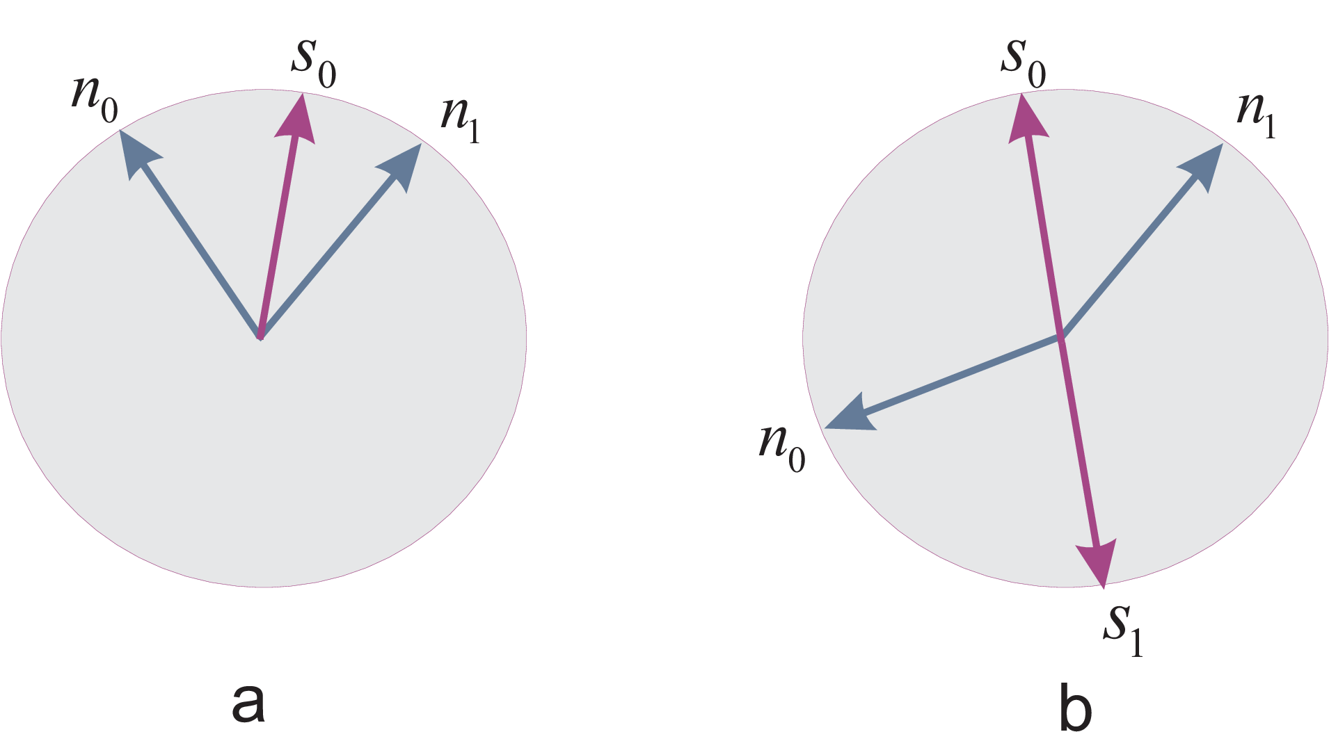
In the following discussion and proofs, we designate the corresponding CC states in the above two cases by $\sigma_{cc}^{+}$ (case ${\bf i}$) and $\sigma_{cc}^{-}$ (case ${\bf ii}$) respectively.

Note that in case i), the classically correlated state is indeed a product state while in the other case, it has some classical correlations. In both cases, the fidelity between the state $\rho$ and this nearest state $\sigma_{cc}$ is given by

$$F_{max}=F(\rho,\sigma_{cc})=\frac{1}{2}\left[\sqrt{p_{0}(1+\xi)(1+{\bf n}_{0}\cdot{\bf s}_{0})}+\sqrt{p_{1}(1-\xi)(1+{\bf n}_{1}\cdot{\bf s}_{1})}\right].$$

(52)

In particular it directly follows that when $p_{0}=p_{1}=\frac{1}{2}$, the fidelity is given by $F_{max}=\sqrt{\frac{1}{2}\left[1+\sqrt{{\frac{1+|{n}_{0}\cdot{n}_{1}|}{2}}}\right]}$, implying that the largest quantum correlations belongs to states of the form

$$\rho=\frac{1}{2}\left[|0\rangle\langle 0|\otimes|0\rangle\langle 0|+|\phi\rangle\langle\phi|\otimes|1\rangle\langle 1|\right],$$

(53)

where $|\phi\rangle=\frac{1}{\sqrt{2}}(|0\rangle+e^{i\phi}|1\rangle)$ is an equatorial states on the Bloch sphere.

Lemma 1: The nearest classically correlated state ${\sigma_{cc}}$ is of the form

$$\sigma_{cc}={\bf x}_{0}\otimes|0\rangle\langle 0|+{\bf x}_{1}\otimes|1\rangle\langle 1|.$$

(54)

Note that by this lemma, we are excluding the possibility of the second bases to be any bases other than $|0\rangle\langle 0|$ and $|1\rangle\langle 1|$.

Proof: We first rewrite $\rho$ in the matrix notation as

$$\rho=\left(\begin{array}[]{cc}p_{0}\rho_{0}&0\\ 0&p_{1}\rho_{1}\end{array}\right),$$

(55)

where $\rho_{0}=|{\bf n}_{0}\rangle\langle{\bf n}_{0}|$ and $\rho_{1}=|{\bf n}_{1}\rangle\langle{\bf n}_{1}|$. This state clearly has the invariance property

$$(I\otimes Z)\rho(I\otimes Z)=\rho,$$

(56)

where $Z=\left(\begin{array}[]{cc}1&0\\ 0&-1\end{array}\right)$. Now assume that $\sigma_{cc}$ be a state which has the maximum fidelity with this state. Then from the above invariance and from the invariance property of the fidelity, under local unitary transformations, we find

$$F(\rho,{\sigma_{cc}})=F((I\otimes Z)\rho(I\otimes Z),{\sigma_{cc}})=F(\rho,(I\otimes Z){\sigma_{cc}}(I\otimes Z))$$

(57)

Therefore either ${\sigma_{cc}}$ and $(I\otimes Z){\sigma_{cc}}(I\otimes Z)$ are the same state, or else we can form an invariant state in the form

$$\sigma^{new}_{cc}=\frac{1}{2}({\sigma_{cc}}+(I\otimes Z){\sigma_{cc}}(I\otimes Z))$$

(58)

which has higher fidelity with $\rho$ in view of the convex property of the fidelity $F(\rho,\lambda\sigma_{1}+(1-\lambda)\sigma_{2})\geq\lambda F(\rho,\sigma_{1})+(1-\lambda)F(\rho,\lambda\sigma_{2})$. Note that since we have to make this maximization over the set of classically correlated states, it is important to note if ${\sigma_{cc}}$ is classically correlated, then ${\sigma_{cc}}^{new}$ is also classically correlated. This shows that the closest CC state to $\rho$ has the same invariance property (56) and so is of the same form as $\rho$ itself, hence the lemma is proved.

Lemma 2: The classically correlated state ${\sigma_{cc}}$ nearest to (48) is of the form

$${\sigma_{cc}}=q_{0}|{\bf s}_{0}\rangle\langle{\bf s}_{0}|\otimes|0\rangle\langle 0|+q_{1}|{\bf s}_{1}\rangle\langle{\bf s}_{1}|\otimes|1\rangle\langle 1|,$$

(59)

where ${\bf s}_{0}$ and ${\bf s}_{1}$ are two unit vectors on the Bloch sphere which are co-linear, (i.e. they are either the same ${\bf s}_{1}={\bf s}_{0}$ or opposite to each other ${\bf s}_{1}=-{\bf s}_{0}$). By this lemma we are excluding the possibility of ${\bf x}_{0}$ and ${\bf x}_{1}$ to be mixed states.

Proof: The proof of this lemma is actually is by calculation. From lemma 1, and noting that $[{\bf x}_{0},{\bf x}_{1}]=0$, we let $\{|{\bf s}\rangle,|-{\bf s}\rangle\}$ be the basis which diagonalize ${\bf x}_{0}$ and ${\bf x}_{1}$. Then the state $\sigma_{cc}$ will be of the form

$${\sigma_{cc}}=\left(q_{00}|{\bf s}\rangle\langle{\bf s}|+q_{10}|-{\bf s}\rangle\langle-{\bf s}|\right)\otimes|0\rangle\langle 0|+\left(q_{01}|{\bf s}\rangle\langle{\bf s}|+q_{11}|-{\bf s}\rangle\langle-{\bf s}|\right)\otimes|1\rangle\langle 1|.$$

(60)

We want to maximize the fidelity of the state (48) with this state, given the general definition $F(\rho,\sigma)=tr\sqrt{\rho^{\frac{1}{2}}\sigma\rho^{\frac{1}{2}}}$. From the form of (48) and (60) and the purity of all the states $|{\bf n}_{i}\rangle$ and $|{\bf s}_{i}\rangle$, and using the fact that $|\langle{\bf m}|{\bf n}\rangle|=\sqrt{\frac{1+{\bf m}\cdot{\bf n}}{2}}$, we find

$$F(\rho,\sigma_{cc})=\sqrt{\frac{p_{0}}{2}(q_{00}+q_{10}+(q_{00}-q_{10}){\bf s}\cdot{\bf n}_{0})}+\sqrt{\frac{p_{1}}{2}(q_{01}+q_{11}+(q_{01}-q_{11}){\bf s}\cdot{\bf n}_{1})}.$$

(61)

We now have to maximize this expression with respect to the variables $q_{ij}$, subject to the constraint $\sum_{ij}q_{ij}=1$ and the direction of the vector ${\bf s}$. The first thing to note is that setting the variations of $F$ with respect to ${\bf s}$ (using Lagrange multipliers to account for its normalization), one finds that ${\bf s}$ should lie in the same plane as ${\bf n}_{0}$ and ${\bf n}_{1}$. One then set the variations of $F$ with respect to $q_{ij}$ equal to zero, again taking into account the constraint ($\sum_{ij}q_{ij}=1$) with a Lagrange multiplier. The result is that from all the $q_{ij}$ only two should be non-vanishing. This proves the lemma.

Having this, and taking for concreteness $q_{11}=q_{10}=0$ we now re-write (61) as

$$F(\rho,\sigma)=\sqrt{\frac{p_{0}q_{0}(1+{\bf n}_{0}\cdot{\bf s}_{0})}{2}}+\sqrt{\frac{p_{1}q_{1}(1+{\bf n}_{1}\cdot{\bf s}_{1})}{2}}$$

(62)

Where we now take either ${\bf s}_{1}={\bf s}_{0}$ or ${\bf s}_{1}=-{\bf s}_{0}$ in order not to loose generality. To proceed with the optimization, we now paramaterize the vectors ${\bf n}_{0}$ and ${\bf n}_{1}$ and ${\bf s}_{0}$ as in figure (6), that is:

$${\bf n}_{0}=(-\sin\alpha,\cos\alpha),\hskip 28.45274pt{\bf n}_{1}=(\sin\alpha,\cos\alpha),\hskip 28.45274pt{\bf s}_{0}=(\sin\theta,\cos\theta),\hskip 28.45274pt{\bf s}_{1}=\pm{\bf s}_{0}.$$

(63)

Also we set

$$q_{0}:=\frac{1+\xi}{2},\hskip 28.45274ptq_{1}:=\frac{1-\xi}{2},$$

(64)

where $\-1\leq\xi\leq 1$. Using (63) and (64), equation (62) is rewritten as

$$F(\rho,{\sigma_{cc}}^{+})=\sqrt{\frac{p_{0}(1+\xi)}{2}}\cos(\frac{\theta+\alpha}{2})+\sqrt{\frac{p_{1}(1-\xi)}{2}}\cos(\frac{\theta-\alpha}{2}).$$

(65)

and

$$F(\rho,{\sigma_{cc}}^{-})=\sqrt{\frac{p_{0}(1+\xi)}{2}}\cos(\frac{\theta+\alpha}{2})+\sqrt{\frac{p_{1}(1-\xi)}{2}}\sin(\frac{\theta-\alpha}{2}).$$

(66)

We now have to maximize each of these expressions with respect to the two parameters $\theta$ and $\xi$. It is convenient to do this for the two states $\sigma_{cc}^{\pm}$ separately.

Case i: Consider the expression (65). Setting $\frac{\partial F}{\partial\xi}=0$, we find

$$\sqrt{\frac{p_{0}}{1+\xi}}\cos(\frac{\theta+\alpha}{2})=\sqrt{\frac{p_{1}}{1-\xi}}\cos(\frac{\theta-\alpha}{2}).$$

(67)

Setting $\frac{\partial F}{\partial\theta}=0$, we obtain

$$\sqrt{p_{0}(1+\xi)}\sin(\frac{\theta+\alpha}{2})=-\sqrt{p_{1}(1-\xi)}\sin(\frac{\theta-\alpha}{2}).$$

(68)

From these two expressions, one can obtain the optimal values of $\xi$ and $\theta$, which ultimately determine the vector ${\bf s}_{0}$ and $q_{0}$ and hence the classically correlated state ${\sigma^{+}}_{cc}$ which has the maximal fidelity with the given state $\rho.$ To proceed further, we note that by multiplying equations (67) and (68) we obtain

$$p_{0}\sin(\theta+\alpha)=p_{1}\sin(\alpha-\theta).$$

(69)

This equation determines the angle $\theta$. Dividing (68) by (67) we obtain

$$(1+\xi)\tan(\frac{\alpha+\theta}{2})=(1-\xi)\tan(\frac{\alpha-\theta}{2}).$$

(70)

From this second equation we can then determine $\xi$. In order to express everything in terms of the original data of the problem, that is $p_{0}$, ${\bf n}_{0}$ and ${\bf n}_{1}$, we note equation (69) is equivalent to

$$p_{0}{\bf n}_{0}\times{\bf s}_{0}=p_{1}{\bf n}_{1}\times{\bf s}_{0},$$

(71)

from which we find that ${\bf s}\propto p_{0}{\bf n}_{0}+p_{1}{\bf n}_{1}$ or after normalization,

$${\bf s}_{0}=\frac{p_{0}{\bf n}_{0}+p_{1}{\bf n}_{1}}{\sqrt{1-2p_{0}p_{1}(1-{\bf n}_{0}\cdot{\bf n}_{1}})}.$$

(72)

To express $\xi$ directly in terms of the initial data of the problem we note that after some algebra, equation (70) gives

$$\xi=-\frac{\sin\theta}{\sin\alpha}.$$

(73)

It is now straightforward to start from (73) and verify the following relations:

$$\sin\alpha=\sqrt{\frac{1-{\bf n}_{0}\cdot{\bf n}_{1}}{2}},\hskip 28.45274pt{\bf x}=\frac{{\bf n}_{1}-{\bf n}_{0}}{\sqrt{2(1-{\bf n}_{0}\cdot{\bf n}_{1})}}.$$

(74)

From the fact that $\sin\theta={\bf x}\cdot{\bf s}_{0}$ and the above expressions, we can put everything together using (72) and (74) and obtain $\xi$ as

$$\xi=\frac{p_{0}-p_{1}}{\sqrt{1-2p_{0}p_{1}(1-{\bf n}_{0}\cdot{\bf n}_{1})}}.$$

(75)

In this way we obtain the one of the nearest classically correlated state to our quantum-classical state $\rho$.

References

- [1] Alexander Streltsov, Hermann Kampermann, and Dagmar Bruß, Phys. Rev. Lett. 107, 170502 (2011).
- [2] M. A. Nielsen, and I. L. Chuang;Quantum computation and quantum information,Cambridge University Press, Cambridge, 2000.
- [3] C.Macchiavello, G.M.Palma and A. Zeilinger, Quantum computation and quantum information theory, World Scientific, Singapore, 2001.
- [4] A. Datta, A. Shaji, and C. M. Caves, Phys. Rev. Lett. 100, 050502 (2008).
- [5] E. Knill and R. Laflamme, Phys. Rev. Lett. 81, 5672 (1998).
- [6] M. Piani, P. Horodecki, R. Horodecki, Phys. Rev. Lett. 100, 090502 (2008).
- [7] D. Cavalcanti, L. Aolita, S. Boixo, K. Modi, M. Piani, A. Winter, Phys. Rev. A 83, 032324 (2011); V. Madhok, A. Datta, Phys. Rev. A 83, 032323 (2011).
- [8] B. Dakic, Y. O. Lipp, X. Ma, M. Ringbauer, S. Kropatschek,S. Barz, T. Paterek, V. Vedral, A. Zeilinger, C. Brukner and Ph. Walther, Nature Physics 8, 666670 (2012)
- [9] A. Streltsov, H. Kampermann, and D. Bruß, Phys. Rev. Lett. 108, 250501 (2012).
- [10] T. K. Chuan, J. Maillard, K. Modi, T. Paterek, M. Paternostro, and M. Piani, arXiv:1203.1268v2 (2012);
- [11] L. Roa, J. C. Retamal, and M. Alid-Vaccarezza, Phys. Rev. Lett. 107, 080401 (2011)
- [12] H. Ollivier and W. H. Zurek, Phys. Rev. Lett. 88, 017901 (2001); L. Henderson and V. Vedral, J. Phys. A: Math. Gen. 34, 6899 (2001).
- [13] J. Oppenheim, M. Horodecki, P. Horodecki and R. Horodecki, Phys. Rev. Lett. 89, 180402 (2002); M. Horodecki, P. Horodecki, R. Horodecki, J. Oppenheim, A. Sen, U. Sen, and B. Synak-Radtke, Phys. Rev. A 71, 062307 (2005).
- [14] K. Modi, T. Paterek, W. Son, V. Vedral, and M. Williamson, Phys. Rev. Lett. 104, 080501 (2010).
- [15] B. Dakic, V. Vedral, and C. Brukner, Phys. Rev. Lett. 105, 190502 (2010).
- [16] G. Adesso and A. Datta, Phys. Rev. Lett. 105, 030501 (2010); P. Giorda and M. G. A. Paris, Phys. Rev. Lett. 105, 020503 (2010).
- [17] M. Gessner, E-M. Laine, H. Peter Breuer, J. Piilo, Phys. Rev. A 85, 052122 (2012).
- [18] W. H. Zurek, Phys. Rev. A 67, 012320 (2003).
- [19] A. Streltsov, H. Kampermann, and D. Bruß, Phys. Rev. Lett. 106, 160401 (2011); M. Piani, S. Gharibian, G. Adesso, J. Calsamiglia, P. Horodecki, and A. Winter, Phys. Rev. Lett. 106, 220403 (2011); P. Perinotti, Phys. Rev. Lett. 108, 120502 (2012).
- [20] Takafumi Nakano, Marco Piani, Gerardo Adesso, arXiv:1211.4022.
- [21] F. Ciccarello, V. Giovannetti, Phys. Rev. A 85, 010102(R) (2012); F. Ciccarello, V. Giovannetti, Phys. Rev. A 85, 022108 (2012)
- [22] X. Hu, H. Fan, D. L. Zhou, W. Liu, Phys. Rev. A 85, 032102 (2012).
- [23] X. Hu, H. Fan, D. L. Zhou and W. Liu, arXiv:1203.6149 (2012).
- [24] F. Galve, F. Plastina, M. G. A. Paris, R. Zambrini; arXiv:1208.5605.
- [25] A. Shabani and D. A. Lidar, Phys. Rev. Lett. 102, 100402 (2009); L. Mazzola, J. Piilo, and S. Maniscalco, Phys. Rev. Lett. 104, 200401 (2010); B. Bellomo, R. Lo Franco, and G. Compagno Phys. Rev. A. 86, 012312 (2012); R. Lo Franco, B. Bellomo, E. Andersson, and G. Compagno, Phys. Rev. A. 85, 032318 (2012)
- [26] X. Hu, Y. Gu, Q. Gong, G.Guo, Phys. Rev. A 84, 022113 (2011).
- [27] B. Groisman, D. Kenigsberg and T. Mor, arXiv:quant-ph/0703103.
- [28] C. King, M. B. Ruskai. IEEE Trans. Info. Theory, 47, 192-209 (2001); M Beth Ruskai, S Szarek, E Werner. Linear algebra and its applications, 2002, Elsevier.