Convex Hull of Two Orthogonal Disks

Steven R. Finch

March 12, 2016

Abstract

Three configurations of two perpendicular disks in $\mathbb{R}^{3}$ are examined, the first in which the disks share centers and the other two in which the disks touch at precisely one point. Volume, surface area and mean width calculations dominate the discussion. Integrated mean curvature also appears as an indirect way to compute mean width.

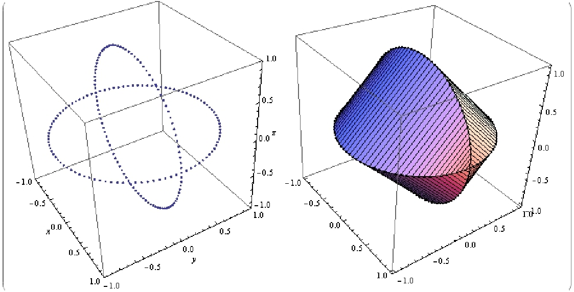
Our investigation begins with a theoretical question about experimental data. Example 1 is the convex hull of the following two orthogonal disks in $\mathbb{R}^{3}$ :

\begin{array}[c]{ccccc}\left\{(x,y,z):x^{2}+y^{2}\leq 1\text{ \&\ }z=0\right\}&&\text{and}&&\left\{(x,y,z):x^{2}+z^{2}\leq 1\text{ \&\ }y=0\right\}.\end{array}

We can numerically evaluate the volume $VL$ , surface area $AR$ and mean width $MW$ of the corresponding solid domain in Figure 1 using [1]:

\begin{array}[c]{ccccc}VL_{1}\approx 2.666,&&AR_{1}\approx 10.28,&&MW_{1}\approx 1.869.\end{array}

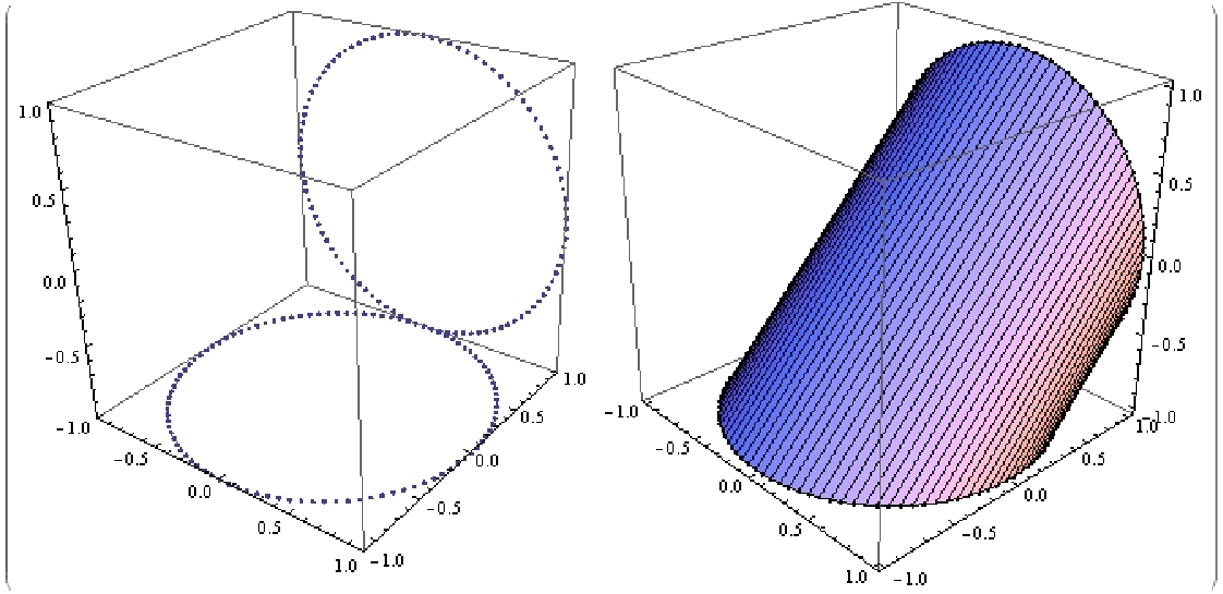
Example 2 is the convex hull of the two disks:

\begin{array}[c]{ccccc}\left\{(x,y,z):x^{2}+y^{2}\leq 1\text{ \&\ }z=-1\right\}&&\text{and}&&\left\{(x,y,z):x^{2}+z^{2}\leq 1\text{ \&\ }y=1\right\}\end{array}

with corresponding solid domain in Figure 2 and

\begin{array}[c]{ccccc}VL_{2}\approx 3.141,&&AR_{2}\approx 13.92,&&MW_{2}\approx 2.277.\end{array}

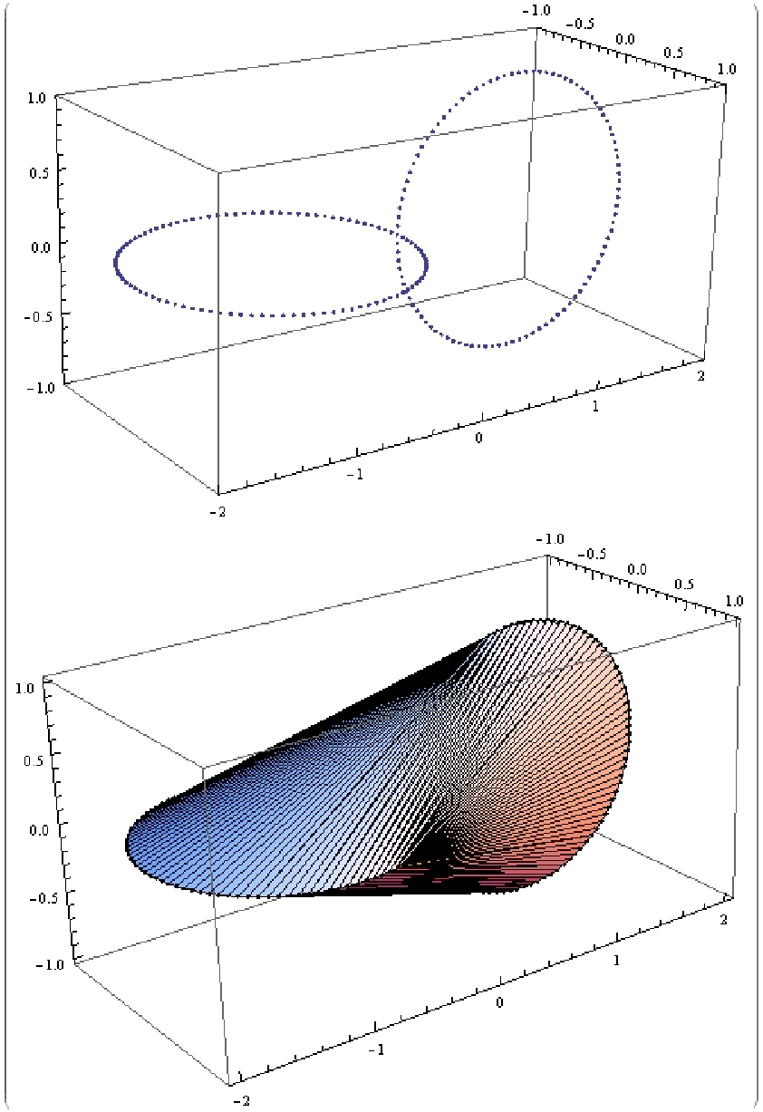
Example 3 is the convex hull of the two disks:

\begin{array}[c]{ccccc}\left\{(x,y,z):x^{2}+(y+1)^{2}\leq 1\text{ \&\ }z=0\right\}&&\text{and}&&\left\{(x,y,z):(y-1)^{2}+z^{2}\leq 1\text{ \&\ }x=0\right\}\end{array}

with corresponding solid domain in Figure 3 and

\begin{array}[c]{ccccc}VL_{3}\approx 3.627,&&AR_{3}\approx 15.97,&&MW_{3}\approx 2.645.\end{array}

Of the nine constants, just two ( $VL_{1}=8/3$ and $VL_{2}=\pi$ ) are readily identifiable. What are exact closed-form expressions for the remaining constants?

Given $\Omega$ to be a convex body in $\mathbb{R}^{3}$ , a width is the distance between a pair of parallel $\Omega$ -supporting planes. Every unit vector $v\in\mathbb{R}^{3}$ determines a unique such pair of planes orthogonal to $v$ and hence a width $w(v)$ . Let $v$ be uniformly distributed on the unit sphere $S^{2}\subset$ $\mathbb{R}^{3}$ . Then $w$ is a random variable and its average value is the mean width of $\Omega$ . Three numerical characteristics of $\Omega$ – volume, surface area and mean width – are central to our study. These quantities, along with the Euler characteristic, form a basis of the space of all additive continuous measures that are invariant under rigid motions in $\mathbb{R}^{3}$ .

“The mean width is a new measure on three-dimensional solids that enjoys equal rights with volume and surface area” [2], hence much of this paper is devoted to computing $MW$ for our three examples. What we call the direct approach is based on the definition of $MW$ ; what we call the indirect approach utilizes a connection between $MW$ and integrated mean curvature (often called ”integral” or “total” mean curvature). This connection is suggested in the materials science [3, 4] and astrophysics literature [5, 6]; the closest claim to a proof appears in [7], based chiefly on [8]. Our paper therefore also serves to confirm the validity of the indirect approach for certain non-polyhedral test cases.¹¹ 1 On page 513 of [7], mean curvature $\mathcal{K}$ is defined as the average of the two principal curvatures, but this is inconsistent with [8], which takes $\mathcal{K}$ to be the sum. We follow [8], defining $2H=\mathcal{K}$ . Our formula correctly gives $MW=(\ell+\pi r)/2$ for a right circular cylinder of length $\ell$ , radius $r$ [9, 10].

1 Example 1

The boundary $\partial\Omega$ of the convex hull $\Omega$ here is trivially given by the surface

z=\pm\left(\sqrt{1-x^{2}}-\left|y\right|\right)

over the planar region $x^{2}+y^{2}\leq 1$ . Let

\begin{array}[c]{ccc}\varphi(x,y)=\sqrt{1-x^{2}}-y,&&x^{2}+y^{2}\leq 1\text{ \&\ }y\geq 0\end{array}

then $\varphi_{x}$ , $\varphi_{y}$ , $\varphi_{xx}$ , $\varphi_{xy}$ , $\varphi_{yy}$ denote first/second-order partial derivatives of $\varphi$ and

VL_{1}=4{\displaystyle\int\limits_{-1}^{1}}{\displaystyle\int\limits_{0}^{\sqrt{1-x^{2}}}}\varphi(x,y)\,dy\,dx=\frac{8}{3},

	$\displaystyle AR_{1}$	$\displaystyle={\displaystyle\int\limits_{\partial\Omega}}dS=4{\displaystyle\int\limits_{-1}^{1}}{\displaystyle\int\limits_{0}^{\sqrt{1-x^{2}}}}\sqrt{1+\varphi_{x}^{2}+\varphi_{y}^{2}}\,dy\,dx=2(2+\pi)$
		$\displaystyle=10.2831853071795864769252867....$

1.1 Indirect Approach

Let $\partial\Omega^{+}$ denote the upper portion of $\partial\Omega$ and $\partial\Omega^{-}$ denote the lower portion. On the one hand, the mean curvature of $\partial\Omega^{+}$ is

H(x,y)=-\frac{\left(1+\varphi_{x}^{2}\right)\varphi_{yy}-2\varphi_{x}\varphi_{y}\varphi_{xy}+\left(1+\varphi_{y}^{2}\right)\varphi_{xx}}{2\left(1+\varphi_{x}^{2}+\varphi_{y}^{2}\right)^{3/2}}=\frac{1}{\left(2-x^{2}\right)^{3/2}}

over the open region $x^{2}+y^{2}<1$ & $y>0$ . It follows that

H\,dS=H(x,y)\sqrt{1+\varphi_{x}^{2}+\varphi_{y}^{2}}\,dy\,dx=\frac{1}{\left(2-x^{2}\right)^{3/2}}\sqrt{\frac{2-x^{2}}{1-x^{2}}}\,dy\,dx=\frac{dy\,dx}{\left(2-x^{2}\right)\sqrt{1-x^{2}}}.

On the other hand, the exterior dihedral angle on the semicircular edge $x^{2}+y^{2}=1$ & $y\geq 0$ is

\alpha=2\arccos\left(\frac{1}{\sqrt{2-x^{2}}}\right)

because the unit exterior normal vector to $\partial\Omega^{+}$ is

\frac{1}{\sqrt{1+\varphi_{x}^{2}+\varphi_{y}^{2}}}\left(-\varphi_{x},-\varphi_{y},1\right)=\sqrt{\frac{1-x^{2}}{2-x^{2}}}\left(\frac{x}{\sqrt{1-x^{2}}},1,1\right)=\frac{1}{\sqrt{2-x^{2}}}\left(x,y,y\right)

and the unit exterior normal vector to the cylinder $x^{2}+y^{2}=1$ is $(x,y,0)$ . The dot product of the two vectors is $1/\sqrt{2-x^{2}}$ ; we multiply the angle by two since the dihedral angle between $\partial\Omega^{+}$ and $\partial\Omega^{-}$ is twice the preceding angle. In terms of arclength $s=\theta$ , $0\leq\theta\leq\pi$ , we have

\alpha\,ds=2\arccos\left(\frac{1}{\sqrt{2-\cos^{2}\theta}}\right)d\theta.

The surface $\partial\Omega$ is piecewise continuously differentiable and has $n=4$ smooth edges $\varepsilon_{j}$ with (non-constant) dihedral angles $\alpha_{j}$ , $1\leq j\leq n$ . From the general formula

MW=\frac{1}{2\pi}{\displaystyle\int\limits_{\partial\Omega}}H\,dS+\frac{1}{4\pi}\sum_{j=1}^{n}{\displaystyle\int\limits_{\varepsilon_{j}}}\alpha_{j}\,ds,

we deduce that

	$\displaystyle MW_{1}$	$\displaystyle=\frac{4}{2\pi}{\displaystyle\int\limits_{-1}^{1}}{\displaystyle\int\limits_{0}^{\sqrt{1-x^{2}}}}\frac{dy\,dx}{\left(2-x^{2}\right)\sqrt{1-x^{2}}}+\frac{8}{4\pi}{\displaystyle\int\limits_{0}^{\pi}}\arccos\left(\frac{1}{\sqrt{2-\cos^{2}\theta}}\right)d\theta$
		$\displaystyle=-\frac{1}{\pi}\left(2\sqrt{2}\ln\left(-1+\sqrt{2}\right)-4\operatorname{Li}\nolimits_{2}\left(-1+\sqrt{2}\right)+4\operatorname{Li}\nolimits_{2}\left(1-\sqrt{2}\right)\right)$
		$\displaystyle=1.8697727582861870379136441...$

where $\operatorname*{Li}\nolimits_{2}$ is the dilogarithm

\begin{array}[c]{ccc}\operatorname*{Li}\nolimits_{2}(x)={\displaystyle\sum\limits_{k=1}^{\infty}}\dfrac{x^{k}}{k^{2}}=-{\displaystyle\int\limits_{0}^{x}}\dfrac{\ln(1-t)}{t}dt,&&|x|\leq 1.\end{array}

1.2 Direct Approach

Consider the portion of $\partial\Omega$ in the first octant only. In this octant, an $\Omega$ -supporting plane $P^{d}:$

\begin{array}[c]{ccc}\dfrac{a}{d}x+\dfrac{b}{d}y+\dfrac{c}{d}z=1&&\text{(with coefficients }a>0,b>0,c>0\text{ and scaling factor }d>0\text{)}\end{array}

has an associated line $\ L_{xy}^{d}:$

\dfrac{a}{d}x+\dfrac{b}{d}y=1\text{ \&\ }z=0

in the $xy$ -plane and an associated line $L_{xz}^{d}:$

\dfrac{a}{d}x+\dfrac{c}{d}z=1\text{ \&\ }y=0

in the $xz$ -plane. Assume WLOG that $a^{2}+b^{2}+c^{2}=1$ . The distance of $P^{d}$ from the origin $O$ is $d$ . Also,

\begin{array}[c]{ccccc}\text{distance of }L_{xy}^{d}\text{ from }O\text{ is }\dfrac{d}{\sqrt{a^{2}+b^{2}}}&&\text{and}&&\text{distance of }L_{xz}^{d}\text{ from }O\text{ is }\dfrac{d}{\sqrt{a^{2}+c^{2}}}.\end{array}

The largest $d$ such that

\begin{array}[c]{ccccc}L_{xy}^{d}\text{ supports }x^{2}+y^{2}=1&&\text{or}&&L_{xz}^{d}\text{ supports }x^{2}+z^{2}=1\end{array}

is thus

d=\max\left\{\sqrt{a^{2}+b^{2}},\sqrt{a^{2}+c^{2}}\right\}.

Let

\begin{array}[c]{ccccc}a=\cos\theta\sin\phi,&&b=\sin\theta\sin\phi,&&c=\cos\phi\end{array}

where $0\leq\theta\leq\pi/2$ , $0\leq\phi\leq\pi/2$ . To ensure uniformity, think of $(\theta,\phi)$ as possessing joint density $\frac{2}{\pi}\sin\phi$ . We have

	$\displaystyle MW_{1}$	$\displaystyle=2{\displaystyle\int\limits_{0}^{\pi/2}}\,{\displaystyle\int\limits_{0}^{\pi/2}}\max\left\{\sin\phi,\sqrt{\cos^{2}\theta\sin^{2}\phi+\cos^{2}\phi}\right\}\frac{2}{\pi}\sin\phi\,d\phi\,d\theta$
		$\displaystyle=\frac{8}{\pi}{\displaystyle\int\limits_{0}^{\pi/2}}\,{\displaystyle\int\limits_{\xi(\theta)}^{\pi/2}}\sin^{2}\phi\,d\phi\,d\theta=1.8697727582861870379136441...$

where

\xi(\theta)=\arccos\left(\frac{\sin\theta}{\sqrt{2-\cos^{2}\theta}}\right)

is the required solution (for $\phi$ in terms of $\theta$ ) of the equation

\sin\phi=\sqrt{\cos^{2}\theta\sin^{2}\phi+\cos^{2}\phi}.

2 Example 2

The curved portions of the boundary $\partial\Omega$ of the convex hull $\Omega$ here are given by $z=\varphi(x,y)$ and $z=\psi(x,y)$ , where

\begin{array}[c]{ccc}\varphi(x,y)=\sqrt{1-x^{2}}+y-1,&&|x|\leq 1,\text{ }|y|\leq 1\text{ \&\ }y\geq-\sqrt{1-x^{2}},\end{array}

\begin{array}[c]{ccc}\psi(x,y)=-\sqrt{1-x^{2}}+y-1,&&|x|\leq 1,\text{ }|y|\leq 1\text{ \&\ }y\geq\sqrt{1-x^{2}}.\end{array}

The flat portions of $\partial\Omega$ are the two disks, one of which is given by $z=-1$ over $x^{2}+y^{2}\leq 1$ . These facts contribute to the following:

VL_{2}={\displaystyle\int\limits_{-1}^{1}}{\displaystyle\int\limits_{-\sqrt{1-x^{2}}}^{\sqrt{1-x^{2}}}}\left(\varphi(x,y)+1\right)\,dy\,dx+{\displaystyle\int\limits_{-1}^{1}}{\displaystyle\int\limits_{\sqrt{1-x^{2}}}^{1}}\left(\varphi(x,y)-\psi(x,y)\right)\,dy\,dx=\pi,

	$\displaystyle AR_{2}$	$\displaystyle=2\pi+{\displaystyle\int\limits_{-1}^{1}}{\displaystyle\int\limits_{-\sqrt{1-x^{2}}}^{1}}\sqrt{1+\varphi_{x}^{2}+\varphi_{y}^{2}}\,dy\,dx+{\displaystyle\int\limits_{-1}^{1}}{\displaystyle\int\limits_{\sqrt{1-x^{2}}}^{1}}\sqrt{1+\psi_{x}^{2}+\psi_{y}^{2}}\,dy\,dx$
		$\displaystyle=2\left(\pi+2\sqrt{2}E\left(\tfrac{1}{2}\right)\right)$
		$\displaystyle=13.9235808852350105127348109...$

where

E(\mu)={\displaystyle\int\limits_{0}^{\pi/2}}\sqrt{1-\mu\sin(\theta)^{2}}\,d\theta={\displaystyle\int\limits_{0}^{1}}\sqrt{\dfrac{1-\mu\,t^{2}}{1-t^{2}}}\,dt

is the complete elliptic integral of the second kind.

2.1 Indirect Approach

Let $\partial\Omega^{+}$ denote the curved portion of $\partial\Omega$ prescribed by $\varphi$ and $\partial\Omega^{-}$ denote the curved portion prescribed by $\psi$ . We have

	$\displaystyle-\frac{\left(1+\varphi_{x}^{2}\right)\varphi_{yy}-2\varphi_{x}\varphi_{y}\varphi_{xy}+\left(1+\varphi_{y}^{2}\right)\varphi_{xx}}{2\left(1+\varphi_{x}^{2}+\varphi_{y}^{2}\right)^{3/2}}$	$\displaystyle=\frac{1}{\left(2-x^{2}\right)^{3/2}}$
		$\displaystyle=-\frac{\left(1+\psi_{x}^{2}\right)\psi_{yy}-2\psi_{x}\psi_{y}\psi_{xy}+\left(1+\psi_{y}^{2}\right)\psi_{xx}}{2\left(1+\psi_{x}^{2}+\psi_{y}^{2}\right)^{3/2}}$

everywhere and hence

H\,dS=\frac{dy\,dx}{\left(2-x^{2}\right)\sqrt{1-x^{2}}}

as previously. It follows that

{\displaystyle\int\limits_{\partial\Omega}}H\,dS={\displaystyle\int\limits_{-1}^{1}}{\displaystyle\int\limits_{-\sqrt{1-x^{2}}}^{1}}\frac{dy\,dx}{\left(2-x^{2}\right)\sqrt{1-x^{2}}}+{\displaystyle\int\limits_{-1}^{1}}{\displaystyle\int\limits_{\sqrt{1-x^{2}}}^{1}}\frac{dy\,dx}{\left(2-x^{2}\right)\sqrt{1-x^{2}}}=\sqrt{2}\pi.

Let $\varepsilon$ denote the circular edge $x^{2}+y^{2}=1$ & $z=-1$ . Clearly $\partial\Omega^{+}\cap\varepsilon$ is the semicircle with $y=-\sqrt{1-x^{2}}$ whereas $\partial\Omega^{-}\cap\varepsilon$ is the semicircle with $y=\sqrt{1-x^{2}}$ . The exterior dihedral angle on $\varepsilon$ is

\alpha=\arccos\left(\frac{y}{\sqrt{2-x^{2}}}\right)

because the unit exterior normal vector to $\partial\Omega^{+}$ , $\partial\Omega^{-}$ is

\frac{1}{\sqrt{1+\varphi_{x}^{2}+\varphi_{y}^{2}}}\left(-\varphi_{x},-\varphi_{y},1\right)=\sqrt{\frac{1-x^{2}}{2-x^{2}}}\left(\frac{x}{\sqrt{1-x^{2}}},-1,1\right)=\frac{1}{\sqrt{2-x^{2}}}\left(x,y,-y\right),

\frac{1}{\sqrt{1+\psi_{x}^{2}+\psi_{y}^{2}}}\left(\psi_{x},\psi_{y},-1\right)=\sqrt{\frac{1-x^{2}}{2-x^{2}}}\left(\frac{x}{\sqrt{1-x^{2}}},1,-1\right)=\frac{1}{\sqrt{2-x^{2}}}\left(x,y,-y\right)

respectively and the unit exterior normal vector to the horizontal disk is $(0,0,-1)$ . The dot product of the two vectors is $y/\sqrt{2-x^{2}}$ . An identical argument applies for the circular edge $x^{2}+z^{2}=1$ & $y=1$ . In terms of arclength $s=\theta$ , $0\leq\theta\leq 2\pi$ , we obtain

2{\displaystyle\int\limits_{\varepsilon}}\alpha\,ds=2{\displaystyle\int\limits_{0}^{2\pi}}\arccos\left(\frac{\sin\theta}{\sqrt{2-\cos^{2}\theta}}\right)d\theta=2\pi^{2}

which leads to the conclusion that

MW_{2}=\frac{1}{2\pi}\left(\sqrt{2}\pi\right)+\frac{1}{4\pi}\left(2\pi^{2}\right)=\frac{1}{2}\left(\sqrt{2}+\pi\right)=2.2779031079814441436321660....

2.2 Direct Approach

Consider the curved portion of $\partial\Omega$ in the halfspace $x\geq 0$ only. In this halfspace, an $\Omega$ -supporting plane $P^{d}:$

\begin{array}[c]{ccc}\dfrac{a}{d}x+\dfrac{b}{d}y+\dfrac{c}{d}z=1&&\text{(with coefficients }a>0,\,b,\,c\text{ and scaling factor }d>0\text{)}\end{array}

has associated lines $\ L_{xy}^{d}$ , $L_{xz}^{d}:$

\begin{array}[c]{ccc}\dfrac{a}{d}x+\dfrac{b}{d}y=\dfrac{d+c}{d}\text{ \&\ }z=-1,&&\dfrac{a}{d}x+\dfrac{c}{d}z=\dfrac{d-b}{d}\text{ \&\ }y=1.\end{array}

Assume WLOG that $a^{2}+b^{2}+c^{2}=1$ . The distance of $P^{d}$ from the origin $O$ is $d$ . Also,

\begin{array}[c]{ccccc}\text{distance of }L_{xy}^{d}\text{ from }O_{z}\text{ is }\dfrac{d+c}{\sqrt{a^{2}+b^{2}}}&&\text{and}&&\text{distance of }L_{xz}^{d}\text{ from }O_{y}\text{ is }\dfrac{d-b}{\sqrt{a^{2}+c^{2}}}\end{array}

where $O_{z}=(0,0,-1)$ and $O_{y}=(0,1,0)$ . The largest $d$ such that one of the unit circles is supported is thus

d=\max\left\{\sqrt{a^{2}+b^{2}}-c,\sqrt{a^{2}+c^{2}}+b\right\}.

We introduce spherical coordinates as before, but with $-\pi/2\leq\theta\leq\pi/2$ , $0\leq\phi\leq\pi$ instead. To ensure uniformity, think of $(\theta,\phi)$ as possessing joint density $\frac{1}{2\pi}\sin\phi$ . We have

	$\displaystyle MW_{2}$	$\displaystyle=2\,{\displaystyle\int\limits_{-\pi/2}^{\pi/2}}{\displaystyle\int\limits_{0}^{\pi}}\max\left\{\sin\phi-\cos\phi,\sqrt{\cos^{2}\theta\sin^{2}\phi+\cos^{2}\phi}+\sin\theta\sin\phi\right\}\frac{1}{2\pi}\sin\phi\,d\phi\,d\theta$
		$\displaystyle=\frac{2}{\pi}{\displaystyle\int\limits_{-\pi/2}^{\pi/2}}\,{\displaystyle\int\limits_{\xi(\theta)}^{\pi}}\left(\sin\phi-\cos\phi\right)\sin\phi\,d\phi\,d\theta=2.2779031079814441436321660...$

where

\xi(\theta)=\pi/2+\arctan\left(\sin\theta\right)

is the required solution (for $\phi$ in terms of $\theta$ ) of the equation

\sin\phi-\cos\phi=\sqrt{\cos^{2}\theta\sin^{2}\phi+\cos^{2}\phi}+\sin\theta\sin\phi.

3 Example 2 (Again)

Vinzant, using techniques in her thesis [11], computed that $\partial\Omega$ is given implicitly by the equation

	$\displaystyle 0$	$\displaystyle=-x^{2}+2y+x^{2}y-3y^{2}+y^{3}-2z-x^{2}z+6yz$
		$\displaystyle+x^{2}yz-5y^{2}z+y^{3}z-3z^{2}+5yz^{2}-2y^{2}z^{2}-z^{3}+yz^{3}$
		$\displaystyle=\left(y-1\right)\left(z+1\right)\left(x^{2}-2y+y^{2}+2z-2yz+z^{2}\right)$
		$\displaystyle=\left(y-1\right)\left(z+1\right)(z-\varphi(x,y))(z-\psi(x,y))$

verifying what we already know. She additionally gave an elegant parametric representation of the curved portion in $x\geq 0$ :

\begin{array}[c]{ccccccc}x=\sqrt{1-v^{2}},&&y=1-u+uv,&&z=-u-v+uv,&&0\leq u\leq 1\text{ \&\ }-1\leq v\leq 1\end{array}

which deserves further attention. In the following, we reproduce our results from the preceding section. The purpose in doing so is not to torture the reader, but rather to set the stage for Example 3 (for which a parametric representation is the only workable method available.) The Jacobian determinant²² 2 The fact that this has indefinite sign doesn’t affect the volume calculation.

\frac{\partial(x,y)}{\partial(u,v)}=\left|\begin{array}[c]{cc}x_{u}&x_{v}\\ y_{u}&y_{v}\end{array}\right|=\frac{(-1+v)v}{\sqrt{1-v^{2}}}

allows us to evaluate

VL_{2}=2{\displaystyle\int\limits_{0}^{1}}{\displaystyle\int\limits_{-1}^{1}}\left((-u-v+uv)+1\right)\frac{(-1+v)v}{\sqrt{1-v^{2}}}\,dv\,du=\pi.

Defining

\begin{array}[c]{ccc}E=\left(x_{u},y_{u},z_{u}\right)\cdot\left(x_{u},y_{u},z_{u}\right),&&G=\left(x_{v},y_{v},z_{v}\right)\cdot\left(x_{v},y_{v},z_{v}\right),\end{array}

F=\left(x_{u},y_{u},z_{u}\right)\cdot\left(x_{v},y_{v},z_{v}\right)

we have

	$\displaystyle AR_{2}$	$\displaystyle={\displaystyle\int\limits_{\partial\Omega}}dS=2\pi+2{\displaystyle\int\limits_{0}^{1}}{\displaystyle\int\limits_{-1}^{1}}\sqrt{EG-F^{2}}\,dv\,du$
		$\displaystyle=2\pi+2{\displaystyle\int\limits_{0}^{1}}{\displaystyle\int\limits_{-1}^{1}}\sqrt{\frac{(1-v)(1+v^{2})}{1+v}}\,dv\,du$
		$\displaystyle=2\left(\pi+2\sqrt{2}E\left(\tfrac{1}{2}\right)\right).$

Defining

\mathcal{N}=\frac{\left(x_{u},y_{u},z_{u}\right)\times\left(x_{v},y_{v},z_{v}\right)}{\left|\left(x_{u},y_{u},z_{u}\right)\times\left(x_{v},y_{v},z_{v}\right)\right|}=\left(\sqrt{\frac{1-v^{2}}{1+v^{2}}},\frac{v}{\sqrt{1+v^{2}}},-\frac{v}{\sqrt{1+v^{2}}}\right),

\begin{array}[c]{ccc}L=-\left(x_{u},y_{u},z_{u}\right)\cdot\mathcal{N}_{u},&&N=-\left(x_{v},y_{v},z_{v}\right)\cdot\mathcal{N}_{v},\end{array}

M=-\dfrac{1}{2}\left(\left(x_{u},y_{u},z_{u}\right)\cdot\mathcal{N}_{v}+\left(x_{v},y_{v},z_{v}\right)\cdot\mathcal{N}_{u}\right)

we have

	$\displaystyle{\displaystyle\int\limits_{\partial\Omega}}H\,dS$	$\displaystyle={\displaystyle\int\limits_{\partial\Omega}}\frac{EN-2FM+GL}{2\left(EG-F^{2}\right)}\,dS$
		$\displaystyle=2{\displaystyle\int\limits_{0}^{1}}{\displaystyle\int\limits_{-1}^{1}}\frac{EN-2FM+GL}{2\left(EG-F^{2}\right)}\sqrt{EG-F^{2}}\,dv\,du$
		$\displaystyle=2{\displaystyle\int\limits_{0}^{1}}{\displaystyle\int\limits_{-1}^{1}}\frac{1}{\left(1+v^{2}\right)^{3/2}}\sqrt{\frac{(1-v)(1+v^{2})}{1+v}}\,dv\,du$
		$\displaystyle=2{\displaystyle\int\limits_{0}^{1}}{\displaystyle\int\limits_{-1}^{1}}\frac{1}{1+v^{2}}\sqrt{\frac{1-v}{1+v}}\,dv\,du=\sqrt{2}\pi.$

The semicircular edge $x^{2}+z^{2}=1$ , $y=1$ & $x\geq 0$ corresponds to $u=0$ & $-1\leq v\leq 1$ . Call this $\varepsilon$ . The exterior dihedral angle is

\alpha=\arccos\left(\mathcal{N}\cdot(0,1,0)\right)=\arccos\left(\frac{v}{\sqrt{1+v^{2}}}\right)

and arclength $s$ satisfies

ds=\sqrt{x_{v}^{2}+z_{v}^{2}}\,dv=\frac{1}{\sqrt{1-v^{2}}}\,dv.

Consequently

4{\displaystyle\int\limits_{\varepsilon}}\alpha\,ds=4{\displaystyle\int\limits_{-1}^{1}}\frac{1}{\sqrt{1-v^{2}}}\arccos\left(\frac{v}{\sqrt{1+v^{2}}}\right)dv=2\pi^{2}

and

MW_{2}=\frac{1}{2\pi}\left(\sqrt{2}\pi\right)+\frac{1}{4\pi}\left(2\pi^{2}\right)=\frac{1}{2}\left(\sqrt{2}+\pi\right)

as was to be shown.

4 Example 3

Vinzant, using techniques in her thesis [11], computed that $\partial\Omega$ here is given implicitly by the equation

	$\displaystyle 0$	$\displaystyle=-4x^{4}+8x^{6}-16x^{2}y+36x^{4}y-16y^{2}+40x^{2}y^{2}+15x^{4}y^{2}+36x^{2}y^{3}+8y^{4}$
		$\displaystyle+6x^{2}y^{4}-y^{6}-8x^{2}z^{2}+24x^{4}z^{2}+16yz^{2}+40y^{2}z^{2}-78x^{2}y^{2}z^{2}-36y^{3}z^{2}$
		$\displaystyle+6y^{4}z^{2}-4z^{4}+24x^{2}z^{4}-36yz^{4}+15y^{2}z^{4}+8z^{6}.$

One could solve for this cubic (in $z^{2}$ ) and proceed as earlier, laboring against the weight of complicated expressions. We prefer, however, to exploit another of her elegant parametric representations:

\begin{array}[c]{ccccc}x=u\sqrt{-v(2+v)},&&y=\dfrac{v(1+2uv)}{1+2v},&&z=\dfrac{(-1+u)\sqrt{v(2+3v)}}{1+2v}\end{array}

for $0\leq u\leq 1$ & $-2\leq v\leq-2/3$ . The Jacobian determinant

\frac{\partial(x,y)}{\partial(u,v)}=\sqrt{\frac{-v}{2+v}}\frac{2+v+6uv+6uv^{2}}{(1+2v)^{2}}

allows us to evaluate

	$\displaystyle VL_{3}$	$\displaystyle=4{\displaystyle\int\limits_{0}^{1}}{\displaystyle\int\limits_{-2}^{-2/3}}\dfrac{(-1+u)\sqrt{v(2+3v)}}{1+2v}\sqrt{\frac{-v}{2+v}}\frac{2+v+6uv+6uv^{2}}{(1+2v)^{2}}dv\,du$
		$\displaystyle=\frac{2\pi}{\sqrt{3}}=3.6275987284684357011881565....$

Likewise,

	$\displaystyle AR_{3}$	$\displaystyle=4{\displaystyle\int\limits_{0}^{1}}{\displaystyle\int\limits_{-2}^{-2/3}}\sqrt{EG-F^{2}}\,dv\,du=4{\displaystyle\int\limits_{0}^{1}}{\displaystyle\int\limits_{-2}^{-2/3}}\frac{2+v+6uv+6uv^{2}}{(1+2v)^{2}}\sqrt{-\frac{1+2v+3v^{2}}{(2+v)(2+3v)}}\,dv\,du$
		$\displaystyle=4{\displaystyle\int\limits_{-2}^{-2/3}}\frac{2+4v+3v^{2}}{(1+2v)^{2}}\sqrt{-\frac{1+2v+3v^{2}}{(2+v)(2+3v)}}\,dv=15.9716335277272626753537899....$

Gosper & Bickford [12] conjectured that $AR_{3}=4\sigma/\tau$ , where

	$\displaystyle\sigma$	$\displaystyle=-81i\,E\left(\frac{1}{81}\left(17-56i\sqrt{2}\right)\right)+9\sqrt{-17+56i\sqrt{2}}E\left(\frac{1}{81}\left(17+56i\sqrt{2}\right)\right)$
		$\displaystyle+108\sqrt{2}K\left(\frac{1}{9}\right)-72\sqrt{2}K\left(\frac{1}{81}\left(17+56i\sqrt{2}\right)\right)$
		$\displaystyle-\left(56i+32\sqrt{2}\right)\Pi\left(\frac{1}{27}\left(7-4i\sqrt{2}\right),\frac{1}{81}\left(17-56i\sqrt{2}\right)\right)$
		$\displaystyle+\left(56i+32\sqrt{2}\right)\Pi\left(\frac{1}{3}\left(7-4i\sqrt{2}\right),\frac{1}{81}\left(17-56i\sqrt{2}\right)\right)$
		$\displaystyle+72i\,\Pi\left(\frac{1}{27}\left(7+4i\sqrt{2}\right),\frac{1}{81}\left(17+56i\sqrt{2}\right)\right)$
		$\displaystyle-72i\,\Pi\left(\frac{1}{3}\left(7+4i\sqrt{2}\right),\frac{1}{81}\left(17+56i\sqrt{2}\right)\right)$

and $\tau=18\left(-i+2\sqrt{2}\right)$ , where $i$ is the imaginary unit, $E(\mu)$ was defined earlier,

K(\mu)={\displaystyle\int\limits_{0}^{\pi/2}}\dfrac{1}{\sqrt{1-\mu\sin(\theta)^{2}}}\,d\theta={\displaystyle\int\limits_{0}^{1}}\dfrac{1}{\sqrt{(1-t^{2})(1-\mu\,t^{2})}}\,dt

is the complete elliptic integral of the first kind and

\Pi(\nu,\mu)={\displaystyle\int\limits_{0}^{\pi/2}}\dfrac{1}{\left(1-\nu\sin(\theta)^{2}\right)\sqrt{1-\mu\sin(\theta)^{2}}}\,d\theta={\displaystyle\int\limits_{0}^{1}}\dfrac{1}{(1-\nu\,t^{2})\sqrt{(1-t^{2})(1-\mu\,t^{2})}}\,dt

is the complete elliptic integral of the third kind. A simplification of $\sigma$ would be good to see someday.

4.1 Indirect Approach

As before,

\mathcal{N}=\frac{\left(x_{u},y_{u},z_{u}\right)\times\left(x_{v},y_{v},z_{v}\right)}{\left|\left(x_{u},y_{u},z_{u}\right)\times\left(x_{v},y_{v},z_{v}\right)\right|}=\left(\sqrt{\frac{-v(2+v)}{1+2v+3v^{2}}},\frac{1+v}{\sqrt{1+2v+3v^{2}}},\sqrt{\frac{v(2+3v)}{1+2v+3v^{2}}}\right)

and

	$\displaystyle{\displaystyle\int\limits_{\partial\Omega}}H\,dS$	$\displaystyle=4{\displaystyle\int\limits_{0}^{1}}{\displaystyle\int\limits_{-2}^{-2/3}}\frac{EN-2FM+GL}{2\left(EG-F^{2}\right)}\sqrt{EG-F^{2}}\,dv\,du$
		$\displaystyle=-4{\displaystyle\int\limits_{0}^{1}}{\displaystyle\int\limits_{-2}^{-2/3}}\frac{3v(1+2v)^{2}}{(1+2v+3v^{2})^{3/2}(2+v+6uv+6uv^{2})}$
		$\displaystyle\cdot\frac{2+v+6uv+6uv^{2}}{(1+2v)^{2}}\sqrt{-\frac{1+2v+3v^{2}}{(2+v)(2+3v)}}\,dv\,du$
		$\displaystyle=-4{\displaystyle\int\limits_{-2}^{-2/3}}\frac{3v}{1+2v+3v^{2}}\frac{1}{\sqrt{-(2+v)(2+3v)}}\,dv$
		$\displaystyle=2\sqrt{2}\pi.$

Let $\varepsilon$ denote the arc of the semicircle $x^{2}+(y+1)^{2}=1$ , $z=0$ & $x\geq 0$ that runs counterclockwise from points $(0,-2,0)$ to $\left(2\sqrt{2}/3,-2/3,0\right)$ ; this corresponds to $u=1$ & $-2\leq v\leq-2/3$ . The exterior dihedral angle is

\alpha=2\arccos\left(\mathcal{N}\cdot\left(\sqrt{-v(2+v)},1+v,0\right)\right)=2\arccos\left(\frac{1}{\sqrt{1+2v+3v^{2}}}\right)

because the unit exterior normal vector to the cylinder $x^{2}+(y+1)^{2}=1$ is $(x,y+1,0)$ ; the arclength $s$ satisfies

ds=\sqrt{x_{v}^{2}+y_{v}^{2}}\,dv=\frac{1}{\sqrt{-v(2+v)}}\,dv.

Consequently

	$\displaystyle 4{\displaystyle\int\limits_{\varepsilon}}\alpha\,ds$	$\displaystyle=8{\displaystyle\int\limits_{-2}^{-2/3}}\frac{1}{\sqrt{-v(2+v)}}\arccos\left(\frac{1}{\sqrt{1+2v+3v^{2}}}\right)dv$
		$\displaystyle=4\pi\operatorname{arcsec}(3)$

and therefore

	$\displaystyle MW_{3}$	$\displaystyle=\frac{1}{2\pi}{\displaystyle\int\limits_{\partial\Omega}}H\,dS+\frac{1}{\pi}{\displaystyle\int\limits_{\varepsilon}}\alpha\,ds$
		$\displaystyle=\sqrt{2}+\operatorname{arcsec}(3)$
		$\displaystyle=2.6451729797138697309366179....$

All nine constants exhibited (at the beginning) possess closed-form expressions, although the result for $AR_{3}$ is partly conjectural. We had expected that there might be required “more time to develop the languages, functions, symmetries, etc., to express the constants more naturally” [13], but this belief turned out to be overly cautious.

4.2 Direct Approach

Consider the portion of $\partial\Omega$ in the first octant only. In this octant, an $\Omega$ -supporting plane $P^{d}:$

\begin{array}[c]{ccc}\dfrac{a}{d}x+\dfrac{b}{d}y+\dfrac{c}{d}z=1&&\text{(with coefficients }a>0,\,b>0,\,c>0\text{ and scaling factor }d>0\text{)}\end{array}

has associated lines $\ L_{xy}^{d}$ , $L_{yz}^{d}:$

\begin{array}[c]{ccc}\dfrac{a}{d}x+\dfrac{b}{d}y=1\text{ \&\ }z=0,&&\dfrac{b}{d}y+\dfrac{c}{d}z=1\text{ \&\ }x=0.\end{array}

Assume WLOG that $a^{2}+b^{2}+c^{2}=1$ . The distance of $P^{d}$ from the origin $O$ is $d$ . Also,

\begin{array}[c]{ccccc}\text{distance of }L_{xy}^{d}\text{ from }O_{-}\text{ is }\dfrac{d+b}{\sqrt{a^{2}+b^{2}}}&&\text{and}&&\text{distance of }L_{yz}^{d}\text{ from }O_{+}\text{ is }\dfrac{d-b}{\sqrt{b^{2}+c^{2}}}\end{array}

where $O_{-}=(0,-1,0)$ and $O_{+}=(0,1,0)$ . The largest $d$ such that one of the unit circles is supported is thus

d=\max\left\{\sqrt{a^{2}+b^{2}}-b,\sqrt{b^{2}+c^{2}}+b\right\}.

We introduce spherical coordinates with $0\leq\theta\leq\pi/2$ , $0\leq\phi\leq\pi/2$ , obtaining

	$\displaystyle MW_{3}$	$\displaystyle=2{\displaystyle\int\limits_{0}^{\pi/2}}\,{\displaystyle\int\limits_{0}^{\pi/2}}\max\left\{\left(1-\sin\theta\right)\sin\phi,\sin\theta\sin\phi+\sqrt{\sin^{2}\theta\sin^{2}\phi+\cos^{2}\phi}\right\}\frac{2}{\pi}\sin\phi\,d\phi\,d\theta$
		$\displaystyle=\frac{4}{\pi}{\displaystyle\int\limits_{0}^{\kappa}}\,{\displaystyle\int\limits_{0}^{\xi(\theta)}}\left(\sin\theta\sin\phi+\sqrt{\sin^{2}\theta\sin^{2}\phi+\cos^{2}\phi}\right)\,\sin\phi\,d\phi\,d\theta$
		$\displaystyle+\frac{4}{\pi}{\displaystyle\int\limits_{0}^{\kappa}}\,{\displaystyle\int\limits_{\xi(\theta)}^{\pi/2}}\left(1-\sin\theta\right)\sin^{2}\phi\,d\phi\,d\theta$
		$\displaystyle+\frac{4}{\pi}{\displaystyle\int\limits_{\kappa}^{\pi/2}}\,{\displaystyle\int\limits_{0}^{\pi/2}}\left(\sin\theta\sin\phi+\sqrt{\sin^{2}\theta\sin^{2}\phi+\cos^{2}\phi}\right)\,\sin\phi\,d\phi\,d\theta$
		$\displaystyle=2.6451729797138697309366179...$

where $\kappa=\operatorname{arccsc}(3)$ and

\begin{array}[c]{ccc}\xi(\theta)=\arccos\left(\sqrt{\dfrac{1-4\sin\theta+3\sin^{2}\theta}{2-4\sin\theta+3\sin^{2}\theta}}\right),&&0\leq\theta\leq\kappa\end{array}

is the required solution (for $\phi$ in terms of $\theta$ ) of the equation

\left(1-\sin\theta\right)\sin\phi=\sin\theta\sin\phi+\sqrt{\sin^{2}\theta\sin^{2}\phi+\cos^{2}\phi}.

5 Related Topics

Dirnböck & Stachel [14] studied the convex hull of the two disks:

\begin{array}[c]{ccccc}\left\{(x,y,z):x^{2}+\left(y+\tfrac{\delta}{2}\right)^{2}\leq 1\text{ \&\ }z=0\right\}&&\text{and}&&\left\{(x,y,z):\left(y-\tfrac{\delta}{2}\right)^{2}+z^{2}\leq 1\text{ \&\ }x=0\right\}\end{array}

when $\delta=1$ and Ira [15] studied the same when $\delta=\sqrt{2}$ . These are intermediate cases relative to our Example 3 (for which $\delta=2$ ) and what is essentially Example 1 (for which $\delta=0$ ). The former case, called an oloid, has volume

	$\displaystyle VL$	$\displaystyle=\frac{2}{3}{\displaystyle\int\limits_{0}^{\pi/2}}\frac{\left(2+\cos\theta\right)^{2}}{\left(1+\cos\theta\right)\sqrt{1+2\cos\theta}}d\theta$
		$\displaystyle=\frac{2}{3}\left(-1+2\sqrt{3}E\left(\frac{\pi}{4},\frac{4}{3}\right)+2\sqrt{3}F\left(\frac{\pi}{4},\frac{4}{3}\right)\right)$
		$\displaystyle=3.0524184684243748566972005...$

and surface area $AR=4\pi$ , where $E$ & $F$ are incomplete elliptic integral of the second & first kinds respectively:

E(\phi,\mu)={\displaystyle\int\limits_{0}^{\phi}}\sqrt{1-\mu\sin(\theta)^{2}}\,d\theta={\displaystyle\int\limits_{0}^{\sin\phi}}\sqrt{\dfrac{1-\mu\,t^{2}}{1-t^{2}}}\,dt,

F(\phi,\mu)={\displaystyle\int\limits_{0}^{\phi}}\dfrac{1}{\sqrt{1-\mu\sin(\theta)^{2}}}\,d\theta={\displaystyle\int\limits_{0}^{\sin\phi}}\dfrac{1}{\sqrt{(1-t^{2})(1-\mu\,t^{2})}}\,dt

(of course, $F(\pi/2,\cdot)=K(\cdot)$ ). A feature of the oloid is that each of the two interlocking orthogonal circles $C_{\text{left}}$ & $C_{\text{right}}$ intersects the center of the other. Define constants $\omega=\arcsin\left(\sqrt{\sqrt{2}-1}\right)$ and

	$\displaystyle\gamma$	$\displaystyle=\frac{1}{2\sqrt{2}}{\displaystyle\int\limits_{0}^{\pi/2}}\frac{\left(2+\sqrt{2}\cos\theta\right)^{2}\left(1+\sqrt{2}\cos\theta+\cos^{2}\theta\right)}{\left(1+\sqrt{2}\cos\theta\right)^{2}\sqrt{1+2\sqrt{2}\cos\theta+\cos^{2}\theta}}d\theta$
		$\displaystyle=\frac{\sqrt{2}-1}{2}+E(\omega,-1)+\sqrt{2}\left(\Pi(-\sqrt{2}-1,\omega,-1)+\Pi(\sqrt{2}-1,\omega,-1)-F(\omega,-1)\right)$

where $\Pi$ is the incomplete elliptic integral of the third kind:

\Pi(\nu,\phi,\mu)={\displaystyle\int\limits_{0}^{\phi}}\dfrac{1}{\left(1-\nu\sin(\theta)^{2}\right)\sqrt{1-\mu\sin(\theta)^{2}}}\,d\theta={\displaystyle\int\limits_{0}^{\sin\phi}}\dfrac{1}{(1-\nu\,t^{2})\sqrt{(1-t^{2})(1-\mu\,t^{2})}}\,dt.

The latter case, called a two-circle roller, has volume

VL=\frac{8}{3\sqrt{2}}\gamma=3.2818194874496894190321933...

and surface area

AR=8\gamma=13.9235808852350105127348109....

As the name “roller” suggests, the authors of [14, 15] were raising issues of a physical/mechanical nature. We suspect that an algebraic approach based on [11] could supplant some of their technical arguments leading to $VL$ & $AR$ . Exact expressions for $MW$ remain open, as far as is known.

A picture in [16] depicts the circles $C_{\text{left}}$ & $C_{\text{right}}$ but not within our context of convex hulls (taut rubber sheets spanning wire frames). The context instead is about minimal surfaces (elastic soap films spanning the same), for which mean curvature is zero everywhere. Many questions suggest themselves.

6 Acknowledgements

Wouter Meeussen’s package ConvexHull3D.m was helpful to me in preparing this paper [1]. He kindly extended the software functionality at my request. Cynthia Vinzant generously computed the parametric representations for both Examples 2 and 3 based on [11]. I am also thankful to R. William Gosper, Neil Bickford, Roland Roth, Rolf Schneider, Hiroshi Ira, Thinh Le, Qiang Du, Frank Sottile and Tina Mai for their helpful correspondence.

7 Addendum

Axel Vogt improved upon the conjecture in [12] and successfully obtained

AR_{3}=\frac{4}{3}\left[9E\left(\frac{1}{9}\right)-8K\left(\frac{1}{9}\right)+8\Pi\left(-\frac{1}{3},\frac{1}{9}\right)\right]

via a change of variables and Maple. It is possible to reduce the complicated expression $4\sigma/\tau$ further:

	$\displaystyle\sigma$	$\displaystyle=-243iE\left(\frac{1}{81}\left(17-56i\sqrt{2}\right)\right)+27\sqrt{-17+56i\sqrt{2}}E\left(\frac{1}{81}\left(17+56i\sqrt{2}\right)\right)$
		$\displaystyle+162\sqrt{2}K\left(\frac{1}{9}\right)-162\sqrt{2}K\left(\frac{1}{81}\left(17+56i\sqrt{2}\right)\right)$
		$\displaystyle+6\left(8i-7\sqrt{2}\right)\Pi\left(\frac{1}{27}\left(7-4i\sqrt{2}\right),\frac{1}{81}\left(17-56i\sqrt{2}\right)\right)$
		$\displaystyle+2\left(104i+71\sqrt{2}\right)\Pi\left(\frac{1}{3}\left(7-4i\sqrt{2}\right),\frac{1}{81}\left(17-56i\sqrt{2}\right)\right),$

\tau=54\left(-i+2\sqrt{2}\right)

using numerics and Mathematica, but Bill Gosper’s question (on symbolic transformations between elliptic integrals to link these) remains unanswered.

References

[1] W. Meeussen, Various Mathematica files, http://users.telenet.be/Wouter.Meeussen/.
[2] G.-C. Rota, Mathematical snapshots, unpublished note (1997), http://www-groups.dcs.st-and.ac.uk/˜history/Extras/rota.pdf.
[3] J. E. Hilliard, The calculation of the mean caliper diameter of a body for use in the analysis of the number of particles per unit volume, Stereology, Proc. 1967 Chicago conference, ed. H. Elias, Springer-Verlag, 1967, pp. 211–215.
[4] R. T. DeHoff, The geometrical meaning of the integral mean curvature, Microstructural Science, v. 5, Proc. $9^{\text{th}}$ International Metallographic Society meeting, ed. J. D. Braun, H. W. Arrowsmith and J. L. McCall, Elsevier, 1977, pp. 331–348.
[5] K. R. Mecke, T. Buchert and H. Wagner, Robust morphological measures for large-scale structure in the universe, Astron. Astrophys. 288 (1994) 697–704.
[6] M. Oettel, H. Hansen-Goos, P. Bryk and R. Roth, Depletion interaction of two spheres - Full density functional theory vs. morphometric results, Europhysics Letters, v. 85 (2009) n. 3, 36003.
[7] T. Le and Q. Du, A generalization of the three-dimensional MacPherson-Srolovitz formula, Commun. Math. Sci. 7 (2009) 511–520; MR2536451 (2010d:74068).
[8] R. D. MacPherson and D. J. Srolovitz, The von Neumann relation generalized to coarsening of three-dimensional microstructures, Nature 446 (2007) 1053–1055.
[9] D. Stoyan, W. S. Kendall and J. Mecke, Stochastic Geometry and its Applications, Wiley, 1987, pp. 11–19; MR0895588 (88j:60034a).
[10] L. A. Santaló, Integral Geometry and Geometric Probability, Addison-Wesley, 1976, pp. 226–230; MR0433364 (55 #6340).
[11] C. Vinzant, Real Algebraic Geometry in Convex Optimization, chapter 5.2, Ph.D. thesis, Univ. Calif. Berkeley, 2011, http://www4.ncsu.edu/˜clvinzan/.
[12] R. W. Gosper and N. Bickford, Begging and whimpering for days until Mathematica couldn’t stand it any longer, unpublished note (2012).
[13] S. R. Finch, Preface, Mathematical Constants, Cambridge Univ. Press, 2003, p. xvii; MR2003519 (2004i:00001).
[14] H. Dirnböck and H. Stachel, The development of the oloid, J. Geom. Graph. 1 (1997) 105–118; MR1622664 (99d:51023).
[15] H. Ira, The development of the two-circle-roller in a numerical way, unpublished note (2011), http://ilabo.bufsiz.jp/.
[16] R. Courant and H. Robbins, What is Mathematics? An Elementary Approach to Ideas and Methods, 4 ${}^{\text{th}}$ ed., Oxford Univ. Press, 1941, p. 391; MR0005358 (3,144b).
[17] S. R. Finch, Oblique circular cones and cylinders, http://arxiv.org/abs/1212.5946.
[18] S. R. Finch, Various preprints about mean width and intrinsic volumes, http://www.people.fas.harvard.edu/˜sfinch/csolve/.

	Steven R. Finch
	Dept. of Statistics
	Harvard University
	Cambridge, MA, USA
	steven_finch@harvard.edu

Refer to caption — Figure 1: Centers coincide