跳到论文正文
W Papers独立论文阅读器 arXiv:1211.4473 论文正文 计算阅读时间 · 0%
引用这篇论文根据当前论文元数据生成,正式投稿前建议核对。


License: arXiv.org perpetual non-exclusive license
arXiv:1211.4473v2 [cs.OH] 25 Apr 2013

Online Energy Generation Scheduling for Microgrids with Intermittent Energy Sources and Co-GenerationNote: The first two authors are in alphabetical order.Note: Corresponding author.

Lian Lu


Jinlong Tu∗\ast


Chi-Kin Chau
Address: The Department of Information Engineering Address: The Chinese University of Hong Kong Address: The Department of Information Engineering Address: The Chinese University of Hong Kong Address: Masdar Institute of Science and Technology
   Minghua Chen


Xiaojun Lin
Address: The Department of Information Engineering Address: The Chinese University of Hong Kong Address: School of Electrical and Computer Engineering Address: Purdue University
Abstract

Microgrids represent an emerging paradigm of future electric power systems that can utilize both distributed and centralized generations. Two recent trends in microgrids are the integration of local renewable energy sources (such as wind farms) and the use of co-generation (i.e., to supply both electricity and heat). However, these trends also bring unprecedented challenges to the design of intelligent control strategies for microgrids. Traditional generation scheduling paradigms rely on perfect prediction of future electricity supply and demand. They are no longer applicable to microgrids with unpredictable renewable energy supply and with co-generation (that needs to consider both electricity and heat demand). In this paper, we study online algorithms for the microgrid generation scheduling problem with intermittent renewable energy sources and co-generation, with the goal of maximizing the cost-savings with local generation. Based on the insights from the structure of the offline optimal solution, we propose a class of competitive online algorithms, called CHASE (Competitive Heuristic Algorithm for Scheduling Energy-generation), that track the offline optimal in an online fashion. Under typical settings, we show that CHASE achieves the best competitive ratio among all deterministic online algorithms, and the ratio is no larger than a small constant 3. We also extend our algorithms to intelligently leverage on limited prediction of the future, such as near-term demand or wind forecast. By extensive empirical evaluations using real-world traces, we show that our proposed algorithms can achieve near offline-optimal performance. In a representative scenario, CHASE leads to around 20% cost reduction with no future look-ahead, and the cost reduction increases with the future look-ahead window.

Keywords: 
Algorithms, Performance
category
C.4 PERFORMANCE OF SYSTEMS M
category
F.1.2 Modes of Computation O
category
I.2.8 Problem Solving, Control Methods, and Search S
keywords
Microgrids; Online Algorithm; Energy Generation Scheduling; Combined Heat and Power Generation

odeling techniques; Design studies nline computation cheduling

1 Introduction

Microgrid is a distributed electric power system that can autonomously co-ordinate local generations and demands in a dynamic manner [24]. Illustrated in Fig. 1, modern microgrids often consist of distributed renewable energy generations (e.g., wind farms) and co-generation technology (e.g., supplying both electricity and heat locally). Microgrids can operate in either grid-connected mode or islanded mode. There have been worldwide deployments of pilot microgrids, such as the US, Japan, Greece and Germany [7].

Refer to caption
Figure 1: An illustration of a typical microgrid.

Microgrids are more robust and cost-effective than traditional approach of centralized grids. They represent an emerging paradigm of future electric power systems [30] that address the following two critical challenges.

Power Reliability. Providing reliable and quality power is critical both socially and economically. In the US alone, while the electric power system is 99.97% reliable, each year the economic loss due to power outages is at least $150 billion [33]. However, enhancing power reliability across a large-scale power grid is very challenging [12]. With local generation, microgrids can supply energy locally as needed, effectively alleviating the negative effects of power outages.

Integration with Renewable Energy. The growing environmental awareness and government directives lead to the increasing penetration of renewable energy. For example, the US aims at 20% wind energy penetration by 2030 to “de-carbonize” the power system. Denmark targets at 50% wind generation by 2025. However, incorporating a significant portion of intermittent renewable energy poses great challenges to grid stability, which requires a new thinking of how the grid should operate [40]. In traditional centralized grids, the actual locations of conventional energy generation, renewable energy generation (e.g., wind farms), and energy consumption are usually distant from each other. Thus, the need to coordinate conventional energy generation and consumption based on the instantaneous variations of renewable energy generation leads to challenging stability problems. In contrast, in microgrids renewable energy is generated and consumed in the local distributed network. Thus, the uncertainty of renewable energy is absorbed locally, minimizing its negative impact on the stability of the central transmission networks.

Furthermore, microgrids bring significant economic benefits, especially with the augmentation of combined heat and power (CHP) generation technology. In traditional grids, a substantial amount of residual energy after electricity generation is often wasted. In contrast, in microgrids this residual energy can be used to supply heat domestically. By simultaneously satisfying electricity and heat demand using CHP generators, microgrids can often be much more economical than using external electricity supply and separate heat supply [18].

However, to realize the maximum benefits of microgrids, intelligent scheduling of both local generation and demand must be established. Dynamic demand scheduling in response to supply condition, also called demand response [33, 11], is one of the useful approaches. But, demand response alone may be insufficient to compensate the highly volatile fluctuations of wind generation. Hence, intelligent generation scheduling, which orchestrates both local and external generations to satisfy the time-varying energy demand, is indispensable for the viability of microgrids. Such generation-side scheduling must simultaneously meet two goals. (1) To maintain grid stability, the aggregate supply from CHP generation, renewable energy generation, the centralized grid, and a separate heating system must meet the aggregate electricity and heat demand. (We do not consider the option of using energy storage in the paper, e.g., to charge at low-price periods and to discharge at high-price periods. This is because for the typical size of microgrids, e.g., a college campus, energy storage systems with comparable sizes are very expensive and not widely available.) (2) It is highly desirable that the microgrid can coordinate local generation and external energy procurement to minimize the overall cost of meeting the energy demand.

We note that a related generation scheduling problem has been extensively studied for the traditional grids, involving both Unit Commitment [34] and Economic Dispatch [14], which we will review in Sec. 6 as related work. In a typical power plant, the generators are often subject to several operational constraints. For example, steam turbines have a slow ramp-up speed. In order to perform generation scheduling, the utility company usually needs to forecast the demand first. Based on this forecast, the utility company then solves an offline problem to schedule different types of generation sources in order to minimize cost subject to the operational constraints.

Unfortunately, this classical strategy does not work well for the microgrids due to the following unique challenges introduced by the renewal energy sources and co-generation. The first challenge is that microgrids powered by intermittent renewable energy generations will face a significant uncertainty in energy supply. Because of its smaller scale, abrupt changes in local weather condition may have a dramatic impact that cannot be amortized as in the wider national scale. In Fig. 2a, we examine one-week traces of electricity demand for a college in San Francisco [1] and power output of a nearby wind station [4]. We observe that although the electricity demand has a relative regular pattern for prediction, the net electricity demand inherits a large degree of variability from the wind generation, casting a challenge for accurate prediction.

(a) Elec. demand, wind gen.
(b) Heat demand
Figure 2: Electricity demand, heat demand and wind generation in a week. In (a), the net demand is computed by subtracting the wind generation from the electricity demand.

Secondly, co-generation brings a new dimension of uncertainty in scheduling decisions. Observed from Fig. 2b, the heat demand exhibits a different stochastic pattern that adds difficulty to the prediction of overall energy demand.

Due to the above additional variability, traditional energy generation scheduling based on offline optimization assuming accurate prediction of future supplies and demands cannot be applied to the microgrid scenarios. On the other hand, there are also new opportunities. In microgrids there are usually only 1-2 types of small reciprocate generators from tens of kilowatts to several megawatts. These generators are typically gas or diesel powered and can be fired up with large ramping-up/down level in the order of minutes. For example, a diesel-based engine can be powered up in 1-5 minutes and has a maximum ramp up/down rate of 40% of its capacity per minute [41]. The ”fast responding” nature of these local generators opens up opportunities to increase the frequency of generator on/off scheduling that substantially changes the design space for energy generation scheduling.

Because of these unique challenges and opportunities, it remains an open question of how to design effective strategies for scheduling energy generation for microgrids.


1.1 Our Contributions

In this paper, we formulate a general problem of energy generation scheduling for microgrids. Since both the future demands and future renewable energy generation are difficult to predict, we use competitive analysis and study online algorithms that can perform provably well under arbitrarily time-varying (and even adversarial) future trajectories of demand and renewable energy generation. Towards this end, we design a class of simple and effective strategies for energy generation scheduling named CHASE (in short for Competitive Heuristic Algorithm for Scheduling Energy-generation). Compared to traditional prediction-based and offline optimization approaches, our online solution has the following salient benefits. First, CHASE gives an absolute performance guarantee without the knowledge of supply and demand behaviors. This minimizes the impact of inaccurate modeling and the need for expensive data gathering, and hence improves robustness in microgrid operations. Second, CHASE works without any assumption on gas/electricity prices and policy regulations. This provides the grid operators flexibility for operations and policy design without affecting the energy generation strategies for microgrids.

We summarize the key contributions as follows:

  1. 1.

    In Sec. 3.1.1, we devise an offline optimal algorithm for a generic formulation of the energy generation scheduling problem that models most microgrid scenarios with intermittent energy sources and fast-responding gas-/diesel-based CHP generators. Note that the offline problem is challenging by itself because it is a mixed integer problem and the objective function values across different slots are correlated via the startup cost. We first reveal an elegant structure of the single-generator problem and exploit it to construct the optimal offline solution. The structural insights are further generalized in Sec. 3.3 to the case with NN homogeneous generators. The optimal offline solution employs a simple load-dispatching strategy where each generator separately solves a partial scheduling problem.

  2. 2.

    In Secs. 3.1.2-3.3, we build upon the structural insights from the offline solution to design CHASE, a deterministic online algorithm for scheduling energy generations in microgrids. We name our algorithm CHASE because it tracks the offline optimal solution in an online fashion. We show that CHASE achieves a competitive ratio of min⁡(3−2​α,1/α)≤3\min\left(3-2\alpha,1/\alpha\right)\leq 3. In other words, no matter how the demand, renewable energy generation and grid price vary, the cost of CHASE without any future information is guaranteed to be no greater than min⁡(3−2​α,1/α)\min\left(3-2\alpha,1/\alpha\right) times the offline optimal assuming complete future information. Here the constant α=(co+cm/L)/(Pmax+η⋅cg)∈(0,1]\alpha=(c_{o}+c_{m}/L)/(P_{\max}+\eta\cdot c_{g})\in(0,1] captures the maximum price discrepancy between using local generation and external sources to supply energy. We also prove that the above competitive ratio is the best possible for any deterministic online algorithm.

  3. 3.

    The above competitive ratio is attained without any future information of demand and supply. In Sec. 3.2, we then extend CHASE to intelligently leverage limited look-ahead information, such as near-term demand or wind forecast, to further improve its performance. In particular, CHASE achieves an improved competitive ratio of min⁡(3−2⋅g⁡(α,ω),1/α)\min\left(3-2\cdot g(\alpha,\omega),1/\alpha\right) when it can look into a future window of size ω\omega. Here, the function g⁡(α,ω)∈[α,1]g(\alpha,\omega)\in[\alpha,1] captures the benefit of looking-ahead and monotonically increases from α\alpha to 11 as ω\omega increases. Hence, the larger the look-ahead window, the better the performance. In Sec. 4, we also extend CHASE to the case where generators are governed by several additional operational constraints (e.g., ramping up/down rates and minimum on/off periods), and derive an upper bound for the corresponding competitive ratio.

  4. 4.

    In Sec. 5, by extensive evaluations using real-world traces, we show that our algorithm CHASE can achieve satisfactory empirical performance and is robust to look-ahead error. In particular, a small look-ahead window is sufficient to achieve near offline-optimal performance. Our offline (resp., online) algorithm achieves a cost reduction of 22% (resp., 17%) with CHP technology. The cost reduction is computed in comparison with the baseline cost achieved by using only the wind generation, the central grid, and a separate heating system. The substantial cost reductions show the economic benefit of microgrids in addition to its potential in improving energy reliability. Furthermore, interestingly, deploying a partial local generation capacity that provides 50% of the peak local demands can achieve 90% of the cost reduction. This provides strong motivation for microgrids to deploy at least a partial local generation capability to save costs.

2 Problem Formulation

Notation Definition
TT The total number of intervals (unit: min)
NN The total number of local generators
β\beta The startup cost of local generator ($)
cmc_{m} The sunk cost per interval of running local generator ($)
coc_{o} The incremental operational cost per interval of running local generator to output an additional unit of power ($/Watt)
cgc_{g} The price per unit of heat obtained externally using natural gas ($/Watt)
𝖳on{\sf T}_{{\rm on}} The minimum on-time of generator, once it is turned on
𝖳off{\sf T}_{{\rm off}} The minimum off-time of generator, once it is turned off
𝖱up{\sf R}_{{\rm up}} The maximum ramping-up rate (Watt/min)
𝖱dw{\sf R}_{{\rm dw}} The maximum ramping-down rate (Watt/min)
LL The maximum power output of generator (Watt)
η\eta The heat recovery efficiency of co-generation
a⁡(t)a(t) The net power demand (Watt)
h⁡(t)h(t) The space heating demand (Watt)
p⁡(t)p(t) The spot price per unit of power obtained from the electricity grid (Pmin≤p⁡(t)≤PmaxP_{\min}\leq p(t)\leq P_{\max}) ($/Watt)
σ⁡(t)\sigma(t) The joint input at time tt: σ⁡(t)≜(a⁡(t),h⁡(t),p⁡(t))\sigma(t)\triangleq(a(t),h(t),p(t))
yn​(t)y_{n}(t) The on/off status of the nn-th local generator (on as “1” and off as “0”), 1≤n≤N1\leq n\leq N
un​(t)u_{n}(t) The power output level when the nn-th generator is on (Watt), 1≤n≤N1\leq n\leq N
s⁡(t)s(t) The heat level obtained externally by natural gas (Watt)
v⁡(t)v(t) The power level obtained from electricity grid (Watt)

Note: we use bold symbols to denote vectors, e.g., a≜(a⁡(t))t=1Ta\triangleq(a(t))_{t=1}^{T}. Brackets indicate the units.

Table 1: Key notations.

We consider a typical scenario where a microgrid orchestrates different energy generation sources to minimize cost for satisfying both local electricity and heat demands simultaneously, while meeting operational constraints of electric power system. We will formulate a microgrid cost minimization problem (MCMP) that incorporates intermittent energy demands, time-varying electricity prices, local generation capabilities and co-generation.

We define the notations in Table 1. We also define the acronyms for our problems and algorithms in Table 2.

Acronym Meaning
MCMP Microgrid Cost Minimization Problem
fMCMP MCMP for fast-responding generators
fMCMPs\textbf{fMCMP}_{\rm s} fMCMP with single fast-responding generator
SP A simplified version of fMCMPs\textbf{fMCMP}_{\rm s}
CHASEs\textsf{CHASE}_{s} The baseline version of CHASE for fMCMPs\textbf{fMCMP}_{\rm s}
CHASEs+\textsf{CHASE}_{s+} CHASE for fMCMPs\textbf{fMCMP}_{\rm s}
CHASEslk⁡(ω)\textsf{CHASE}_{s}^{{\rm lk}(\omega)} The baseline version of CHASE for fMCMPs\textbf{fMCMP}_{\rm s} with look-ahead
CHASEs+lk⁡(ω)\textsf{CHASE}_{s+}^{{\rm lk}(\omega)} CHASE for fMCMPs\textbf{fMCMP}_{\rm s} with look-ahead
CHASElk⁡(ω)\textsf{CHASE}^{\rm lk(\omega)} CHASE for fMCMP with look-ahead
CHASE𝗀𝖾𝗇lk⁡(ω)\textsf{CHASE}^{\rm lk(\omega)}_{\sf gen} CHASE for MCMP with look-ahead
Table 2: Acronyms for problems and algorithms.

2.1 Model

Intermittent Energy Demands: We consider arbitrary renewable energy supply (e.g., wind farms). Let the net demand (i.e., the residual electricity demand not balanced by wind generation) at time tt be a⁡(t)a(t). Note that we do not rely on any specific stochastic model of a⁡(t)a(t).

External Power from Electricity Grid: The microgrid can obtain external electricity supply from the central grid for unbalanced electricity demand in an on-demand manner. We let the spot price at time tt from electricity grid be p⁡(t)p(t). We assume that Pmin≤p⁡(t)≤PmaxP_{\min}\leq p(t)\leq P_{\max}. Again, we do not rely on any specific stochastic model on p⁡(t)p(t).

Local Generators: The microgrid has NN units of homogeneous local generators, each having an maximum power output capacity LL. Based on a common generator model [22], we denote β\beta as the startup cost of turning on a generator. Startup cost β\beta typically involves the heating up cost (in order to produce high pressure gas or steam to drive the engine) and the time-amortized additional maintenance costs resulted from each startup (e.g., fatigue and possible permanent damage resulted by stresses during startups)11 1 It is commonly understood that power generators incur startup costs and hence the generator on/off scheduling problem is inherently a dynamic programming problem. However, the detailed data of generator startup costs are often not revealed to the public. According to [13] and the references therein, startup costs of gas generators vary from several hundreds to thousands of US dollars. Startup costs at such level are comparable to running generators at their full capacities for several hours.. We denote cmc_{m} as the sunk cost of maintaining a generator in its active state per unit time, and coc_{o} as the operational cost per unit time for an active generator to output an additional unit of energy. Furthermore, a more realistic model of generators considers advanced operational constraints:

  1. 1.

    Minimum On/Off Periods: If one generator has been committed (resp., uncommitted) at time tt, it must remain committed (resp., uncommitted) until time t+𝖳ont+{\sf T}_{{\rm on}} (resp., t+𝖳offt+{\sf T}_{{\rm off}}).

  2. 2.

    Ramping-up/down Rates: The incremental power output in two consecutive time intervals is limited by the ramping-up and ramping-down constraints.

Most microgrids today employ generators powered by gas turbines or diesel engines. These generators are “fast-responding” in the sense that they can be powered up in several minutes, and have small minimum on/off periods as well as large ramping-up/down rates. Meanwhile, there are also generators based on steam engine, and are “slow-responding” with non-negligible 𝖳on{\sf T}_{{\rm on}}, 𝖳off{\sf T}_{{\rm off}}, and small ramping-up/down rates.

Co-generation and Heat Demand: The local CHP generators can simultaneously generate electricity and useful heat. Let the heat recovery efficiency for co-generation be η\eta, i.e., for each unit of electricity generated, η\eta unit of useful heat can be supplied for free. Alternatively, without co-generation, heating can be generated separately using external natural gas, which costs cgc_{g} per unit time. Thus, η​cg\eta c_{g} is the saving due to using co-generation to supply heat, provided that there is sufficient heat demand. We assume co≥η⋅cgc_{o}\geq\eta\cdot c_{g}. In other words, it is cheaper to generate heat by natural gas than purely by generators (if not considering the benefit of co-generation). Note that a system with no co-generation can be viewed as a special case of our model by setting η=0\eta=0. Let the heat demand at time tt be h⁡(t)h(t).

To keep the problem interesting, we assume that co+cmL<Pmax+η⋅cgc_{o}+\frac{c_{m}}{L}<P_{\max}+\eta\cdot c_{g}. This assumption ensures that the minimum co-generation energy cost is cheaper than the maximum external energy price. If this was not the case, it would have been optimal to always obtain power and heat externally and separately.

2.2 Problem Definition

We divide a finite time horizon into TT discrete time slots, each is assumed to have a unit length without loss of generality. The microgrid operational cost in [1,T][1,T] is given by

Cost(y,u,v,s)≜∑t=1T{p(t)⋅v(t)+cg⋅s(t)+\displaystyle{\rm Cost}(y,u,v,s)\triangleq\textstyle{\sum}_{t=1}^{T}\Big\{{\displaystyle p(t)\cdot v(t)+c_{g}\cdot s(t)+}\Big. (1)
∑n=1N[co⋅un(t)+cm⋅yn(t)+β[yn(t)−yn(t−1)]+]},\displaystyle\;\;\;\;\;\left.\textstyle{\sum}_{n=1}^{N}\left[c_{o}\cdot u_{n}(t)+c_{m}\cdot y_{n}(t)+\beta[y_{n}(t)-y_{n}(t-1)]^{+}\right]\right\},

which includes the cost of grid electricity, the cost of the external gas, and the operating and switching cost of local CHP generators in the entire horizon [1,T][1,T]. Throughout this paper, we set the initial condition yn​(0)=0y_{n}(0)=0, 1≤n≤N1\leq n\leq N.

We formally define the MCMP as a mixed integer programming problem, given electricity demand aa, heat demand hh, and grid electricity price pp as time-varying inputs:

miny,u,v,s\displaystyle\underset{{y,u,v,s}}{\min} Cost⁡(y,u,v,s)\displaystyle{\rm Cost}(y,u,v,s) (2a)
s.t.  0≤un​(t)≤L⋅yn​(t),\displaystyle 0\leq u_{n}(t)\leq L\cdot y_{n}(t), (2b)
∑n=1Nun​(t)+v⁡(t)≥a⁡(t),\displaystyle\textstyle{\sum}_{n=1}^{N}u_{n}(t)+v(t)\geq a(t), (2c)
η⋅∑n=1Nun​(t)+s⁡(t)≥h⁡(t),\displaystyle\eta\cdot\textstyle{\sum}_{n=1}^{N}u_{n}(t)+s(t)\geq h(t), (2d)
un​(t)−un​(t−1)≤𝖱up,\displaystyle u_{n}(t)-u_{n}(t-1)\leq{\sf R}_{{\rm up}}, (2e)
un​(t−1)−un​(t)≤𝖱dw,\displaystyle u_{n}(t-1)-u_{n}(t)\leq{\sf R}_{{\rm dw}}, (2f)
yn(τ)≥𝟏{yn(t)>yn(t−1)},t+1≤τ≤t+𝖳on-1,\displaystyle y_{n}(\tau)\geq\mathbf{1}_{\{y_{n}(t)>y_{n}(t-1)\}},t\mbox{+}1\leq\tau\leq t\mbox{+}{\sf T}_{{\rm on}}\mbox{-}1, (2g)
yn(τ)≤1-𝟏{yn(t)<yn(t−1)},t+1≤τ≤t+𝖳off-1,\displaystyle y_{n}(\tau)\leq 1\mbox{-}\mathbf{1}_{\{y_{n}(t)<y_{n}(t-1)\}},t\mbox{+}1\leq\tau\leq t\mbox{+}{\sf T}_{{\rm off}}\mbox{-}1, (2h)
var  yn​(t)∈{0,1},un​(t),v⁡(t),s⁡(t)∈ℝ0+,n∈[1,N],t∈[1,T],\displaystyle y_{n}(t)\in\{0,1\},u_{n}(t),v(t),s(t)\in\mathbb{R}_{0}^{+},n\in[1,N],t\in[1,T],

where 𝟏{⋅}\mathbf{1}_{\{\cdot\}} is the indicator function and ℝ0+\mathbb{R}_{0}^{+} represents the set of non-negative numbers. The constraints are similar to those in the power system literature and capture the operational constraints of generators. Specifically, constraint (2b) captures the constraint of maximal output of the local generator. Constraints (2c)-(2d) ensure that the demands of electricity and heat can be satisfied, respectively. Constraints (2e)-(2f) capture the constraints of maximum ramping-up/down rates. Constraints (2g)-(2h) capture the minimum on/off period constraints (note that they can also be expressed in linear but hard-to-interpret forms).

3 Fast-Responding Generator Case

This section considers the fast-responding generator scenario. Most CHP generators employed in microgrids are based on gas or diesel. These generators can be fired up in several minutes and have high ramping-up/down rates. Thus at the timescale of energy generation (usually tens of minutes), they can be considered as having no minimum on/off periods and ramping-up/down rate constraints. That is, 𝖳on=0{\sf T}_{{\rm on}}=0, 𝖳off=0{\sf T}_{{\rm off}}=0, 𝖱up=∞{\sf R}_{{\rm up}}=\infty, 𝖱dw=∞{\sf R}_{{\rm dw}}=\infty. We remark that this model captures most microgrid scenarios today. We will extend the algorithm developed for this responsive generator scenario to the general generator scenario in Sec. 4.

To proceed, we first study a simple case where there is one unit of generator. We then extend the results to NN units of homogenous generators in Sec. 3.3.

3.1 Single Generator Case

We first study a basic problem that considers a single generator. Thus, we can drop the subscript nn (the index of the generator) when there is no source of confusion:

𝐟𝐌𝐂𝐌𝐏s:miny,u,v,s\displaystyle\mathbf{fMCMP}_{\rm s}:\underset{{y,u,v,s}}{\min} Cost⁡(y,u,v,s)\displaystyle{\rm Cost}(y,u,v,s) (3a)
s.t.  0≤u⁡(t)≤L⋅y⁡(t),\displaystyle 0\leq u(t)\leq L\cdot y(t), (3b)
u⁡(t)+v⁡(t)≥a⁡(t),\displaystyle u(t)+v(t)\geq a(t), (3c)
η⋅u⁡(t)+s⁡(t)≥h⁡(t),\displaystyle\eta\cdot u(t)+s(t)\geq h(t), (3d)
var  y⁡(t)∈{0,1},u⁡(t),v⁡(t),s⁡(t)∈ℝ0+,t∈[1,T].\displaystyle y(t)\in\{0,1\},u(t),v(t),s(t)\in\mathbb{R}_{0}^{+},t\in[1,T].

Note that even this simpler problem is challenging to solve. First, even to obtain an offline solution (assuming complete knowledge of future information), we must solve a mixed integer optimization problem. Further, the objective function values across different slots are correlated via the startup cost β​[y⁡(t)−y⁡(t−1)]+\beta[y(t)-y(t-1)]^{+}, and thus cannot be decomposed. Finally, to obtain an online solution we do not even know the future.

Remark: Readers familiar with online server scheduling in data centers [26, 28] may see some similarity between our problem and those in [26, 28], i.e., all are dealing with the scheduling difficulty introduced by the switching cost. Despite such similarity, however, the inherent structures of these problems are significantly different. First, there is only one category of demand (i.e., workload to be satisfied by the servers) in online server scheduling problems. In contrast, there are two categories of demands (i.e., electricity and heat demands) in our problem. Further, because of co-generation, they can not be considered separately. Second, there is only one category of supply (i.e., server service capability) in online server scheduling problem, and thus the demand must be satisfied by this single supply. However, in our problem, there are three different supplies, including local generation, electricity grid power and external heat supply. Therefore, the design space in our problem is larger and it requires us to orchestrate three different supplies, instead of single supply, to satisfy the demands.

Next, we introduce the following lemma to simplify the structure of the problem. Note that if (y⁡(t))t=1T(y(t))_{t=1}^{T} are given, the startup cost is determined. Thus, the problem in (3a)-(3d) reduces to a linear programming and can be solved independently in each time slot.

Lemma 1

Given (y⁡(t))t=1T\left(y(t)\right)_{t=1}^{T} and the input (σ⁡(t))t=1T,\left(\sigma(t)\right)_{t=1}^{T}, the solutions (u⁡(t),v⁡(t),s⁡(t))t=1T\left(u(t),v(t),s(t)\right)_{t=1}^{T} that minimize Cost⁡(y,u,v,s)\mathrm{Cost}(y,u,v,s) are given by:

u⁡(t)​=​{0,if ​p​(t)+η⋅cg≤comin⁡{h⁡(t)η,a⁡(t),L⋅y⁡(t)},if ​p​(t)<co<p⁡(t)​+​η⋅cgmin⁡{a⁡(t),L⋅y⁡(t)},if ​co≤p⁡(t)u(t)\mbox{=}\begin{cases}0,&\mbox{if }p(t)+\eta\cdot c_{g}\leq c_{o}\\ \min\Big\{\frac{h(t)}{\eta},a(t),L\cdot y(t)\Big\},&\mbox{if }p(t)<c_{o}<p(t)\mbox{+}\eta\cdot c_{g}\\ \min\Big\{a(t),L\cdot y(t)\Big\},&\mbox{if }c_{o}\leq p(t)\end{cases} (4)

and

v⁡(t)=[a⁡(t)−u⁡(t)]+,s⁡(t)=[h⁡(t)−η⋅u⁡(t)]+.v(t)=\left[a(t)-u(t)\right]^{+},\;\;s(t)=\left[h(t)-\eta\cdot u(t)\right]^{+}. (5)

We note in each time slot tt, the above u⁡(t),u(t), v⁡(t)v(t) and s⁡(t)s(t) are computed using only y⁡(t)y(t) and σ⁡(t)\sigma(t) in the same time slot.

The result of Lemma 1 can be interpreted as follows. If the grid price is very high (i.e., higher than coc_{o}), then it is always more economical to use local generation as much as possible, without even considering heating. However, if the grid price is between coc_{o} and co−η⋅cgc_{o}-\eta\cdot c_{g}, local electricity generation alone is not economical. Rather, it is the benefit of supplying heat through co-generation that makes local generation more economical. Hence, the amount of local generation must consider the heat demand h⁡(t)h(t). Finally, when the grid price is very low (i.e., lower than co−η⋅cgc_{o}-\eta\cdot c_{g}), it is always more cost-effective not to use local generation.

As a consequence of Lemma 1, the problem 𝐟𝐌𝐂𝐌𝐏𝐬\mathbf{fMCMP_{s}} can be simplified to the following problem 𝐒𝐏\mathbf{SP}, where we only need to consider the decision of turning on (y⁡(t)=1y(t)=1) or off (y⁡(t)=0y(t)=0) the generator.

𝐒𝐏:\displaystyle\mathbf{SP}: miny⁡Cost⁡(y)\displaystyle\min_{y}\;{\rm Cost}(y)
var​y​(t)∈{0,1},t∈[1,T],\displaystyle\mbox{var}\;\;y(t)\in\{0,1\},t\in[1,T],

where

Cost⁡(y)≜\displaystyle{\rm Cost}(y)\triangleq ∑t=1T(ψ⁡(σ⁡(t),y⁡(t))+β⋅[y⁡(t)−y⁡(t−1)]+),\displaystyle\textstyle{\sum}_{t=1}^{T}\Big(\psi\big(\sigma(t),y(t)\big)+\beta\cdot[y(t)-y(t-1)]^{+}\Big),

ψ⁡(σ⁡(t),y⁡(t))≜co​u​(t)+p⁡(t)​v​(t)+cg​s​(t)+cm​y​(t)\psi\big(\sigma(t),y(t)\big)\triangleq c_{o}u(t)+p(t)v(t)+c_{g}s(t)+c_{m}y(t) and
(u⁡(t),v⁡(t),s⁡(t))(u(t),v(t),s(t)) are defined according to Lemma 1.

3.1.1 Offline Optimal Solution

We first study the offline setting, where the input (σ⁡(t))t=1T(\sigma(t))_{t=1}^{T} is given ahead of time. We will reveal an elegant structure of the optimal solution. Then, in Section 3.1.2 we will exploit this structure to design an efficient online algorithm.

The problem 𝐒𝐏\mathbf{SP} can be solved by the classical dynamic programming approach. We present it in Algorithm 1. However, the solution provided by dynamic programming does not seem to bring significant insights for developing online algorithms. Therefore, in what follows we study the offline optimal solution from another angle, which directly reveals its structure.

Algorithm 1 Dynamic Programming for SP
1:  We construct a graph G=(V,E),G=(V,E), where each vertex denoted by ⟨y,t⟩\left\langle y,t\right\rangle presents the on (y=1)\left(y=1\right) or off (y=0)\left(y=0\right) state of the local generation at time t.t.
2:  We draw a directed edge, from each vertex ⟨y⁡(t−1),t−1⟩\left\langle y(t-1),t-1\right\rangle to each possible vertex ⟨y⁡(t),t⟩\left\langle y(t),t\right\rangle to represent the fact that the local generation can transit from the first state to the second. Further, we associate the cost of that transition shown below as the weight of the edge:
ψ⁡(y⁡(t),σ⁡(t))+β⋅(y⁡(t)−y⁡(t−1))+.\psi\left(y(t),\sigma(t)\right)+\beta\cdot\left(y(t)-y(t-1)\right)^{+}.
3:  We find the minimum weighted path from the initial state to the final state by Dijkstra’s shortest path algorithm on graph G.G.
4:  The optimal solution is (y⁡(t))t=1T\left(y(t)\right)_{t=1}^{T} along the shortest path.

Define

δ⁡(t)≜ψ⁡(σ⁡(t),0)−ψ⁡(σ⁡(t),1).\delta(t)\triangleq\psi\Big(\sigma(t),0\Big)-\psi\Big(\sigma(t),1\Big). (6)

δ⁡(t)\delta(t) can be interpreted as the one-slot cost difference between using or not using local generation. Intuitively, if δ⁡(t)>0\delta(t)>0 (resp. δ⁡(t)<0\delta(t)<0), it will be desirable to turn on (resp. off) the generator. However, due to the startup cost, we should not turn on and off the generator too frequently. Instead, we should evaluate whether the cumulative gain or loss in the future can offset the startup cost. This intuition motivates us to define the following cumulative cost difference Δ⁡(t)\Delta(t). We set the initial value as Δ⁡(0)=−β\Delta(0)=-\beta and define Δ⁡(t)\Delta(t) inductively:

Δ⁡(t)≜min⁡{0,max⁡{−β,Δ⁡(t−1)+δ⁡(t)}}.\Delta(t)\triangleq\min\Big\{0,\max\{-\beta,\Delta(t-1)+\delta(t)\}\Big\}. (7)

Note that Δ⁡(t)\Delta(t) is only within the range [−β,0][-\beta,0]. Otherwise, the minimum cap (−β-\beta) and maximum cap (0) will apply to retain Δ⁡(t)\Delta(t) within [−β,0][-\beta,0]. An important feature of Δ⁡(t)\Delta(t) useful later in online algorithm design is that it can be computed given the past and current input σ⁡(τ)\sigma(\tau), 1≤τ≤t1\leq\tau\leq t.

Next, we construct critical segments according to Δ⁡(t)\Delta(t), and then classify segments by types. Each type of segments captures similar episodes of demands. As shown later in Theorem 1, it suffices to solve the cost minimization problem over every segment and combine their solutions to obtain an offline optimal solution for the overall problem SP.

Definition 1.

We divide all time intervals in [1,T][1,T] into disjoint parts called critical segments:

[1,T1c],[T1c+1,T2c],[T2c+1,T3c],…,[Tkc+1,T][1,T_{1}^{c}],[T_{1}^{c}+1,T_{2}^{c}],[T_{2}^{c}+1,T_{3}^{c}],...,[T_{k}^{c}+1,T]

The critical segments are characterized by a set of critical points: T1c<T2c<…<TkcT_{1}^{c}<T_{2}^{c}<...<T_{k}^{c}. We define each critical point TicT_{i}^{c} along with an auxiliary point Tic~\tilde{T_{i}^{c}}, such that the pair (Tic,Tic~)(T_{i}^{c},\tilde{T_{i}^{c}}) satisfies the following conditions:

  • •

    (Boundary): Either (Δ⁡(Tic)=0\Delta(T_{i}^{c})=0 and Δ⁡(Tic~)=−β\Delta(\tilde{T_{i}^{c}})=-\beta)
    or (Δ⁡(Tic)=−β\Delta(T_{i}^{c})=-\beta and Δ⁡(Tic~)=0\Delta(\tilde{T_{i}^{c}})=0).

  • •

    (Interior): −β<Δ⁡(τ)<0-\beta<\Delta(\tau)<0 for all Tic<τ<Tic~T_{i}^{c}<\tau<\tilde{T_{i}^{c}}.

In other words, each pair of (Tic,Tic~)(T_{i}^{c},\tilde{T_{i}^{c}}) corresponds to an interval where △⁡(t)\triangle(t) goes from -β\beta to 00 or 00 to -β\beta, without reaching the two extreme values inside the interval. For example, (T1c,T1c~)(T_{1}^{c},\tilde{T_{1}^{c}}) and (T2c,T2c~)(T_{2}^{c},\tilde{T_{2}^{c}}) in Fig. 3 are two such pairs, while the corresponding critical segments are (T1c,T2c)(T_{1}^{c},T_{2}^{c}) and (T2c,T3c)(T_{2}^{c},T_{3}^{c}). It is straightforward to see that all (Tic,Tic~)(T_{i}^{c},\tilde{T_{i}^{c}}) are uniquely defined, thus critical segments are well-defined. See Fig. 3 for an example.
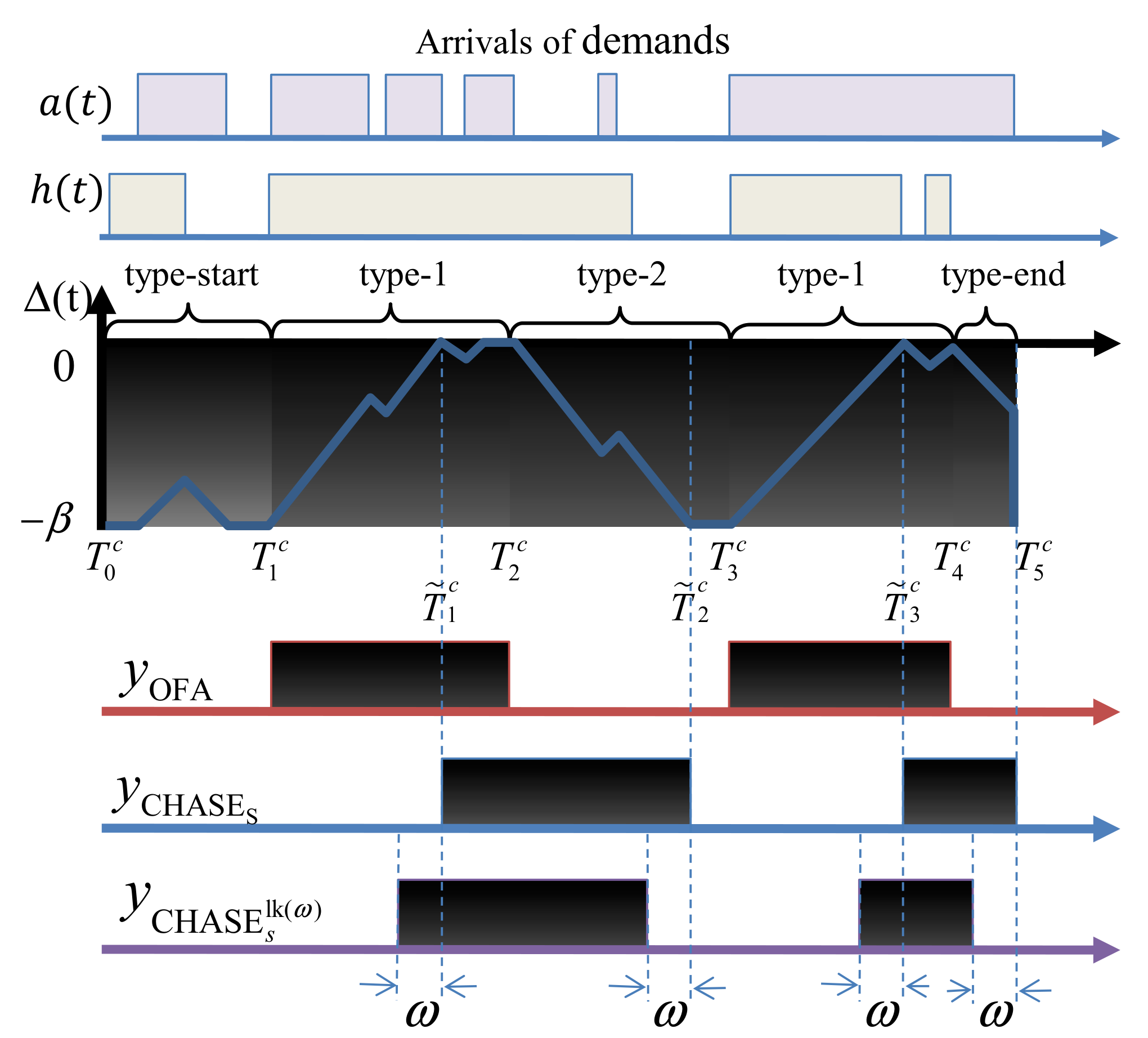
Refer to caption
Figure 3: An example of Δ⁡(t)\Delta(t), yOFA\mathrm{y_{OFA}}, y𝖢𝖧𝖠𝖲𝖤s\mathrm{y_{{\sf CHASE}_{s}}} and y𝖢𝖧𝖠𝖲𝖤slk⁡(ω)\mathrm{y_{{\sf CHASE}_{s}^{lk(\omega)}}}. In the top two rows, we have a⁡(t)∈{0,1}a(t)\in\{0,1\}, h⁡(t)∈{0,η}h(t)\in\{0,\eta\}. The price p⁡(t)p(t) is chosen as a constant in (co−η⋅cg,co)(c_{o}-\eta\cdot c_{g},c_{o}). In the next row, we compute Δ⁡(t)\Delta(t) according to a⁡(t)a(t) and h⁡(t)h(t). For ease of exposition, in this example we set the parameters so that Δ⁡(t)\Delta(t) increases if and only if a⁡(t)=1a(t)=1 and h⁡(t)=ηh(t)=\eta. The solutions yOFA\mathrm{y_{OFA}}, y𝖢𝖧𝖠𝖲𝖤s\mathrm{y_{{\sf CHASE}_{s}}} and y𝖢𝖧𝖠𝖲𝖤slk⁡(ω)\mathrm{y_{{\sf CHASE}_{s}^{lk(\omega)}}} at the bottom rows are obtained accordingly to (8), Algorithms 2 and 4, respectively.

Once the time horizon [1,T][1,T] is divided into critical segments, we can now characterize the optimal solution.

Definition 2.

We classify the type of a critical segment by:

  • •

    type-start (also call type-0): [1,T1c][1,T_{1}^{c}]

  • •

    type-1: [Tic+1,Ti+1c][T_{i}^{c}+1,T_{i+1}^{c}], if Δ⁡(Tic)=−β\Delta(T_{i}^{c})=-\beta and Δ⁡(Ti+1c)=0\Delta(T_{i+1}^{c})=0

  • •

    type-2: [Tic+1,Ti+1c][T_{i}^{c}+1,T_{i+1}^{c}], if Δ⁡(Tic)=0\Delta(T_{i}^{c})=0 and Δ⁡(Ti+1c)=−β\Delta(T_{i+1}^{c})=-\beta

  • •

    type-end (also call type-3): [Tkc+1,T][T_{k}^{c}+1,T]

We define the cost with regard to a segment ii by:

Costsg​-​i​(y)≜∑t=Tic+1Ti+1cψ⁡(σ⁡(t),y⁡(t))+∑t=Tic+1Ti+1c+1β⋅[y⁡(t)−y⁡(t−1)]+\begin{array}[]{@{}r@{}l@{\ }l}{\rm Cost}^{{\rm sg\mbox{-}}i}(y)&\triangleq&{\displaystyle\sum_{t=T_{i}^{c}+1}^{T_{i+1}^{c}}\psi\big(\sigma(t),y(t)\big)}+{\displaystyle\sum_{t=T_{i}^{c}+1}^{T_{i+1}^{c}+1}\beta\cdot[y(t)-y(t-1)]^{+}}\end{array}

and define a subproblem for critical segment ii by:

𝐒𝐏sg​-​i​(yil,yir):min\displaystyle\mathbf{SP}^{{\rm sg\mbox{-}}i}({\rm y}_{i}^{l},{\rm y}_{i}^{r}):\min\; Costsg​-​i​(y)\displaystyle{\rm Cost}^{{\rm sg\mbox{-}}i}(y)
s.t.  y⁡(Tic)=yil,y⁡(Ti+1c+1)=yir,\displaystyle y(T_{i}^{c})={\rm y}_{i}^{l},\;y(T_{i+1}^{c}+1)={\rm y}_{i}^{r},
var  y⁡(t)∈{0,1},t∈[Tic+1,Ti+1c].\displaystyle y(t)\in\{0,1\},t\in[T_{i}^{c}+1,T_{i+1}^{c}].

Note that due to the startup cost across segment boundaries, in general Cost⁡(y)≠∑Costsg​-​i​(y){\rm Cost}(y)\neq\sum{\rm Cost}^{{\rm sg\mbox{-}}i}(y). In other words, we should not expect that putting together the solutions to each segment will lead to an overall optimal offline solution. However, the following lemma shows an important structure property that one optimal solution of 𝐒𝐏𝐬𝐠−𝐢​(yil,yir)\mathbf{SP^{sg-i}}(y_{i}^{l},y_{i}^{r}) is independent of boundary conditions (yil,yir)(y_{i}^{l},y_{i}^{r}) although the optimal value depends on boundary conditions.

Lemma 2

(yOFA​(t))t=Tic+1Ti+1c(y_{{\rm OFA}}(t))_{t=T_{i}^{c}+1}^{T_{i+1}^{c}} in (8) is an optimal solution for 𝐒𝐏sg​-​i​(yil,yir){\bf SP}^{{\rm sg\mbox{-}}i}({\rm y}_{i}^{l},{\rm y}_{i}^{r}), despite any boundary conditions (yil,yir)({\rm y}_{i}^{l},{\rm y}_{i}^{r}).

This lemma can be intuitively explained by Fig. 3. In type-1 critical segment, Δ⁡(t)\Delta(t) has an increment of β\beta, which means that setting y⁡(t)=1y(t)=1 over the entire segment provides at least a benefit of β\beta, compared to keeping y⁡(t)=0y(t)=0. Such benefit compensates the possible startup cost β\beta if the boundary conditions are not aligned with y⁡(t)=1y(t)=1. Therefore, regardless of the boundary conditions, we should set y⁡(t)=1y(t)=1 on type-1 critical segment. Other types of critical segments can be explained similarly.

We then use this lemma to show the following main result on the structure of the offline optimal solution.

Theorem 1.

An optimal solution for SP is given by

yOFA​(t)≜{0,if ​t∈[Tic+1,Ti+1c]​ is type-start/-2/-end,1,if ​t∈[Tic+1,Ti+1c]​ is type-1.y_{{\rm OFA}}(t)\triangleq\begin{cases}0,&\mbox{if\ }t\in[T_{i}^{c}+1,T_{i+1}^{c}]\mbox{\ is type-start/-2/-end},\\ 1,&\mbox{if\ }t\in[T_{i}^{c}+1,T_{i+1}^{c}]\mbox{\ is type-1}.\end{cases} (8)
Proof.

Refer to Appendix A. ∎

Theorem 1 can be interpreted as follows. Consider for example a type-1 critical segment in Fig. 3 that starts from T1cT_{1}^{c}. Since Δ⁡(t)\Delta(t) increases from −β-\beta after T1cT_{1}^{c}, it implies that δ⁡(t)>0\delta(t)>0, and thus we are interested in turning on the generator. The difficulty, however, is that immediately after T1cT_{1}^{c} we do not know whether the future gain by turning on the generator will offset the startup cost. On the other hand, once Δ⁡(t)\Delta(t) reaches 00, it means that the cumulative gain in the interval [T1c,T~1c][T_{1}^{c},\tilde{T}_{1}^{c}] will be no less than the startup cost. Hence, we can safely turn on the generator at T1cT_{1}^{c}. Similarly, for each type-2 segment we can turn off the generator at the beginning of the segment. (We note that our offline solution turns on/off the generator at the beginning of each segment because all future information is assumed to be known.)

The optimal solution is easy to compute. More importantly, the insights help us design the online algorithms.

3.1.2 Our Proposed Online Algorithm 𝖢𝖧𝖠𝖲𝖤{\sf CHASE}

Denote an online algorithm for 𝐒𝐏{\bf SP} by 𝒜{\cal A}. We define the competitive ratio of 𝒜{\cal A} by:

𝖢𝖱⁡(𝒜)≜maxσ⁡Cost⁡(y𝒜)Cost⁡(yOFA){\sf CR}({\cal A})\triangleq\max_{\sigma}\frac{{\rm Cost}(y_{{\cal A}})}{{\rm Cost}(y_{{\rm OFA}})} (9)

Recall the structure of optimal solution yOFAy_{{\rm OFA}}: once the process is entering type-1 (resp., type-2) critical segment, we should set y⁡(t)=1y(t)=1 (resp., y⁡(t)=0y(t)=0). However, the difficulty lies in determining the beginnings of type-1 and type-2 critical segments without future information. Fortunately, as illustrated in Fig. 3, it is certain that the process is in a type-1 critical segment when Δ⁡(t)\Delta(t) reaches 00 for the first time after hitting −β-\beta. This observation motivates us to use the algorithm 𝖢𝖧𝖠𝖲𝖤s{\sf CHASE}_{s}, which is given in Algorithm 2. If −β<Δ⁡(t)<0-\beta<\Delta(t)<0, 𝖢𝖧𝖠𝖲𝖤s{\sf CHASE}_{s} maintains y⁡(t)=y⁡(t−1)y(t)=y(t-1) (since we do not know whether a new segment has started yet.) However, when Δ=0\Delta=0 (resp. Δ⁡(t)=−β\Delta(t)=-\beta), we know for sure that we are inside a new type-1 (resp. type-2) segment. Hence, 𝖢𝖧𝖠𝖲𝖤s{\sf CHASE}_{s} sets y⁡(t)=1y(t)=1 (resp. y⁡(t)=0y(t)=0). Intuitively, the behavior of 𝖢𝖧𝖠𝖲𝖤s{\sf CHASE}_{s} is to track the offline optimal in an online manner: we change the decision only after we are certain that the offline optimal decision is changed.

Algorithm 2 𝖢𝖧𝖠𝖲𝖤s​[t,σ⁡(t),y⁡(t−1)]{\sf CHASE}_{s}[t,\sigma(t),y(t-1)]
1:  find Δ⁡(t)\Delta(t)
2:  if Δ⁡(t)=−β\Delta(t)=-\beta then
3:   y⁡(t)←0y(t)\leftarrow 0
4:  else if Δ⁡(t)=0\Delta(t)=0 then
5:   y⁡(t)←1y(t)\leftarrow 1
6:  else
7:   y⁡(t)←y⁡(t−1)y(t)\leftarrow y(t-1)
8:  end if
9:  set u⁡(t)u(t), v⁡(t)v(t), and s⁡(t)s(t) according to (4) and (5)
10:  return (y⁡(t),u⁡(t),v⁡(t),s⁡(t))(y(t),u(t),v(t),s(t))

Even though 𝖢𝖧𝖠𝖲𝖤s{\sf CHASE}_{s} is a simple algorithm, it has a strong performance guarantee, as given by the following theorem.

Theorem 2.

The competitive ratio of 𝖢𝖧𝖠𝖲𝖤s{\sf CHASE}_{s} satisfies

𝖢𝖱⁡(𝖢𝖧𝖠𝖲𝖤s)≤3−2​α<3,{\sf CR}({\sf CHASE}_{s})\leq 3-2\alpha<3, (10)

where

α≜(co+cm/L)/(Pmax+η⋅cg)∈(0,1]\alpha\triangleq(c_{o}+c_{m}/L)/(P_{\max}+\eta\cdot c_{g})\in(0,1] (11)

captures the maximum price discrepancy between using local generation and external sources to supply energy.

Proof.

Refer to Appendix B. ∎

Remark: (i) The intuition that 𝖢𝖧𝖠𝖲𝖤s{\sf CHASE}_{s} is competitive can be explained by studying its worst case input shown in Fig. 4. The demands and prices are chosen in a way such that in interval [T0c,T1c][T_{0}^{c},T_{1}^{c}] Δ⁡(t)\Delta(t) increases from −β-\beta to 00, and in interval [T1c,T2c][T_{1}^{c},T_{2}^{c}] Δ⁡(t)\Delta(t) decreases from 00 to −β-\beta. We see that in the worst case, y𝖢𝖧𝖠𝖲𝖤sy_{{\sf CHASE}_{s}} never matches y𝖮𝖥𝖠y_{{\sf OFA}}. But even in this worst case, 𝖢𝖧𝖠𝖲𝖤s{{\sf CHASE}_{s}} pays only 2​β2\beta more than the offline solution y𝖮𝖥𝖠{y_{\sf OFA}} on [T0c,T2c][T_{0}^{c},T_{2}^{c}], while y𝖮𝖥𝖠{y_{\sf OFA}} pays at least a startup cost β\beta at time T0cT_{0}^{c}. Hence, the ratio of the online cost over the offline cost cannot be too bad. (ii) Theorem 2 says that 𝖢𝖧𝖠𝖲𝖤s{\sf CHASE}_{s} is more competitive when α\alpha is large than it is small. This can be explained intuitively as follows. Large α\alpha implies small economic advantage of using local generation over external sources to supply energy. Consequently, the offline solution tends to use local generation less. It turns out 𝖢𝖧𝖠𝖲𝖤s{\sf CHASE}_{s} will also use less local generation22 2 𝖢𝖧𝖠𝖲𝖤s{\sf CHASE}_{s} will turn on the local generator when Δ⁡(t)\Delta(t) increases to 0. The larger the α\alpha is, the slower Δ⁡(t)\Delta(t) increases, and the less likely 𝖢𝖧𝖠𝖲𝖤s{\sf CHASE}_{s} will use the local generator. and is competitive to offline solution. Meanwhile, when α\alpha is small, 𝖢𝖧𝖠𝖲𝖤s{\sf CHASE}_{s} starts to use local generation. However, using local generation incurs high risk since we have to pay the startup cost to turn on the generator without knowing whether there are sufficient demands to serve in the future. Lacking future knowledge leads to a large performance discrepancy between 𝖢𝖧𝖠𝖲𝖤s{\sf CHASE}_{s} and the offline optimal solution, making 𝖢𝖧𝖠𝖲𝖤s{\sf CHASE}_{s} less competitive.

Refer to caption
Figure 4: The worst case input of 𝖢𝖧𝖠𝖲𝖤s{{\sf CHASE}_{s}}, and the corresponding y𝖢𝖧𝖠𝖲𝖤𝗌{y_{\sf CHASE_{s}}}, y𝖢𝖧𝖠𝖲𝖤slk⁡(ω)y_{{\sf CHASE}_{s}^{{\rm lk}(\omega)}} and the offline optimal solution y𝖮𝖥𝖠{y_{\sf OFA}}.

The result in Theorem 2 is strong in the sense that 𝖢𝖱⁡(𝖢𝖧𝖠𝖲𝖤s){\sf CR}({\sf CHASE}_{s}) is always upper-bounded by a small constant 3, regardless of system parameters. This is contrast to large parameter-dependent competitive ratios that one can achieve by using generic approach, e.g., the metrical task system framework [8], to design online algorithms. Furthermore, we show that 𝖢𝖧𝖠𝖲𝖤s{\sf CHASE}_{s} achieves close to the best possible competitive ratio for deterministic algorithms as follow.

Theorem 3.

Let ϵ>0\epsilon>0 be the slot length under the discrete-time setting we consider in this paper. The competitive ratio for any deterministic online algorithm 𝒜{\cal A} for 𝐒𝐏{\bf SP} is lower bounded by

𝖢𝖱⁡(𝒜)≥min⁡(3−2​α−o⁡(ϵ),1/α),{\sf CR}({\cal A})\geq\min(3-2\alpha-o(\epsilon),1/\alpha), (12)

where o⁡(ϵ)o(\epsilon) vanishes to zero as ϵ\epsilon goes to zero and the discrete-time setting approaches the continuous-time setting.

Proof.

Refer to Appendix C. ∎

Note that there is still a gap between the competitive ratios in (10) and (12). The difference is due to the term 1/α=(Pmax+η⋅cg)/(co+cm/L)1/\alpha=(P_{\max}+\eta\cdot c_{g})/(c_{o}+c_{m}/L). This term can be interpreted as the competitive ratio of a naive strategy that always uses external power supply and separate heat supply. Intuitively, if this 1/α1/\alpha term is smaller than 3−2​α3-2\alpha, we should simply use this naive strategy. This observation motivates us to develop an improved version of CHASEs\textsf{CHASE}_{s}, called CHASEs+\textsf{CHASE}_{s+}, which is presented in Algorithm 3. Corollary 1 shows that CHASEs+\textsf{CHASE}_{s+} closes the above gap and achieves the asymptotic optimal competitive ratio. Note that whether or not the 1/α1/\alpha term is smaller can be completely determined by the system parameters.

Algorithm 3 𝖢𝖧𝖠𝖲𝖤s+​[t,σ⁡(t),y⁡(t−1)]{\sf CHASE}_{s+}[t,\sigma(t),y(t-1)]
1:  if 1/α≤3−2​α1/\alpha\leq 3-2\alpha then
2:   y⁡(t)←0,u⁡(t)←0,v⁡(t)←a⁡(t),s⁡(t)←h⁡(t)y(t)\leftarrow 0,\ \ u(t)\leftarrow 0,\ \ v(t)\leftarrow a(t),\ \ s(t)\leftarrow h(t)
3:   return (y⁡(t),u⁡(t),v⁡(t),s⁡(t))(y(t),u(t),v(t),s(t))
4:  else
5:   return 𝖢𝖧𝖠𝖲𝖤s​[t,σ⁡(t),y⁡(t−1)]{\sf CHASE}_{s}[t,\sigma(t),y(t-1)]
6:  end if
Corollary 1.

CHASEs+\textsf{CHASE}_{s+} achieves the asymptotic optimal competitive ratio of any deterministic online algorithm, as

𝖢𝖱⁡(𝖢𝖧𝖠𝖲𝖤s+)≤min⁡(3−2​α,1/α).{\sf CR}({\sf CHASE}_{s+})\leq\min(3-2\alpha,1/\alpha). (13)

Remark: At the beginning of Sec. 3.1, we have discussed the structural differences of online server scheduling problems [26, 28] and ours. In what follows, we summarize the solution differences among these problems. Note that we share similar intuitions with [28], both make switching decisions when the penalty cost equals the switching cost. The significant difference, however, is when to reset the penalty counting. In [28], the penalty counting is reset when the demand arrives. In contrast, in our solution, we need to reset the penalty counting only when Δ⁡(t)\Delta(t), given in the non-trivial form in (7), touches 0 or −β-\beta. This particular way of resetting penalty counting is critical for establishing the optimality of our proposed solution. Meanwhile, to compare with [26], the approach in [26] does not explicitly count the penalty. Furthermore, the online server scheduling problem in [26] is formulated as a convex problem, while our problem is a mixed integer problem. Thus, there is no known method to apply the approach in [26] to our problem.

3.2 Look-ahead Setting

We consider the setting where the online algorithm can predict a small window ω\omega of the immediate future. Note that ω=0\omega=0 returns to the case treated in Section 3.1.2, when there is no future information at all. Consider again a type-1 segment [T1c,T2c][T_{1}^{c},T_{2}^{c}] in Fig. 3. Recall that, when there is no future information, the 𝖢𝖧𝖠𝖲𝖤s{\sf CHASE}_{s} algorithm will wait until T~1c\tilde{T}_{1}^{c}, i.e., when Δ⁡(t)\Delta(t) reaches 00, to be certain that the offline solution must turn on the generator. Hence, the 𝖢𝖧𝖠𝖲𝖤s{\sf CHASE}_{s} algorithm will not turn on the generator until this time. Now assume that the online algorithm has the information about the immediate future in a time window of length ω\omega. By the time T~1c−w\tilde{T}_{1}^{c}-w, the online algorithm has already known that Δ⁡(t)\Delta(t) will reach 00 at time T~1c\tilde{T}_{1}^{c}. Hence, the online algorithm can safely turn on the generator at time T~1c−w\tilde{T}_{1}^{c}-w. As a result, the corresponding loss of performance compared to the offline optimal solution is also reduced. Specifically, even for the worst-case input in Fig. 4, there will be some overlap (of length ω\omega) between y𝖢𝖧𝖠𝖲𝖤sy_{{\sf CHASE}_{s}} and y𝖮𝖥𝖠y_{{\sf OFA}} in each segment. Hence, the competitive ratio should also improve with future information. This idea leads to the online algorithm 𝖢𝖧𝖠𝖲𝖤slk⁡(ω){\sf CHASE}_{s}^{{\rm lk}(\omega)}, which is presented in Algorithm 4.

Algorithm 4 𝖢𝖧𝖠𝖲𝖤slk⁡(ω)​[t,(σ⁡(τ))τ=tt+w,y⁡(t−1)]{\sf CHASE}_{s}^{{\rm lk}(\omega)}[t,(\sigma(\tau))_{\tau=t}^{t+w},y(t-1)]
1:  find (Δ⁡(τ))τ=tt+w(\Delta(\tau))_{\tau=t}^{t+w}
2:  set τ′←min{τ=t,…,t+w∣Δ(τ)=0 or =−β}\tau^{\prime}\leftarrow\min\big\{\tau=t,...,t+w\mid\Delta(\tau)=0\mbox{\ or\ }=-\beta\big\}
3:  if Δ⁡(τ′)=−β\Delta(\tau^{\prime})=-\beta then
4:   y⁡(t)←0y(t)\leftarrow 0
5:  else if Δ⁡(τ′)=0\Delta(\tau^{\prime})=0 then
6:   y⁡(t)←1y(t)\leftarrow 1
7:  else
8:   y⁡(t)←y⁡(t−1)y(t)\leftarrow y(t-1)
9:  end if
10:  set u⁡(t)u(t), v⁡(t)v(t), and s⁡(t)s(t) according to (4) and (5)
11:  return (y⁡(t),u⁡(t),v⁡(t),s⁡(t))(y(t),u(t),v(t),s(t))

We can show the following improved competitive ratio when limited future information is available.

Theorem 4.

The competitive ratio of 𝖢𝖧𝖠𝖲𝖤slk⁡(ω){\sf CHASE}_{s}^{{\rm lk}(\omega)} satisfies

𝖢𝖱⁡(𝖢𝖧𝖠𝖲𝖤slk⁡(ω))≤3−2⋅g⁡(α,ω),{\sf CR}\left({\sf CHASE}_{s}^{{\rm lk}(\omega)}\right)\leq 3-2\cdot g\left(\alpha,\omega\right), (14)

where ω≥0\omega\geq 0 is the look-ahead window size, α∈(0,1]\alpha\in(0,1] is defined in (11), and

g⁡(α,ω)=α+(1−α)1+β⁡(L​co+cm/(1−α))/(ω⁡(L​co+cm)​cm).g(\alpha,\omega)=\alpha+\frac{(1-\alpha)}{1+\beta\left(Lc_{o}+c_{m}/(1-\alpha)\right)/\left(\omega(Lc_{o}+c_{m})c_{m}\right)}. (15)

captures the benefit of looking-ahead and monotonically increases from α\alpha to 1 as ω\omega increases. In particular,
𝖢𝖱⁡(𝖢𝖧𝖠𝖲𝖤slk⁡(0))=𝖢𝖱⁡(𝖢𝖧𝖠𝖲𝖤s){\sf CR}({\sf CHASE}_{s}^{{\rm lk}(0)})={\sf CR}({\sf CHASE}_{s}).

Proof.

Refer to Appendix D. ∎

We replace 𝖢𝖧𝖠𝖲𝖤s{\sf CHASE}_{s} by 𝖢𝖧𝖠𝖲𝖤slk⁡(ω){\sf CHASE}_{s}^{{\rm lk}(\omega)} in 𝖢𝖧𝖠𝖲𝖤s+{\sf CHASE}_{s+} and obtain an improved algorithm for the look-ahead setting, named 𝖢𝖧𝖠𝖲𝖤s+lk⁡(ω){\sf CHASE}_{s+}^{{\rm lk}(\omega)}. Fig. 5 shows the competitive ratio of 𝖢𝖧𝖠𝖲𝖤s+lk⁡(ω){\sf CHASE}_{s+}^{{\rm lk}(\omega)} as a function of α\alpha and ω\omega.

Figure 5: The competitive ratio of 𝖢𝖧𝖠𝖲𝖤s+lk⁡(ω){\sf CHASE}_{s+}^{{\rm lk}(\omega)} as a function of α\alpha and ω\omega.

3.3 Multiple Generator Case

Now we consider the general case with NN units of homogeneous generators, each having an maximum power capacity LL, startup cost β\beta, sunk cost cmc_{m} and per unit operational cost coc_{o}. We define a generalized version of problem:

𝐟𝐌𝐂𝐌𝐏:miny,u,v,s\displaystyle\mathbf{fMCMP}:\underset{{y,u,v,s}}{\min} Cost⁡(y,u,v,s)\displaystyle{\rm Cost}(y,u,v,s)
s.t.  Constraints (2b),(2c), and (2d)\displaystyle\mbox{Constraints }\eqref{C_max_output},\;\eqref{C_e-demand},\mbox{ and }\eqref{C_h-demand}
var  yn​(t)∈{0,1},un​(t),v⁡(t),s⁡(t)∈ℝ0+,\displaystyle y_{n}(t)\in\{0,1\},u_{n}(t),v(t),s(t)\in\mathbb{R}_{0}^{+},

Next, we will construct both offline and online solutions to 𝐟𝐌𝐂𝐌𝐏\mathbf{fMCMP} in a divide-and-conquer fashion. We will first partition the demands into sub-demands for each generator, and then optimize the local generation separately for each sub-demand. Note that the key is to correctly partition the demand so that the combined solution is still optimal. Our strategy below essentially slices the demand (as a function of tt) into multiple layers from the bottom up (see Fig. 6). Each layer has at most LL units of electricity demand and η⋅L\eta\cdot L units of heat demand. The intuition here is that the layers at the bottom exhibit the least frequent variations of demand. Hence, by assigning each of the layers at the bottom to a dedicated generator, these generators will incur the least amount of switching, which helps to reduce the startup cost.

More specifically, given (a⁡(t),h⁡(t))(a(t),h(t)), we slice them into N+1N+1 layers:

aly​-​1​(t)=\displaystyle a^{{\rm ly\mbox{-}}1}(t)= min⁡{L,a⁡(t)},hly​-​1​(t)=min⁡{η⋅L,h⁡(t)}\displaystyle\min\{L,a(t)\},\quad h^{{\rm ly\mbox{-}}1}(t)=\min\{\eta\cdot L,h(t)\} (16a)
aly​-​n​(t)=\displaystyle a^{{\rm ly\mbox{-}}n}(t)= min⁡{L,a⁡(t)​-​∑r=1n−1aly​-​r​(t)},n∈[2,N]\displaystyle\min\{L,a(t)\mbox{-}\textstyle{\sum}_{r=1}^{n-1}a^{{\rm ly\mbox{-}}r}(t)\},n\in[2,N] (16b)
hly​-​n​(t)=\displaystyle h^{{\rm ly\mbox{-}}n}(t)= min⁡{η⋅L,h⁡(t)​-​∑r=1n−1hly​-​r​(t)},n∈[2,N]\displaystyle\min\{\eta\cdot L,h(t)\mbox{-}\textstyle{\sum}_{r=1}^{n-1}h^{{\rm ly\mbox{-}}r}(t)\},n\in[2,N] (16c)
atop​(t)=\displaystyle a^{\rm top}(t)= min⁡{L,a⁡(t)−∑r=1Naly​-​r​(t)}\displaystyle\min\{L,a(t)-\textstyle{\sum}_{r=1}^{N}a^{{\rm ly\mbox{-}}r}(t)\} (16d)
htop​(t)=\displaystyle h^{\rm top}(t)= min⁡{η⋅L,h⁡(t)−∑r=1Nhly​-​r​(t)}\displaystyle\min\{\eta\cdot L,h(t)-\textstyle{\sum}_{r=1}^{N}h^{{\rm ly\mbox{-}}r}(t)\} (16e)
Refer to caption
(a) An example of (aly−n)(a^{\mathrm{ly-n}}).
Refer to caption
(b) An example of (hly−n)(h^{\mathrm{ly-n}}).
Figure 6: An example of (aly−n)(a^{\mathrm{ly-n}}) and (hly−n)(h^{\mathrm{ly-n}}). In this example, N=2.N=2. We obtain 33 layers of electricity and heat demands, respectively.

It is easy to see that electricity demand satisfies aly​-​n​(t)≤La^{{\rm ly\mbox{-}}n}(t)\leq L and heat demand satisfies hly​-​n​(t)≤η⋅Lh^{{\rm ly\mbox{-}}n}(t)\leq\eta\cdot L. Thus, each layer of sub-demand can be served by a single local generator if needed. Note that (atop,htop)(a^{\rm top},h^{\rm top}) can only be satisfied from external supplies, because they exceed the capacity of local generation.

Based on this decomposition of demand, we then decompose the fMCMP problem into NN sub-problems fMCMPsly​-​n\textbf{fMCMP}_{\rm s}^{{\rm ly\mbox{-}}n} (1≤n≤N1\leq n\leq N), each of which is an fMCMPs\textbf{fMCMP}_{\rm s} problem with input (aly​-​n,hly​-​n,p)(a^{{\rm ly\mbox{-}}n},h^{{\rm ly\mbox{-}}n},p). We then apply the offline and online algorithms developed earlier to solve each sub-problem fMCMPsly​-​n\textbf{fMCMP}_{\rm s}^{{\rm ly\mbox{-}}n} (1≤n≤N1\leq n\leq N) separately. By combining the solutions to these sub-problems, we obtain offline and online solutions to fMCMP. For the offline solution, the following theorem states that such a divide-and-conquer approach results in no optimality loss.

Theorem 5.

Suppose (yn,un,vn,sn)(y_{n},u_{n},v_{n},s_{n}) is an optimal offline solution for each fMCMPsly​-​n\textbf{fMCMP}_{\rm s}^{{\rm ly\mbox{-}}n} (1≤n≤N1\leq n\leq N). Then
((yn∗,un∗)n=1N,v∗,s∗)((y^{\ast}_{n},u^{\ast}_{n})_{n=1}^{N},v^{\ast},s^{\ast}) defined as follows is an optimal offline solution for fMCMP:

yn∗​(t)=yn​(t),v∗​(t)=atop​(t)+∑n=1Nvn​(t)un∗​(t)=un​(t),s∗​(t)=htop​(t)+∑n=1Nsn​(t)\begin{array}[]{@{}r@{\ }r@{\ }l@{}}y^{\ast}_{n}(t)&=&y_{n}(t),\ \ v^{\ast}(t)=a^{\rm top}(t)+\sum_{n=1}^{N}v_{n}(t)\\ u^{\ast}_{n}(t)&=&u_{n}(t),\ \ s^{\ast}(t)=h^{\rm top}(t)+\sum_{n=1}^{N}s_{n}(t)\end{array} (17)
Proof.

Refer to Appendix E. ∎

For the online solution, we also apply such a divide-and-conquer approach by using (i) a central demand dispatching module that slices and dispatches demands to individual generators according to (16a)-(16e), and (ii) an online generation scheduling module sitting on each generator nn (1≤n≤N1\leq n\leq N) independently solving their own fMCMPsly​-​n\textbf{fMCMP}_{s}^{{\rm ly\mbox{-}}n} sub-problem using the online algorithm 𝖢𝖧𝖠𝖲𝖤s+lk⁡(ω){\sf CHASE}_{s+}^{\rm lk(\omega)}.

The overall online algorithm, named 𝖢𝖧𝖠𝖲𝖤lk⁡(ω){\sf CHASE}^{\rm lk(\omega)}, is simple to implement without the need to coordinate the control among multiple local generators. Since the offline (resp. online) cost of fMCMP is the sum of the offline (resp. online) costs of fMCMPsly​-​n\textbf{fMCMP}_{s}^{{\rm ly\mbox{-}}n} (1≤n≤N1\leq n\leq N), it is not difficult to establish the competitive ratio of 𝖢𝖧𝖠𝖲𝖤lk⁡(ω){\sf CHASE}^{\rm lk(\omega)} as follows.

Theorem 6.

The competitive ratio of 𝖢𝖧𝖠𝖲𝖤lk⁡(ω){\sf CHASE}^{\rm lk(\omega)} satisfies

𝖢𝖱⁡(𝖢𝖧𝖠𝖲𝖤lk⁡(ω))≤min⁡(3−2⋅g⁡(α,ω),1/α),{\sf CR}({\sf CHASE}^{\rm lk(\omega)})\leq\min(3-2\cdot g(\alpha,\omega),1/\alpha), (18)

where α∈(0,1]\alpha\in(0,1] is defined in (11) and g⁡(α,ω)∈[α,1]g(\alpha,\omega)\in[\alpha,1] is defined in (15).

Proof.

Refer to Appendix F. ∎

4 Slow-responding Generator Case

We next consider the slow-responding generator case, with the generators having non-negligible constraints on the minimum on/off periods and the ramp-up/down speeds. For this slow-responding version of MCMP, its offline optimal solution is harder to characterize than fMCMP due to the additional challenges introduced by the cross-slot constraints (2e)-(2h).

In the slow-responding setting, local generators cannot be turned on and off immediately when demand changes. Rather, if a generator is turned on (resp., off) at time tt, it must remain on for at least 𝖳on{\sf T}_{{\rm on}} (resp., 𝖳off{\sf T}_{{\rm off}}) time . Further, the changes of un​(t)−un​(t−1)u_{n}(t)-u_{n}(t-1) must be bounded by 𝖱up{\sf R}_{{\rm up}} and −𝖱down-{\sf R}_{{\rm down}}.

A simple heuristic is to first compute solutions based on 𝖢𝖧𝖠𝖲𝖤lk⁡(ω){\sf CHASE}^{\rm lk(\omega)}, and then modify the solutions to respect the above constraints. We name this heuristic 𝖢𝖧𝖠𝖲𝖤genlk⁡(ω){\sf CHASE}^{\rm lk(\omega)}_{\rm gen} and present it in Algorithm  5. For simplicity, Algorithm  5 is a single-generator version, which can be easily extended to the multiple-generator scenario by following the divide-and-conquer approach elaborated in Sec. 3.3.

Algorithm 5 𝖢𝖧𝖠𝖲𝖤genlk⁡(ω)​[t,(σ⁡(τ))τ=1t+ω,y⁡(t−1)]{\sf CHASE}^{\rm lk(\omega)}_{\rm gen}[t,(\sigma(\tau))_{\tau=1}^{t+\omega},y(t-1)]
1:  (ys​(t),us​(t),vs​(t),ss​(t))←𝖢𝖧𝖠𝖲𝖤slk⁡(ω)​[t,(σ⁡(τ))τ=1t+w,y⁡(t​-​1)]\big(y_{s}(t),u_{s}(t),v_{s}(t),s_{s}(t)\big)\leftarrow{\sf CHASE}_{s}^{{\rm lk}(\omega)}\big[t,\big(\sigma\big(\tau\big)\big)_{\tau=1}^{t+w},y\big(t\mbox{-}1\big)\big]
2:  if y(τ1)≤1−𝟏{ys(t)>y(t−1)},∀τ1∈[max(1,t−𝖳off),t−1]y(\tau_{1})\leq 1-\mathbf{1}_{\{y_{s}(t)>y(t-1)\}},\ \forall\tau_{1}\in[\max(1,t-{\sf T}_{{\rm off}}),t-1] and y(τ2)≥𝟏{ys(t)<y(t−1)},∀τ2∈[max(1,t−𝖳on),t−1]y(\tau_{2})\geq\mathbf{1}_{\{y_{s}(t)<y(t-1)\}},\ \forall\tau_{2}\in[\max(1,t-{\sf T}_{{\rm on}}),t-1] then
3:   y​(t)←ys​(t)y(t)\leftarrow y_{s}(t)
4:  else
5:   y⁡(t)←y⁡(t−1)y(t)\leftarrow y(t-1)
6:  end if
7:  if us​(t)>u⁡(t−1)u_{s}(t)>u(t-1) then
8:   u⁡(t)←u⁡(t−1)+min⁡(𝖱up,us​(t)−u⁡(t−1))u(t)\leftarrow u(t-1)+\min\big({\sf R}_{{\rm up}},u_{s}(t)-u(t-1)\big)
9:  else
10:   u⁡(t)←u⁡(t−1)−min⁡(𝖱dw,u⁡(t−1)−us​(t))u(t)\leftarrow u(t-1)-\min\big({\sf R}_{{\rm dw}},u(t-1)-u_{s}(t)\big)
11:  end if
12:  v⁡(t)←[a⁡(t)−u⁡(t)]+{v(t)\leftarrow\big[a(t)-u(t)\big]^{+}}
13:  s⁡(t)←[h⁡(t)−η⋅u⁡(t)]+{s(t)\leftarrow\big[h(t)-\eta\cdot u(t)\big]^{+}}
14:  return (y⁡(t),u⁡(t),v⁡(t),s⁡(t))\big(y(t),u(t),v(t),s(t)\big)

We now explain Algorithm 5 and its competitive ratio. At each time slot tt, we obtain the solution of 𝖢𝖧𝖠𝖲𝖤slk⁡(ω){\sf CHASE}_{s}^{{\rm lk}(\omega)}, including ys​(t),us​(t),vs​(t),ss​(t)y_{s}(t),u_{s}(t),v_{s}(t),s_{s}(t), as a reference solution (Line 1). Then in Line 2-6, we modify the reference solution’s ys​(t)y_{s}(t) to our actual solution y⁡(t)y(t), to respect the constraints of minimum on/off periods. More specifically, we follow the reference solution’s ys​(t)y_{s}(t) (i.e., y​(t)=ys​(t)y(t)=y_{s}(t)) if and only if it respects the minimum on/off periods constraints (Line 2-3). Otherwise, we let our actual solution’s y⁡(t)y(t) equal our previous slot’s solution (y⁡(t)=y⁡(t−1)y(t)=y(t-1)) (Line 4-5). Similarly, we modify the reference solution’s us​(t)u_{s}(t) to our actual solution’s u⁡(t)u(t), to respect the constraints on ramp-up/down speeds (Line 7-11). At last, in our actual solution, we use (v⁡(t),s⁡(t))(v(t),s(t)) to compensate the supply and satisfy the demands (Line 12-13). In summary, our actual solution is designed to be aligned with the reference solution as much as possible. We derive an upper bound on the competitive ratio of 𝖢𝖧𝖠𝖲𝖤genlk⁡(ω){\sf CHASE}^{\rm lk(\omega)}_{\rm gen} as follows.

Theorem 7.

The competitive ratio of 𝖢𝖧𝖠𝖲𝖤genlk⁡(ω)\mathrm{{\sf CHASE}_{\rm gen}^{{\rm lk}(\omega)}} is upper bounded by (3−2​g​(α,ω))⋅max⁡(r1,r2)(3-2g(\alpha,\omega))\cdot\max\big(r_{1},r_{2}\big), where g⁡(α,ω)g(\alpha,\omega) is defined in (15) and

r1=\displaystyle r_{1}= 1+max{(Pmax+cg⋅η−c0)L​c0+cmmax{0,(L−𝖱up)}\displaystyle 1+\max\left\{\frac{\big(P_{\max}+c_{g}\cdot\eta-c_{0}\big)}{Lc_{0}+c_{m}}\max\left\{0,\big(L-{\sf R}_{{\rm up}}\big)\right\}\right.
cocmmax{0,(L−𝖱dw)}},\displaystyle\left.\frac{c_{o}}{c_{m}}\max\left\{0,\big(L-{\sf R}_{{\rm dw}}\big)\right\}\right\},
and ​r2=\displaystyle\mbox{and }r_{2}= β+cm⋅𝖳onβ+L⁡(Pmax+cg⋅η)β​(𝖳on+𝖳off).\displaystyle\frac{\beta+c_{m}\cdot{\sf T}_{{\rm on}}}{\beta}+\frac{L\big(P_{\max}+c_{g}\cdot\eta\big)}{\beta}\left({\sf T}_{{\rm on}}+{\sf T}_{{\rm off}}\right).
Proof.

Refer to Appendix G. ∎

We note that when 𝖳on=𝖳off=0{\sf T}_{{\rm on}}={\sf T}_{{\rm off}}=0, 𝖱up=𝖱dw=∞{\sf R}_{{\rm up}}={\sf R}_{{\rm dw}}=\infty, the above upper bound matches that of 𝖢𝖧𝖠𝖲𝖤lk⁡(ω){\sf CHASE}^{\rm lk(\omega)} in Theorem 6 (specifically the first term inside the min function).

5 Empirical Evaluations

We evaluate the performance of our algorithms based on evaluations using real-world traces. Our objectives are three-fold: (i) evaluating the potential benefits of CHP and the ability of our algorithms to unleash such potential, (ii) corroborating the empirical performance of our online algorithms under various realistic settings, and (iii) understanding how much local generation to invest to achieve substantial economic benefit.

5.1 Parameters and Settings

Demand Trace: We obtain the demand traces from California Commercial End-Use Survey (CEUS) [1]. We focus on a college in San Francisco, which consumes about 154 GWh electricity and 5.1×1065.1\times 10^{6} therms gas per year. The traces contain hourly electricity and heat demands of the college for year 2002. The heat demands for a typical week in summer and spring are shown in Fig. 7. They display regular daily patterns in peak and off-peak hours, and typical weekday and weekend variations.

Wind Power Trace: We obtain the wind power traces from [4]. We employ power output data for the typical weeks in summer and spring with a resolution of 1 hour of an offshore wind farm right outside San Francisco with an installed capacity of 12MW. The net electricity demand, which is computed by subtracting the wind generation from electricity demand is shown in Fig. 7. The highly fluctuating and unpredictable nature of wind generation makes it difficult for the conventional prediction-based energy generation scheduling solutions to work effectively.

Electricity and Natural Gas Prices: The electricity and natural gas price data are from PG&E [5] and are shown in Table 3. Besides, the grid electricity prices for a typical week in summer and winter are shown in Fig. 7. Both the electricity demand and the price show strong diurnal properties: in the daytime, the demand and price are relatively high; at nights, both are low. This suggests the feasibility of reducing the microgrid operating cost by generating cheaper energy locally to serve the demand during the daytime when both the demand and electricity price are high.

Generator Model: We adopt generators with specifications the same as the one in [6]. The full output of a single generator is L=3​M​WL=3MW. The incremental cost per unit time to generate an additional unit of energy coc_{o} is set to be 0.051/K​W​h0.051/KWh, which is calculated according to the natural gas price and the generator efficiency. We set the heat recovery efficiency of co-generation η\eta to be 1.81.8 according to [6]. We also set the unit-time generator running cost to be cm=110$/hc_{m}=110\$/h, which includes the amortized capital cost and maintenance cost according to a similar setting from [36]. We set the startup cost β\beta equivalent to running the generator at its full capacity for about 5 hrs at its own operating cost which gives β=1400$\beta=1400\$. In addition, we assume for each generator 𝖳on=𝖳off=3​h{\sf T}_{{\rm on}}={\sf T}_{{\rm off}}=3h and 𝖱up=𝖱dw=1​M​W/h{\sf R}_{{\rm up}}={\sf R}_{{\rm dw}}=1MW/h, unless mentioned otherwise. For electricity demand trace we use, the peak demand is 30MW. Thus, we assume there are 10 such CHP generators so as to fully satisfy the demand.

Local Heating System: We assume an on-demand heating system with capacity sufficiently large to satisfy all the heat demand by itself and without on-off cost or ramp limit. The efficiency of a heating system is set to 0.80.8 according to [2], and consequently we can compute the unit heat generation cost to be cg=0.0179$/KWhc_{g}=0.0179\$/KWh.

Cost Benchmark: We use the cost incurred by using only external electricity, heating and wind energy (without CHP generators) as a benchmark. We evaluate the cost reduction due to our algorithms.

Comparisons of Algorithms: We compare three algorithms in our simulations. (1) our online algorithm CHASE; (2) the Receding Horizon Control (RHC) algorithm; and (3) the OFFLINE optimal algorithm we introduce in Sec. 4. RHC is a heuristic algorithm commonly used in the control literature [23]. In RHC, an estimate of the near future (e.g., in a window of length ww) is used to compute a tentative control trajectory that minimizes the cost over this time-window. However, only the first step of this trajectory is implemented. In the next time slot, the window of future estimates shifts forward by 11 slot. Then, another control trajectory is computed based on the new future information, and again only the first step is implemented. This process then continues. We note that because at each step RHC does not consider any adversarial future dynamics beyond the time-window ww, there is no guarantee that RHC is competitive. For the OFFLINE algorithm, the inputs are system parameters (such as β\beta, cmc_{m} and 𝖳on{\sf T}_{{\rm on}}), electricity demand, heat demand, wind power output, gas price, and grid electricity price. For online algorithms CHASE and RHC, the input is the same as the OFFLINE except that at time tt, only the demands, wind power output, and prices in the past and the look-ahead window (i.e., [1,t+w][1,t+w]) are available. The output for all three algorithms is the total cost incurred during the time horizon [1,T][1,T].

(a) Summer
(b) Winter
Figure 7: Electricity net demand and heat demand for a typical week in summer and winter. The net demand is computed by subtracting the wind generation from the electricity demand. The net electricity demand and the heat demand need to be satisfied by using the local CHP generators, the electricity grid, and the heating system.
Electricity Summer (May-Oct.) Winter (Nov.-Apr.)
$/kWh $/kWh
On-peak 0.232 N/A
Mid-peak 0.103 0.116
Off-peak 0.056 0.072
Natural Gas 0.419$/therm 0.486$/therm
Table 3: PG&E commercial tariffs and natural gas tariffs. In the table, summer on-peak, mid-peak, and off-peak hours are weekday 12-18, weekday 8-12, and the remaining hours, respectively. Winter mid-peak and off-peak hours are weekday 8-22 and the remaining hours, respectively. The gas price is an average; monthly prices vary slightly according to PG&E.

5.2 Potential Benefits of CHP

Purpose: The experiments in this subsection aim to answer two questions. First, what is the potential savings with microgrids? Note that electricity, heat demand, wind station output as well as energy price all exhibit seasonal patterns. As we can see from Figs. 7a and 7b, during summer (similarly autumn) the electricity price is high, while during winter (similarly spring) the heat demand is high. It is then interesting to evaluate under what settings and inputs the savings will be higher. Second, what is the difference in cost-savings with and without the co-generation capability? In particular, we conduct two sets of experiments to evaluate the cost reductions of various algorithms. Both experiments have the same default settings, except that the first set of experiments (referred to as CHP) assumes the CHP technology in the generators is enabled, and the second set of experiments (referred to as NOCHP) assumes the CHP technology is not available, in which case the heat demand must be satisfied solely by the heating system. In all experiments, the look-ahead window size is set to be w=3w=3 hours according to power system operation and wind generation forecast practice [3]. The cost reductions of different algorithms are shown in Fig. 8a and 8b. The vertical axis is the cost reduction as compared to the cost benchmark presented in Sec. 5.1.

Observations: First, the whole-year cost reductions obtained by OFFLINE are 21.8% and 11.3% for CHP and NOCHP scenarios, respectively. This justifies the economic potential of using local generation, especially when CHP technology is enabled. Then, looking at the seasonal performance of OFFLINE, we observe that OFFLINE achieves much more cost savings during summer and autumn than during spring and winter. This is because the electricity price during summer and autumn is very high, thus we can benefit much more from using the relatively-cheaper local generation as compared to using grid energy only. Moreover, OFFLINE achieves much more cost savings when CHP is enabled than when it is not during spring and winter. This is because, during spring and winter, the electricity price is relatively low and the heat demand is high. Hence, just using local generation to supply electricity is not economical. Rather, local generation becomes more economical only if it can be used to supply both electricity and heat together (i.e., with CHP technology).

Second, CHASE performs consistently close to OFFLINE across inputs from different seasons, even though the different settings have very different characteristics of demand and supply. In contrast, the performance of RHC depends heavily on the input characteristics. For example, RHC achieves some cost reduction during summer and autumn when CHP is enabled, but achieves 0 cost reduction in all the other cases.

Ramifications: In summary, our experiments suggest that exploiting local generation can save more cost when the electricity price is high, and CHP technology is more critical for cost reduction when heat demand is high. Regardless of the problem setting, it is important to adopt an intelligent online algorithm (like CHASE) to schedule energy generation, in order to realize the full benefit of microgrids.

(a) Local generators with CHP
(b) Local generators without CHP
Figure 8: Cost reductions for different seasons and the whole year.

5.3 Benefits of Looking-Ahead

Purpose: We compare the performances of CHASE to RHC and OFFLINE for different sizes of the look-ahead window and show the results in Fig. 10. The vertical axis is the cost reduction as compared to the cost benchmark in Sec. 5.1 and the horizontal axis is the size of lookahead window, which varies from 0 to 20 hours.

Observations: We observe that the performance of our online algorithm CHASE is already close to OFFLINE even when no or little look-ahead information is available (e.g., w=0w=0, 11, and 22). In contrast, RHC performs poorly when the look-ahead window is small. When ww is large, both CHASE and RHC perform very well and their performance are close to OFFLINE when the look-ahead window ww is larger than 15 hours.

An interesting observation is that it is more important to perform intelligent energy generation scheduling when there is no or little look-ahead information available. When there are abundant look-ahead information available, both CHASE and RHC achieve good performance and it is less critical to carry out sophisticated algorithm design.

In Fig. 11a and 11b, we separately evaluate the benefit of looking-ahead under the fast-responding and slow-responding scenarios. We evaluate the empirical competitive ratio between the cost of CHASE and OFFLINE, and compare it with the theoretical competitive ratio according to our analytical results. In the fast-responding scenario (Fig. 11a), for each generator there are no minimum on/off period and ramping-up/down constraints. Namely, 𝖳on=0{\sf T}_{{\rm on}}=0, 𝖳off=0{\sf T}_{{\rm off}}=0, 𝖱up=∞{\sf R}_{{\rm up}}=\infty, 𝖱dw=∞{\sf R}_{{\rm dw}}=\infty. In the slow-responding scenario (Fig. 11b), we set 𝖳on=𝖳off=3​h{\sf T}_{{\rm on}}={\sf T}_{{\rm off}}=3h and 𝖱up=𝖱dw=1​M​W/h{\sf R}_{{\rm up}}={\sf R}_{{\rm dw}}=1MW/h. In both experiments, we observe that the theoretical ratio decreases rapidly as look-ahead window size increases. Further, the empirical ratio is already close to one even when there is no look-ahead information.

Figure 9: Cost reduction as a function of look ahead window size ω\omega.
Figure 10: Cost reduction as a function of local generation capacity.
(a) Fast-responding scenario
(b) Slow-responding scenario
Figure 11: Theoretical and empirical ratios for CHASE, as functions of look-ahead window size ω\omega. Note that the theoretical competitive ratios (or their bounds) measure the worst-case performance and are often much larger than the empirical ratios observed in practice.

5.4 Impacts of Look-ahead Error

Purpose: Previous experiments show that our algorithms have better performance if a larger time-window of accurate look-ahead input information is available. The input information in the look-ahead window includes the wind station power output, the electricity and heat demand, and the central grid electricity price. In practice, these look-ahead information can be obtained by applying sophisticated prediction techniques based on the historical data. However, there are always prediction errors. For example, while the day-ahead electricity demand can be predicted within 2-3% range, the wind power prediction in the next hours usually comes with an error range of 20-50% [20]. Therefore, it is important to evaluate the performance of the algorithms in the presence of prediction error.

Observations: To achieve this goal, we evaluate CHASE with look-ahead window size of 1 and 3 hours. According to [20], the hour-level wind-power prediction-error in terms of the percentage of the total installed capacity usually follows Gaussian distribution. Thus, in the look-ahead window, a zero-mean Gaussian prediction error is added to the amount of wind power in each time-slot. We vary the standard deviation of the Gaussian prediction error from 0 to 120% of the total installed capacity. Similarly, a zero-mean Gaussian prediction error is added to the heat demand, and its standard deviation also varies from 0 to 120% of the peak demand. We note that in practice, prediction errors are often in the range of 20-50% for 3-hour prediction [20]. Thus, by using a standard deviation up to 120%, we are essentially stress-testing our proposed algorithms. We average 20 runs for each algorithm and show the results in Figs. 12a and 12b. As we can see, both CHASE and RHC are fairly robust to the prediction error and both are more sensitive to the wind-power prediction error than to the heat-demand prediction error. Besides, the impact of the prediction error is relatively small when the look-ahead window size is small, which matches with our intuition.

(a) Wind power forecast error
(b) Heat demand forecast error
Figure 12: Cost reduction as a function of the size prediction error (measured by the standard deviation of the prediction error as a percentage of (a)installed capacity and (b)peak heat demand).

5.5 Impacts of System Parameters

Purpose: Microgrids may employ different types of local generators with diverse operational constraints (such ramping up/down limits and minimum on/off times) and heat recovery efficiencies. It is then important to understand the impact on cost reduction due to these parameters. In this experiment, we study the cost reduction provided by our offline and online algorithms under different settings of 𝖱up{\sf R}_{{\rm up}}, 𝖱dw{\sf R}_{{\rm dw}} , 𝖳on{\sf T}_{{\rm on}}, 𝖳off{\sf T}_{{\rm off}} and η\eta.

Observations: Fig. 13a and 13b show the impact of ramp limit and minimum on/off time, respectively, on the performance of the algorithms. Note that for simplicity we always set 𝖱up=𝖱dw{\sf R}_{{\rm up}}={\sf R}_{{\rm dw}} and 𝖳on=𝖳off{\sf T}_{{\rm on}}={\sf T}_{{\rm off}}. As we can see in Fig. 13a, with 𝖱up{\sf R}_{{\rm up}} and 𝖱dw{\sf R}_{{\rm dw}} of about 40% of the maximum capacity, CHASE obtains nearly all of the cost reduction benefits, compared with 𝖱𝖧𝖢{\sf RHC} which needs 70% of the maximum capacity. Meanwhile, it can be seen from Fig. 13b that 𝖳on{\sf T}_{{\rm on}} and 𝖳off{\sf T}_{{\rm off}} do not have much impact on the performance. This suggests that it is more valuable to invest in generators with fast ramping up/down capability than those with small minimum on/off periods. From Fig. 13c and 13d, we observe that generators with large η\eta save much more cost during the winter because of the high heat demand. This suggests that in areas with large heat demand, such as Alaska and Washington, the heat recovery efficiency ratio is a critical parameter when investing CHP generators.

(a) cost redu. vs. 𝖱up{\sf R}_{{\rm up}} and 𝖱dw{\sf R}_{{\rm dw}}
(b) cost redu. vs. 𝖳up{\sf T}_{{\rm up}} and 𝖳dw{\sf T}_{{\rm dw}}
(c) cost reduction vs. η\eta
(d) cost reduction vs. η\eta
Figure 13: Cost reduction as functions of generator parameters.

5.6 How Much Local Generation is Enough

Thus far, we assumed that the microgrid had the ability to supply all energy demand from local power generation in every time-slot. In practice, local generators can be quite expensive. Hence, an important question is how much investment should a microgrid operator makes (in terms of the installed local generator capacity) in order to obtain the maximum cost benefit. More specifically, we vary the number of CHP generators from 1 to 10 and plot the corresponding cost reductions of algorithms in Fig. 10. Interestingly, our results show that provisioning local generation to produce 60% of the peak demand is sufficient to obtain nearly all of the cost reduction benefits. Further, with just 50% local generation capacity we can achieve about 90% of the maximum cost reduction. The intuitive reason is that most of the time demands are significantly lower than their peaks.

6 Related Work

Energy generation scheduling is a classical problem in power systems and involves two aspects, namely Unit Commitment (UC) and Economic Dispatching (ED). UC optimizes the startup and shutdown schedule of power generations to meet the forecasted demand over a short period, whereas ED allocates the system demand and spinning reserve capacity among operating units at each specific hour of operation without considering startup and shutdown of power generators.

For large power systems, UC involves scheduling of a large number gigantic power plants of several hundred if not thousands of megawatts with heterogeneous operating constraints and logistics behind each action [34]. The problem is very challenging to solve and has been shown to be NP-Complete in general33 3 We note that 𝐟𝐌𝐂𝐌𝐏\mathbf{fMCMP} in (3a)-(3d) is an instance of UC, and that UC is NP-hard in general does not imply that the instance 𝐟𝐌𝐂𝐌𝐏\mathbf{fMCMP} is also NP-hard. [16]. Sophisticated approaches proposed in the literature for solving UC include mixed integer programming [10], dynamic programming [35], and stochastic programming [37]. There have also been investigations on UC with high renewable energy penetration [38], based on over-provisioning approach. After UC determines the on/off status of generators, ED computes their output levels by solving a nonlinear optimization problem using various heuristics without altering the on/off status of generators [14]. There is also recent interest in involving CHP generators in ED to satisfy both electricity and heat demand simultaneously [17]. See comprehensive surveys on UC in [34] and on ED in [14].

However, these studies assume the demand and energy supply (or their distributions) in the entire time horizon are known a prior. As such, the schemes are not readily applicable to microgrid scenarios where accurate prediction of small-scale demand and wind power generation is difficult to obtain due to limited management resources and their unpredictable nature [42].

Several recent works have started to study energy generation strategies for microgrids. For example, the authors in [18] develop a linear programming based cost minimization approach for UC in microgrids. [19] considers the fuel consumption rate minimization in microgrids and advocates to build ICT infrastructure in microgrids. [25, 27] discuss the energy scheduling problems in data centers, whose models are similar with ours. The difference between these works and ours is that they assume the demand and energy supply are given beforehand, and ours does not rely on input prediction.

Online optimization and algorithm design is an established approach in optimizing the performance of various computer systems with minimum knowledge of inputs [8, 32]. Recently, it has found new applications in data centers [15, 9, 39, 26, 28, 29]. To the best of our knowledge, our work is the first to study the competitive online algorithms for energy generation in microgrids with intermittent energy sources and co-generation. The authors in [31] apply online convex optimization framework [43] to design ED algorithms for microgrids. The authors in [21] adopt Lyapunov optimization framework [32] to design electricity scheduling for microgrids, with consideration of energy storage. However, neither of the above considers the startup cost of the local generations. In contrast, our work jointly consider UC and ED in microgrids with co-generation. Furthermore, the above three works adopt different frameworks and provide online algorithms with different types of performance guarantee.

7 Conclusion

In this paper, we study online algorithms for the micro-grid generation scheduling problem with intermittent renewable energy sources and co-generation, with the goal of maximizing the cost-savings with local generation. Based on insights from the structure of the offline optimal solution, we propose a class of competitive online algorithms, called CHASE that track the offline optimal in an online fashion. Under typical settings, we show that CHASE achieves the best competitive ratio of all deterministic online algorithms, and the ratio is no larger than a small constant 3. We also extend our algorithms to intelligently leverage on limited prediction of the future, such as near-term demand or wind forecast. By extensive empirical evaluations using real-world traces, we show that our proposed algorithms can achieve near offline-optimal performance.

There are a number of interesting directions for future work. First, energy storage systems (e.g., large-capacity battery) have been proposed as an alternate approach to reduce energy generation cost (during peak hours) and to integrate renewable energy sources. It would be interesting to study whether our proposed microgrid control strategies can be combined with energy storage systems to further reduce generation cost. However, current energy storage systems can be very expensive. Hence, it is critical to study whether the combined control strategy can reduce sufficient cost with limited amount of energy storage. Second, it remains an open issue whether CHASE can achieve the best competitive ratios in general cases (e.g., in the slow-responding case).

8 Acknowledgments

The work described in this paper was partially supported by China National 973 projects (No. 2012CB315904 and 2013CB336700), several grants from the University Grants Committee of the Hong Kong Special Administrative Region, China (Area of Excellence Project No. AoE/E-02/08 and General Research Fund Project No. 411010 and 411011), two gift grants from Microsoft and Cisco, and Masdar Institute-MIT Collaborative Research Project No. 11CAMA1. Xiaojun Lin would like to thank the Institute of Network Coding at The Chinese University of Hong Kong for the support of his sabbatical visit, during which some parts of the work were done.

References

  • [1] California commercial end-use survey. Internet:http://capabilities.itron.com/CeusWeb/.
  • [2] Green energy. Internet:http://www.green-energy-uk.com/whatischp.html.
  • [3] The irish meteorological service online. Internet:http://www.met.ie/forecasts/.
  • [4] National renewable energy laboratory. Internet:http://wind.nrel.gov.
  • [5] Pacific gas and electric company. Internet:http://www.pge.com/nots/rates/tariffs/rateinfo.shtml.
  • [6] Tecogen. Internet:http://www.tecogen.com.
  • [7] M. Barnes, J. Kondoh, H. Asano, J. Oyarzabal, G. Ventakaramanan, R. Lasseter, N. Hatziargyriou, and T. Green. Real-world microgrids-an overview. In Proc. IEEE SoSE, 2007.
  • [8] A. Borodin and R. El-Yaniv. Online computation and competitive analysis. Cambridge University Press Cambridge, 1998.
  • [9] N. Buchbinder, N. Jain, and I. Menache. Online job-migration for reducing the electricity bill in the cloud. In Proc. IFIP, 2011.
  • [10] M. Carrión and J. Arroyo. A computationally efficient mixed-integer linear formulation for the thermal unit commitment problem. IEEE Trans. Power Systems, 21(3):1371–1378, 2006.
  • [11] D. Chiu, C. Stewart, and B. McManus. Electric grid balancing through low-cost workload migration. In Proc. ACM Greenmetrics, 2012.
  • [12] A. Chowdhury, S. Agarwal, and D. Koval. Reliability modeling of distributed generation in conventional distribution systems planning and analysis. IEEE Trans. Industry Applications, 39(5):1493–1498, 2003.
  • [13] Joseph A Cullen. Dynamic response to environmental regulation in the electricity industry. University of Arizona.(February 1, 2011), 2011.
  • [14] Z. Gaing. Particle swarm optimization to solving the economic dispatch considering the generator constraints. IEEE Trans. Power Systems, 18(3):1187–1195, 2003.
  • [15] A. Gandhi, V. Gupta, M. Harchol-Balter, and M. Kozuch. Optimality analysis of energy-performance trade-off for server farm management. Performance Evaluation, 67(11):1155–1171, 2010.
  • [16] X. Guan, Q. Zhai, and A. Papalexopoulos. Optimization based methods for unit commitment: Lagrangian relaxation versus general mixed integer programming. In Proc. IEEE PES General Meeting, 2003.
  • [17] T. Guo, M. Henwood, and M. van Ooijen. An algorithm for combined heat and power economic dispatch. IEEE Trans. Power Systems, 11(4):1778–1784, 1996.
  • [18] A. Hawkes and M. Leach. Modelling high level system design and unit commitment for a microgrid. Applied energy, 86(7):1253–1265, 2009.
  • [19] C. Hernandez-Aramburo, T. Green, and N. Mugniot. Fuel consumption minimization of a microgrid. IEEE Trans. Industry Applications, 41(3):673–681, 2005.
  • [20] B. Hodge and M. Milligan. Wind power forecasting error distributions over multiple timescales. In Proc. IEEE PES General Meeting, 2011.
  • [21] Y. Huang, S. Mao, and R. Nelms. Adaptive electricity scheduling in microgrids. In Proc. IEEE INFOCOM, 2013.
  • [22] S. Kazarlis, A. Bakirtzis, and V. Petridis. A genetic algorithm solution to the unit commitment problem. IEEE Trans. Power Systems, 11(1):83–92, 1996.
  • [23] W. Kwon and A. Pearson. A modified quadratic cost problem and feedback stabilization of a linear system. IEEE Trans. Automatic Control, 22(5):838 – 842, 1977.
  • [24] R. Lasseter and P. Paigi. Microgrid: A conceptual solution. In Proc. IEEE Power Electronics Specialists Conference, 2004.
  • [25] K. Le, R. Bianchini, T.D. Nguyen, O. Bilgir, and M. Martonosi. Capping the brown energy consumption of internet services at low cost. In Proc. IEEE IGCC, 2010.
  • [26] M. Lin, A. Wierman, L. Andrew, and E. Thereska. Dynamic right-sizing for power-proportional data centers. In Proc. IEEE INFOCOM, 2011.
  • [27] Z. Liu, Y. Chen, C. Bash, A. Wierman, D. Gmach, Z. Wang, M. Marwah, and C. Hyser. Renewable and cooling aware workload management for sustainable data centers. In Proc. ACM SIGMETRICS, 2012.
  • [28] T. Lu and M. Chen. Simple and effective dynamic provisioning for power-proportional data centers. In Proc. CISS, 2012.
  • [29] T. Lu, M. Chen, and L. Andrew. Simple and effective dynamic provisioning for power-proportional data centers. IEEE Trans. Parallel Distrib. Systems, 2012.
  • [30] C. Marnay and R. Firestone. Microgrids: An emerging paradigm for meeting building electricity and heat requirements efficiently and with appropriate energy quality. European Council for an Energy Efficient Economy Summer Study, 2007.
  • [31] B. Narayanaswamy, V. Garg, and T. Jayram. Online optimization for the smart (micro) grid. In Proc. ACM International Conference on Future Energy Systems, 2012.
  • [32] M. Neely. Stochastic network optimization with application to communication and queueing systems. Synthesis Lectures on Communication Networks, 3(1):1–211, 2010.
  • [33] Department of Energy. The smart grid: An introduction. Internet:http://www.oe.energy.gov/SmartGridIntroduction.htm.
  • [34] N. Padhy. Unit commitment-a bibliographical survey. IEEE Trans. Power Systems, 19(2):1196–1205, 2004.
  • [35] W. Snyder, H. Powell, and J. Rayburn. Dynamic programming approach to unit commitment. IEEE Trans. Power Systems, 2(2):339–348, 1987.
  • [36] M. Stadler, H. Aki, R. Lai, C. Marnay, and A. Siddiqui. Distributed energy resources on-site optimization for commercial buildings with electric and thermal storage technologies. Lawrence Berkeley National Laboratory, LBNL-293E, 2008.
  • [37] S. Takriti, J. Birge, and E. Long. A stochastic model for the unit commitment problem. IEEE Trans. Power Systems, 11(3):1497–1508, 1996.
  • [38] A. Tuohy, P. Meibom, E. Denny, and M. O’Malley. Unit commitment for systems with significant wind penetration. IEEE Trans. Power Systems, 24(2):592–601, 2009.
  • [39] R. Urgaonkar, B. Urgaonkar, M. Neely, and A. Sivasubramaniam. Optimal power cost management using stored energy in data centers. In Proc. ACM SIGMETRICS, 2011.
  • [40] P. Varaiya, F. Wu, and J. Bialek. Smart operation of smart grid: Risk-limiting dispatch. Proc. the IEEE, 99(1):40–57, 2011.
  • [41] A. Vuorinen. Planning of optimal power systems. Ekoenergo Oy, 2007.
  • [42] J. Wang, M. Shahidehpour, and Z. Li. Security-constrained unit commitment with volatile wind power generation. IEEE Trans. Power Systems, 23(3):1319–1327, 2008.
  • [43] M. Zinkevich. Online convex programming and generalized infinitesimal gradient ascent. In Proc. Int. Conf. Mach. Learn., 2003.

Appendix A Proof of Theorem 1

Theorem 1.

(yOFA​(t))t=1T(y_{{\rm OFA}}(t))_{t=1}^{T} is an optimal solution for SP.

Proof.

Suppose (y∗​(t))t=1T(y^{\ast}(t))_{t=1}^{T} is an optimal solution for SP. For completeness, we let y∗​(0)=0y^{\ast}(0)=0 and y∗​(T+1)=0y^{\ast}(T+1)=0. We define a sequence (y0​(t))t=1T,(y1​(t))t=1T(y_{0}(t))_{t=1}^{T},(y_{1}(t))_{t=1}^{T}, ...,(yk+1(t))t=1T...,(y_{k+1}(t))_{t=1}^{T} as follows:

  1. 1.

    y0​(t)=y∗​(t)y_{0}(t)=y^{\ast}(t) for all t∈[1,T]t\in[1,T].

  2. 2.

    For all t∈[1,T]t\in[1,T] and i=1,…,ki=1,...,k

    yi​(t)={yOFA​(t),if ​t∈[1,Tic]y∗​(t),otherwise y_{i}(t)=\begin{cases}y_{{\rm OFA}}(t),&\mbox{if\ }t\in[1,T_{i}^{c}]\\ y^{\ast}(t),&\mbox{otherwise\ }\end{cases} (19)
  3. 3.

    yk+1​(t)=yOFA​(t)y_{k+1}(t)=y_{{\rm OFA}}(t) for all t∈[1,T]t\in[1,T].

We next set the boundary conditions for each 𝐒𝐏sg​-​i{\bf SP}^{{\rm sg\mbox{-}}i} by

yil=yOFA​(Tic)​ and ​yir=y∗​(Ti+1c+1){\rm y}_{i}^{l}=y_{{\rm OFA}}(T_{i}^{c})\mbox{\ and\ }{\rm y}_{i}^{r}=y^{\ast}(T_{i+1}^{c}+1) (20)

It follows that

Cost⁡(yi)−Cost⁡(yi+1)=Costsg​-​i​(y∗)−Costsg​-​i​(yOFA){\rm Cost}(y_{i})-{\rm Cost}(y_{i+1})={\rm Cost}^{{\rm sg\mbox{-}}i}(y^{\ast})-{\rm Cost}^{{\rm sg\mbox{-}}i}(y_{{\rm OFA}}) (21)

By Lemma 2, we obtain Costsg​-​i​(y∗)≥Costsg​-​i​(yOFA){\rm Cost}^{{\rm sg\mbox{-}}i}(y^{\ast})\geq{\rm Cost}^{{\rm sg\mbox{-}}i}(y_{{\rm OFA}}) for all ii. Hence,

Cost⁡(y∗)=Cost⁡(y0)≥…≥Cost⁡(yk+1)=Cost⁡(yOFA)\hskip-20.0pt{\rm Cost}(y^{\ast})={\rm Cost}(y_{0})\geq...\geq{\rm Cost}(y_{k+1})={\rm Cost}(y_{{\rm OFA}}) (22)

∎

Lemma 2

(yOFA​(t))t=Tic+1Ti+1c(y_{{\rm OFA}}(t))_{t=T_{i}^{c}+1}^{T_{i+1}^{c}} is an optimal solution for

𝐒𝐏sg​-​i​(yil,yir){\bf SP}^{{\rm sg\mbox{-}}i}({\rm y}_{i}^{l},{\rm y}_{i}^{r}), despite any boundary conditions (yil,yir)({\rm y}_{i}^{l},{\rm y}_{i}^{r}).

Proof.

Consider given any boundary condition (yil,yir)({\rm y}_{i}^{l},{\rm y}_{i}^{r}) for 𝐒𝐏sg​-​i{\bf SP}^{{\rm sg\mbox{-}}i}. Suppose (y¯​(t))t=Tic+1Ti+1c(\bar{y}(t))_{t=T_{i}^{c}+1}^{T_{i+1}^{c}} is an optimal solution for 𝐒𝐏sg​-​i{\bf SP}^{{\rm sg\mbox{-}}i} w.r.t. (yil,yir)({\rm y}_{i}^{l},{\rm y}_{i}^{r}), and y¯≠yOFA\bar{y}\neq y_{{\rm OFA}}. We aim to show Costsg​-​i​(y¯)≥Costsg​-​i​(yOFA){\rm Cost}^{{\rm sg\mbox{-}}i}(\bar{y})\geq{\rm Cost}^{{\rm sg\mbox{-}}i}(y_{{\rm OFA}}), by considering the types of critical segment.

(type-1): First, suppose that critical segment [Tic+1,Ti+1c][T_{i}^{c}+1,T_{i+1}^{c}] is type-1. Hence, yOFA​(t)=1y_{{\rm OFA}}(t)=1 for all t∈[Tic+1,Ti+1c]t\in[T_{i}^{c}+1,T_{i+1}^{c}]. Hence,

Costsg​-​i​(yOFA)=β⋅(1−yil)+∑t=Tic+1Ti+1cψ⁡(σ⁡(t),1){\rm Cost}^{{\rm sg\mbox{-}}i}(y_{{\rm OFA}})=\beta\cdot(1-{\rm y}_{i}^{l})+\sum_{t=T_{i}^{c}+1}^{T_{i+1}^{c}}\psi\big(\sigma(t),1\big) (23)

Case 1: Suppose y¯​(t)=0\bar{y}(t)=0 for all t∈[Tic+1,Ti+1c]t\in[T_{i}^{c}+1,T_{i+1}^{c}]. Hence,

Costsg​-​i​(y¯)=β⋅yir+∑t=Tic+1Ti+1cψ⁡(σ⁡(t),0){\rm Cost}^{{\rm sg\mbox{-}}i}(\bar{y})=\beta\cdot{\rm y}_{i}^{r}+\sum_{t=T_{i}^{c}+1}^{T_{i+1}^{c}}\psi\big(\sigma(t),0\big) (24)

We obtain:

Costsg​-​i​(y¯)−Costsg​-​i​(yOFA)\displaystyle{\rm Cost}^{{\rm sg\mbox{-}}i}(\bar{y})-{\rm Cost}^{{\rm sg\mbox{-}}i}(y_{{\rm OFA}}) (25)
=\displaystyle= β⋅yir+∑t=Tic+1Ti+1cδ⁡(t)−β⁡(1−yil)\displaystyle\beta\cdot{\rm y}_{i}^{r}+\sum_{t=T_{i}^{c}+1}^{T_{i+1}^{c}}\delta(t)-\beta(1-{\rm y}_{i}^{l})
≥\displaystyle\geq β⋅yir+Δ⁡(Ti+1c)−Δ⁡(Tic)−β⁡(1−yil)\displaystyle\beta\cdot{\rm y}_{i}^{r}+\Delta(T_{i+1}^{c})-\Delta(T_{i}^{c})-\beta(1-{\rm y}_{i}^{l}) (26)
=\displaystyle= β⋅yir+β−β+β​yil≥0\displaystyle\beta\cdot{\rm y}_{i}^{r}+\beta-\beta+\beta{\rm y}_{i}^{l}\geq 0 (27)

where Eqn. (25) follows from the definition of δ⁡(t)\delta(t) (see Eqn. (6)) and Eqn. (26) follows from Lemma 3. This completes the proof for Case 1.

Case 2: Suppose y¯​(t)=1\bar{y}(t)=1 for some t∈[Tic+1,Ti+1c]t\in[T_{i}^{c}+1,T_{i+1}^{c}]. This implies that Costsg​-​i​(y¯){\rm Cost}^{{\rm sg\mbox{-}}i}(\bar{y}) has to involve the startup cost β\beta.

Next, we denote the minimal set of segments within [Tic+1,Ti+1c][T_{i}^{c}+1,T_{i+1}^{c}] by

[τ1b,τ1e],[τ2b,τ2e],[τ3b,τ3e],…,[τpb,τpe][\tau_{1}^{b},\tau_{1}^{e}],[\tau_{2}^{b},\tau_{2}^{e}],[\tau_{3}^{b},\tau_{3}^{e}],...,[\tau_{p}^{b},\tau_{p}^{e}]

such that y¯​[t]≠yOFA​(t)\bar{y}[t]\neq y_{{\rm OFA}}(t) for all t∈[τjb,τje]t\in[\tau_{j}^{b},\tau_{j}^{e}], j∈{1,…,p}j\in\{1,...,p\}, where τje<τj+1b\tau_{j}^{e}<\tau_{j+1}^{b}.

Since y¯≠yOFA\bar{y}\neq y_{{\rm OFA}}, then there exists at least one t∈[Tic+1,Ti+1c]t\in[T_{i}^{c}+1,T_{i+1}^{c}] such that y¯​(t)=0\bar{y}(t)=0. Hence, τ1b\tau_{1}^{b} is well-defined.

Note that upon exiting each segment [τjb,τje][\tau_{j}^{b},\tau_{j}^{e}], y¯\bar{y} switches from 0 to 1. Hence, it incurs the startup cost β\beta. However, when τpe=Ti+1c\tau_{p}^{e}=T_{i+1}^{c} and yir=0{\rm y}_{i}^{r}=0, the startup cost is not for critical segment [Tic+1,Ti+1c][T_{i}^{c}+1,T_{i+1}^{c}].

Therefore, we obtain:

Costsg​-​i​(y¯)−Costsg​-​i​(yOFA)\displaystyle{\rm Cost}^{{\rm sg\mbox{-}}i}(\bar{y})-{\rm Cost}^{{\rm sg\mbox{-}}i}(y_{{\rm OFA}}) (28)
=\displaystyle= ∑t=τ1bτ1eδ(t)+β⋅𝟏[τ1b≠Tic+1]\displaystyle\sum_{t=\tau_{1}^{b}}^{\tau_{1}^{e}}\delta(t)+\beta\cdot\boldsymbol{1}[\tau_{1}^{b}\neq T_{i}^{c}+1] (29)
+∑j=2p−1(∑t=τjbτjeδ(t)+β)\displaystyle+\sum_{j=2}^{p-1}\Big(\sum_{t=\tau_{j}^{b}}^{\tau_{j}^{e}}\delta(t)+\beta\Big) (30)
+∑t=τpbτpeδ(t)+βyir⋅𝟏[τpe=Ti+1c]+β⋅𝟏[τpe≠Ti+1c].\displaystyle+\sum_{t=\tau_{p}^{b}}^{\tau_{p}^{e}}\delta(t)+\beta{\rm y}_{i}^{r}\cdot\boldsymbol{1}[\tau_{p}^{e}=T_{i+1}^{c}]+\beta\cdot\boldsymbol{1}[\tau_{p}^{e}\neq T_{i+1}^{c}]. (31)

Now we prove the terms (29)(30)(31) are all larger than 0.0.

First, we prove (29)≥0.\geq 0. If τ1b=Tic+1,\tau_{1}^{b}=T_{i}^{c}+1, then

∑t=τ1bτ1eδ(t)+β⋅𝟏[τ1b≠Tic+1]\displaystyle\sum_{t=\tau_{1}^{b}}^{\tau_{1}^{e}}\delta(t)+\beta\cdot\boldsymbol{1}[\tau_{1}^{b}\neq T_{i}^{c}+1] =\displaystyle= ∑t=Tic+1τ1eδ⁡(t)\displaystyle\sum_{t=T_{i}^{c}+1}^{\tau_{1}^{e}}\delta(t)
≥\displaystyle\geq Δ⁡(τ1e)−Δ⁡(Tic)\displaystyle\Delta(\tau_{1}^{e})-\Delta(T_{i}^{c})
≥\displaystyle\geq Δ⁡(τ1e)+β\displaystyle\Delta(\tau_{1}^{e})+\beta
≥\displaystyle\geq 0.\displaystyle 0.

Else if τ1b≠Tic+1,\tau_{1}^{b}\neq T_{i}^{c}+1,

∑t=τ1bτ1eδ(t)+β⋅𝟏[τ1b≠Tic+1]\displaystyle\sum_{t=\tau_{1}^{b}}^{\tau_{1}^{e}}\delta(t)+\beta\cdot\boldsymbol{1}[\tau_{1}^{b}\neq T_{i}^{c}+1] =\displaystyle= ∑t=τ1bτ1eδ⁡(t)+β\displaystyle\sum_{t=\tau_{1}^{b}}^{\tau_{1}^{e}}\delta(t)+\beta
≥\displaystyle\geq Δ⁡(τ1e)−Δ⁡(τ1b−1)+β\displaystyle\Delta(\tau_{1}^{e})-\Delta(\tau_{1}^{b}-1)+\beta
≥\displaystyle\geq Δ⁡(τ1e)+β\displaystyle\Delta(\tau_{1}^{e})+\beta
≥\displaystyle\geq 0.\displaystyle 0.

Thus we proved (29)≥0.\geq 0.

Second, we prove (30)≥0.\geq 0.

∑t=τjbτjeδ⁡(t)+β\displaystyle\sum_{t=\tau_{j}^{b}}^{\tau_{j}^{e}}\delta(t)+\beta ≥\displaystyle\geq Δ⁡(τje)−Δ⁡(τjb−1)+β\displaystyle\Delta(\tau_{j}^{e})-\Delta(\tau_{j}^{b}-1)+\beta
≥\displaystyle\geq Δ⁡(τje)+β\displaystyle\Delta(\tau_{j}^{e})+\beta
≥\displaystyle\geq 0.\displaystyle 0.

Thus we proved (30)≥0.\geq 0.

Last, we prove (31)≥0.\geq 0. If τpe=Ti+1c,\tau_{p}^{e}=T_{i+1}^{c}, then

∑t=τpbτpeδ(t)+βyir⋅𝟏[τpe=Ti+1c]+β⋅𝟏[τpe≠Ti+1c]\displaystyle\sum_{t=\tau_{p}^{b}}^{\tau_{p}^{e}}\delta(t)+\beta{\rm y}_{i}^{r}\cdot\boldsymbol{1}[\tau_{p}^{e}=T_{i+1}^{c}]+\beta\cdot\boldsymbol{1}[\tau_{p}^{e}\neq T_{i+1}^{c}]
≥\displaystyle\geq ∑t=τpbTi+1cδ⁡(t)\displaystyle\sum_{t=\tau_{p}^{b}}^{T_{i+1}^{c}}\delta(t)
≥\displaystyle\geq Δ⁡(Ti+1c)−Δ⁡(τpb−1)\displaystyle\Delta(T_{i+1}^{c})-\Delta(\tau_{p}^{b}-1)
=\displaystyle= −Δ⁡(τpb−1)\displaystyle-\Delta(\tau_{p}^{b}-1)
≥\displaystyle\geq 0.\displaystyle 0.

Else if τpe≠Ti+1c\tau_{p}^{e}\neq T_{i+1}^{c}, then

∑t=τpbτpeδ(t)+βyir⋅𝟏[τpe=Ti+1c]+β⋅𝟏[τpe≠Ti+1c]\displaystyle\sum_{t=\tau_{p}^{b}}^{\tau_{p}^{e}}\delta(t)+\beta{\rm y}_{i}^{r}\cdot\boldsymbol{1}[\tau_{p}^{e}=T_{i+1}^{c}]+\beta\cdot\boldsymbol{1}[\tau_{p}^{e}\neq T_{i+1}^{c}]
=\displaystyle= ∑t=τpbτpeδ⁡(t)+β\displaystyle\sum_{t=\tau_{p}^{b}}^{\tau_{p}^{e}}\delta(t)+\beta
≥\displaystyle\geq Δ⁡(τpe)−Δ⁡(τpb−1)+β\displaystyle\Delta(\tau_{p}^{e})-\Delta(\tau_{p}^{b}-1)+\beta
≥\displaystyle\geq 0.\displaystyle 0.

Thus we proved (31)≥0.\geq 0.

Overall, we prove (28)≥0.\geq 0.

(type-2): Next, suppose that critical segment [Tic+1,Ti+1c][T_{i}^{c}+1,T_{i+1}^{c}] is type-2. Hence, yOFA​(t)=0y_{{\rm OFA}}(t)=0 for all t∈[Tic+1,Ti+1c]t\in[T_{i}^{c}+1,T_{i+1}^{c}]. Note that the above argument applies similarly to type-2 setting, when we consider (Case 1): y¯​(t)=1\bar{y}(t)=1 for all t∈[Tic+1,Ti+1c]t\in[T_{i}^{c}+1,T_{i+1}^{c}] and (Case 2): y¯​(t)=0\bar{y}(t)=0 for some t∈[Tic+1,Ti+1c]t\in[T_{i}^{c}+1,T_{i+1}^{c}].

(type-start and type-end): We note that the argument of type-2 applies similarly to type-start and type-end settings.

Therefore, we complete the proof by showing Costsg​-​i​(y¯)≥Costsg​-​i​(yOFA){\rm Cost}^{{\rm sg\mbox{-}}i}(\bar{y})\geq{\rm Cost}^{{\rm sg\mbox{-}}i}(y_{{\rm OFA}}) for all i∈[0,k]i\in[0,k]. ∎

Lemma 3

Suppose τ1,τ2∈[Tic+1,Ti+1c]\tau_{1},\tau_{2}\in[T_{i}^{c}+1,T_{i+1}^{c}] and τ1<τ2\tau_{1}<\tau_{2}. Then,

Δ⁡(τ2)−Δ⁡(τ1)​{≤∑t=τ1+1τ2δ⁡(t),if ​[Tic+1,Ti+1c]​ is type-1≥∑t=τ1+1τ2δ⁡(t),if ​[Tic+1,Ti+1c]​ is type-2\Delta(\tau_{2})-\Delta(\tau_{1})\begin{cases}\leq\sum_{t=\tau_{1}+1}^{\tau_{2}}\delta(t),&\mbox{if\ }[T_{i}^{c}+1,T_{i+1}^{c}]\mbox{\ is type-1}\\ \geq\sum_{t=\tau_{1}+1}^{\tau_{2}}\delta(t),&\mbox{if\ }[T_{i}^{c}+1,T_{i+1}^{c}]\mbox{\ is type-2}\end{cases} (32)
Proof.

We recall that

Δ⁡(t)≜min⁡{0,max⁡{−β,Δ⁡(t−1)+δ⁡(t)}}\Delta(t)\triangleq\min\Big\{0,\max\{-\beta,\Delta(t-1)+\delta(t)\}\Big\} (33)

First, we consider [Tic+1,Ti+1c][T_{i}^{c}+1,T_{i+1}^{c}] as type-1. This implies that only Δ⁡(Tic)=−β\Delta(T_{i}^{c})=-\beta, whereas Δ⁡(t)>−β\Delta(t)>-\beta for t∈[Tic+1,Ti+1c]t\in[T_{i}^{c}+1,T_{i+1}^{c}]. Hence,

Δ⁡(t)=min⁡{0,Δ⁡(t−1)+δ⁡(t)}≤Δ⁡(t−1)+δ⁡(t)\Delta(t)=\min\{0,\Delta(t-1)+\delta(t)\}\leq\Delta(t-1)+\delta(t) (34)

Iteratively, we obtain

Δ⁡(τ2)≤Δ⁡(τ1)+∑t=τ1+1τ2δ⁡(t)\Delta(\tau_{2})\leq\Delta(\tau_{1})+\sum_{t=\tau_{1}+1}^{\tau_{2}}\delta(t) (35)

When [Tic+1,Ti+1c][T_{i}^{c}+1,T_{i+1}^{c}] is type-2, we proceed with a similar proof, except

Δ⁡(t)=max⁡{−β,Δ⁡(t−1)+δ⁡(t)}≥Δ⁡(t−1)+δ⁡(t)\Delta(t)=\max\{-\beta,\Delta(t-1)+\delta(t)\}\geq\Delta(t-1)+\delta(t) (36)

Therefore,

Δ⁡(τ2)≥Δ⁡(τ1)+∑t=τ1+1τ2δ⁡(t)\Delta(\tau_{2})\geq\Delta(\tau_{1})+\sum_{t=\tau_{1}+1}^{\tau_{2}}\delta(t) (37)

∎

Appendix B Proof of Theorem 2

Theorem 2.

The competitive ratio of 𝖢𝖧𝖠𝖲𝖤𝗌{\sf CHASE_{s}}

𝖢𝖱⁡(𝖢𝖧𝖠𝖲𝖤𝗌)≤3−2​(L⋅co+cm)L⋅(Pmax+cg⋅η){\sf CR}({\sf CHASE_{s}})\leq 3-\frac{2(L\cdot c_{o}+c_{m})}{L\cdot(P_{\max}+c_{g}\cdot\eta)} (38)
Proof.

We denote the outcome of 𝖢𝖧𝖠𝖲𝖤𝗌{\sf CHASE_{s}} by (yCHASEs​(t))t=1T(y_{{\rm CHASE_{s}}}(t))_{t=1}^{T}. We aim to show that

maxa,p,h⁡Cost⁡(yCHASEs)Cost⁡(yOFA)≤3−2​(L⋅co+cm)L⋅(Pmax+cg⋅η)\max_{a,p,h}\frac{{\rm Cost}(y_{{\rm CHASE_{s}}})}{{\rm Cost}(y_{{\rm OFA}})}\leq 3-\frac{2(L\cdot c_{o}+c_{m})}{L\cdot(P_{\max}+c_{g}\cdot\eta)} (39)

First, we denote the set of indexes of critical segments for type-jj by 𝒯j⊆{0,..,k}{\cal T}_{j}\subseteq\{0,..,k\}. Note that we also refer to type-start and type-end by type-0 and type-3 respectively.

Define the sub-cost for type-jj by

Costty​-​j​(y)\displaystyle{\rm Cost}^{{\rm ty\mbox{-}}j}(y) ≜\displaystyle\triangleq ∑i∈𝒯j∑t=Tic+1Ti+1cψ⁡(σ⁡(t),y⁡(t))\displaystyle\sum_{i\in{\cal T}_{j}}\sum_{t=T_{i}^{c}+1}^{T_{i+1}^{c}}\psi\big(\sigma(t),y(t)\big) (40)
+β⋅[y(t)−y(t−1)]+\displaystyle+\beta\cdot[y(t)-y(t-1)]^{+}

Hence, Cost⁡(y)=∑j=03Costty​-​j​(y){\rm Cost}(y)=\sum_{j=0}^{3}{\rm Cost}^{{\rm ty\mbox{-}}j}(y). We prove by comparing the sub-cost for each type-jj.

(Type-0): Note that both yOFA​(t)=yCHASEs​(t)=0y_{{\rm OFA}}(t)=y_{{\rm CHASE_{s}}}(t)=0 for all t∈[1,T]t\in[1,T]. Hence,

Costty​-​0​(yOFA)=Costty​-​0​(yCHASEs){\rm Cost}^{{\rm ty\mbox{-}}0}(y_{{\rm OFA}})={\rm Cost}^{{\rm ty\mbox{-}}0}(y_{{\rm CHASE_{s}}}) (41)

(Type-1): Based on the definition of critical segment (Definition 1), we recall that there is an auxiliary point Tic~\tilde{T_{i}^{c}}, such that either (Δ⁡(Tic)=0\Delta(T_{i}^{c})=0 and Δ⁡(Tic~)=−β\Delta(\tilde{T_{i}^{c}})=-\beta) or (Δ⁡(Tic)=−β\Delta(T_{i}^{c})=-\beta and Δ⁡(Tic~)=0\Delta(\tilde{T_{i}^{c}})=0).

We also recall that yOFA​(t)=1y_{{\rm OFA}}(t)=1, whereas

yCHASEs​(t)={0,if ​t∈[Tic+1,Tic~]1,if ​t∈[Tic~,Ti+1c]y_{{\rm CHASE_{s}}}(t)=\begin{cases}0,&\mbox{if\ }t\in[T_{i}^{c}+1,\tilde{T_{i}^{c}}]\\ 1,&\mbox{if\ }t\in[\tilde{T_{i}^{c}},T_{i+1}^{c}]\end{cases} (42)

We consider a particular type-1 critical segment [Tic+1,Ti+1c][T_{i}^{c}+1,T_{i+1}^{c}]. We note that by the definition of type-1, yOFA​(Tic)=yCHASEs​(Tic)=0y_{{\rm OFA}}(T_{i}^{c})=y_{{\rm CHASE_{s}}}(T_{i}^{c})=0. yOFA​(t)y_{{\rm OFA}}(t) and yCHASEs​(t)y_{{\rm CHASE_{s}}}(t) switch from 0 to 1 within [Tic+1,Ti+1c][T_{i}^{c}+1,T_{i+1}^{c}], both incurring startup cost β\beta. The cost difference between yCHASEsy_{{\rm CHASE_{s}}} and yOFAy_{{\rm OFA}} within [Tic+1,Ti+1c][T_{i}^{c}+1,T_{i+1}^{c}] is

∑t=Tic+1T~ic−1(ψ⁡(σ⁡(t),0)−ψ⁡(σ⁡(t),1))+β−β\displaystyle\sum_{t=T_{i}^{c}+1}^{\tilde{T}_{i}^{c}-1}\big(\psi\big(\sigma(t),0\big)-\psi\big(\sigma(t),1\big)\big)+\beta-\beta (43)
=\displaystyle= ∑t=Tic+1T~ic−1(ψ⁡(σ⁡(t),0)−ψ⁡(σ⁡(t),1))\displaystyle\sum_{t=T_{i}^{c}+1}^{\tilde{T}_{i}^{c}-1}\big(\psi\big(\sigma(t),0\big)-\psi\big(\sigma(t),1\big)\big)
=\displaystyle= ∑t=Tic+1T~ic−1δ⁡(t)=Δ⁡(T~ic−1)−Δ⁡(Tic)\displaystyle\sum_{t=T_{i}^{c}+1}^{\tilde{T}_{i}^{c}-1}\delta(t)=\Delta(\tilde{T}_{i}^{c}-1)-\Delta(T_{i}^{c}) (44)
≤\displaystyle\leq Δ⁡(T~ic)−Δ⁡(Tic)=β\displaystyle\Delta(\tilde{T}_{i}^{c})-\Delta(T_{i}^{c})=\beta (45)

Let the number of type-jj critical segments be mj≜|𝒯j|m_{j}\triangleq|{\cal T}_{j}|.

Then, we obtain

Costty​-​1​(yCHASEs)≤Costty​-​1​(yOFA)+m1⋅β{\rm Cost}^{{\rm ty\mbox{-}}1}(y_{{\rm CHASE_{s}}})\leq{\rm Cost}^{{\rm ty\mbox{-}}1}(y_{{\rm OFA}})+m_{1}\cdot\beta (46)

(Type-2) and (Type-3): We consider a particular type-2 (or type-3) critical segment [Tic+1,Ti+1c][T_{i}^{c}+1,T_{i+1}^{c}], we derive similarly for j=2j=2 or 3 as

Costty​-​j​(yCHASEs)≤Costty​-​j​(yOFA)+mj⋅β{\rm Cost}^{{\rm ty\mbox{-}}j}(y_{{\rm CHASE_{s}}})\leq{\rm Cost}^{{\rm ty\mbox{-}}j}(y_{{\rm OFA}})+m_{j}\cdot\beta (47)

Furthermore, we note m1=m2+m3m_{1}=m_{2}+m_{3}, because it takes equal numbers of critical segments for increasing Δ⁡(⋅)\Delta(\cdot) from −β-\beta to 0 and for decreasing from 0 to −β-\beta.

Overall, we obtain

Cost⁡(yCHASEs)Cost⁡(yOFA)=∑j=03Costty​-​j​(yCHASEs)∑j=03Costty​-​j​(yOFA)≤(m1+m2+m3)​β+∑j=03Costty​-​j​(yOFA)∑j=03Costty​-​j​(yOFA)≤1+2​m1​β∑j=03Costty​-​j​(yOFA)≤1+{0if ​m1=0,2​m1​βCostty​-​1​(yOFA)otherwise\hskip-25.0pt\begin{array}[]{@{}r@{}l@{\ }l}{\displaystyle\frac{{\rm Cost}(y_{{\rm CHASE_{s}}})}{{\rm Cost}(y_{{\rm OFA}})}}&=&{\displaystyle\frac{\sum_{j=0}^{3}{\rm Cost}^{{\rm ty\mbox{-}}j}(y_{{\rm CHASE_{s}}})}{\sum_{j=0}^{3}{\rm Cost}^{{\rm ty\mbox{-}}j}(y_{{\rm OFA}})}}\\ &\leq&{\displaystyle\frac{(m_{1}+m_{2}+m_{3})\beta+\sum_{j=0}^{3}{\rm Cost}^{{\rm ty\mbox{-}}j}(y_{{\rm OFA}})}{\sum_{j=0}^{3}{\rm Cost}^{{\rm ty\mbox{-}}j}(y_{{\rm OFA}})}}\\ &\leq&{\displaystyle 1+\frac{2m_{1}\beta}{\sum_{j=0}^{3}{\rm Cost}^{{\rm ty\mbox{-}}j}(y_{{\rm OFA}})}}\\ &\leq&1+\begin{cases}0&\mbox{if\ }m_{1}=0,\\ {\displaystyle\frac{2m_{1}\beta}{{\rm Cost}^{{\rm ty\mbox{-}}1}(y_{{\rm OFA}})}}&\mbox{otherwise}\end{cases}\end{array} (48)

By Lemma 4 and simplications, we obtain

Cost⁡(yCHASEs)Cost⁡(yOFA)≤3−2​(L⋅co+cm)L⋅(Pmax+η⋅cg)\frac{{\rm Cost}(y_{{\rm CHASE_{s}}})}{{\rm Cost}(y_{{\rm OFA}})}\leq 3-\frac{2(L\cdot c_{o}+c_{m})}{L\cdot\big(P_{\max}+\eta\cdot c_{g}\big)} (49)

∎

Lemma 4
Costty​-​1​(yOFA)≥m1​(β+β​L⋅co+cmL⁡(Pmax+η⋅cg−co)−cm){\rm Cost}^{{\rm ty\mbox{-}}1}(y_{{\rm OFA}})\geq m_{1}\Big(\beta+\beta\frac{L\cdot c_{o}+c_{m}}{L\big(P_{\max}+\eta\cdot c_{g}-c_{o}\big)-c_{m}}\Big) (50)
Proof.

Considering Type-1 critical segment, we have

Costty​-​1​(yOFA)=∑i∈𝒯1(β+∑t=Tic+1Ti+1cψ⁡(σ⁡(t),1)){\rm Cost}^{{\rm ty\mbox{-}}1}(y_{{\rm OFA}})\\ ={\displaystyle\sum_{i\in{\cal T}_{1}}\Big(\beta+\sum_{t=T_{i}^{c}+1}^{T_{i+1}^{c}}\psi\big(\sigma(t),1\big)\Big)} (51)

On the other hand, we obtain

∑t=Tic+1Ti+1c(ψ⁡(σ⁡(t),1)−cm)=∑t=Tic+1Ti+1c(ψ⁡(σ⁡(t),1)−cm)∑t=Tic+1Ti+1c(ψ⁡(σ⁡(t),0)−ψ⁡(σ⁡(t),1)+cm)×∑t=Tic+1Ti+1c(ψ⁡(σ⁡(t),0)−ψ⁡(σ⁡(t),1)+cm)≥minτ∈[Tic+1,Ti+1c]⁡ψ⁡(σ⁡(τ),1)−cmψ⁡(σ⁡(τ),0)−ψ⁡(σ⁡(τ),1)+cm×∑t=Tic+1Ti+1c(ψ⁡(σ⁡(t),0)−ψ⁡(σ⁡(t),1)+cm)\hskip-20.0pt\begin{array}[]{@{}r@{}l@{\ }l}&&{\displaystyle\sum_{t=T_{i}^{c}+1}^{T_{i+1}^{c}}\Big(\psi\big(\sigma(t),1\big)-c_{m}\Big)}\\ &=&\displaystyle\frac{\sum_{t=T_{i}^{c}+1}^{T_{i+1}^{c}}\Big(\psi\big(\sigma(t),1\big)-c_{m}\Big)}{\sum_{t=T_{i}^{c}+1}^{T_{i+1}^{c}}\Big(\psi\big(\sigma(t),0\big)-\psi\big(\sigma(t),1\big)+c_{m}\Big)}\\ &&\times{\displaystyle\sum_{t=T_{i}^{c}+1}^{T_{i+1}^{c}}\Big(\psi\big(\sigma(t),0\big)-\psi\big(\sigma(t),1\big)+c_{m}\Big)}\\ &\geq&\displaystyle\min_{\tau\in[T_{i}^{c}+1,T_{i+1}^{c}]}\frac{\psi\big(\sigma(\tau),1\big)-c_{m}}{\psi\big(\sigma(\tau),0\big)-\psi\big(\sigma(\tau),1\big)+c_{m}}\\ &&{\displaystyle\times\sum_{t=T_{i}^{c}+1}^{T_{i+1}^{c}}\Big(\psi\big(\sigma(t),0\big)-\psi\big(\sigma(t),1\big)+c_{m}\Big)}\end{array} (52)

whereas Lemma 5 shows

minτ∈[Tic+1,Ti+1c]⁡ψ⁡(σ⁡(τ),1)−cmψ⁡(σ⁡(τ),0)−ψ⁡(σ⁡(τ),1)+cm≥coPmax+η⋅cg−co\min_{\tau\in[T_{i}^{c}+1,T_{i+1}^{c}]}\frac{\psi\big(\sigma(\tau),1\big)-c_{m}}{\psi\big(\sigma(\tau),0\big)-\psi\big(\sigma(\tau),1\big)+c_{m}}\geq\frac{c_{o}}{P_{\max}+\eta\cdot c_{g}-c_{o}} (53)

and

∑t=Tic+1Ti+1c(ψ⁡(σ⁡(t),0)−ψ⁡(σ⁡(t),1)+cm)=∑t=Tic+1Ti+1c(ψ⁡(σ⁡(t),0)−ψ⁡(σ⁡(t),1))+(Ti+1c−Tic)​cm≥β+(Ti+1c−Tic)​cm\begin{array}[]{@{}r@{}l@{\ }l}&&{\displaystyle\sum_{t=T_{i}^{c}+1}^{T_{i+1}^{c}}\Big(\psi\big(\sigma(t),0\big)-\psi\big(\sigma(t),1\big)+c_{m}\Big)}\\ &=&{\displaystyle\sum_{t=T_{i}^{c}+1}^{T_{i+1}^{c}}\Big(\psi\big(\sigma(t),0\big)-\psi\big(\sigma(t),1\big)\Big)+(T_{i+1}^{c}-T_{i}^{c})c_{m}}\\ &\geq&{\displaystyle\beta+(T_{i+1}^{c}-T_{i}^{c})c_{m}}\end{array} (54)

Furthermore, we note that Ti+1c−TicT_{i+1}^{c}-T_{i}^{c} is lower bounded by the steepest descend when p⁡(t)=Pmaxp(t)=P_{\max}, a⁡(t)=La(t)=L and h⁡(t)=η​Lh(t)=\eta L for all t∈[Tic+1,Ti+1c]t\in[T_{i}^{c}+1,T_{i+1}^{c}]:

Ti+1c−Tic≥βL⋅(Pmax+η⋅cg−co)−cmT_{i+1}^{c}-T_{i}^{c}\geq\frac{\beta}{L\cdot\big(P_{\max}+\eta\cdot c_{g}-c_{o}\big)-c_{m}} (55)

Together, we obtain:

∑t=Tic+1Ti+1cψ⁡(σ⁡(t),1)\displaystyle\sum_{t=T_{i}^{c}+1}^{T_{i+1}^{c}}\psi\big(\sigma(t),1\big)
=\displaystyle= ∑t=Tic+1Ti+1c(ψ⁡(σ⁡(t),1)−cm)+∑t=Tic+1Ti+1ccm\displaystyle\sum_{t=T_{i}^{c}+1}^{T_{i+1}^{c}}\big(\psi\big(\sigma(t),1\big)-c_{m}\big)+\sum_{t=T_{i}^{c}+1}^{T_{i+1}^{c}}c_{m}
≥\displaystyle\geq co​(β+(Ti+1c−Tic)​cm)Pmax+η⋅cg−co+(Ti+1c−Tic)​cm\displaystyle\frac{c_{o}\big(\beta+(T_{i+1}^{c}-T_{i}^{c})c_{m}\big)}{P_{\max}+\eta\cdot c_{g}-c_{o}}+(T_{i+1}^{c}-T_{i}^{c})c_{m}
≥\displaystyle\geq β​L⋅co+cmL⋅(Pmax+η⋅cg−co)−cm\displaystyle\beta\frac{L\cdot c_{o}+c_{m}}{L\cdot\big(P_{\max}+\eta\cdot c_{g}-c_{o}\big)-c_{m}}

Therefore,

Costty​-​1​(yOFA)=∑i∈𝒯1(β+∑t=Tic+1Ti+1c(ψ⁡(σ⁡(t),1)))≥m1​(β+β​L⋅co+cmL⋅(Pmax+η⋅cg−co)−cm)\begin{array}[]{@{}r@{}l@{\ }l}&&{\rm Cost}^{{\rm ty\mbox{-}}1}(y_{{\rm OFA}})\\ &=&\sum_{i\in{\cal T}_{1}}\Big(\beta+\sum_{t=T_{i}^{c}+1}^{T_{i+1}^{c}}\big(\psi\big(\sigma(t),1\big)\big)\Big)\\ &\geq&{\displaystyle m_{1}\Big(\beta+\beta\frac{L\cdot c_{o}+c_{m}}{L\cdot\big(P_{\max}+\eta\cdot c_{g}-c_{o}\big)-c_{m}}\Big)}\end{array} (56)

∎

Lemma 5
minτ∈[Tic+1,Ti+1c]⁡ψ⁡(σ⁡(τ),1)−cmψ⁡(σ⁡(τ),0)−ψ⁡(σ⁡(τ),1)+cm≥coPmax+η⋅cg−co\hskip-20.0pt\min_{\tau\in[T_{i}^{c}+1,T_{i+1}^{c}]}\frac{\psi\big(\sigma(\tau),1\big)-c_{m}}{\psi\big(\sigma(\tau),0\big)-\psi\big(\sigma(\tau),1\big)+c_{m}}\geq\frac{c_{o}}{P_{\max}+\eta\cdot c_{g}-c_{o}} (57)
Proof.

We expand ψ⁡(σ⁡(t),y⁡(t))\psi(\sigma(t),y(t)) for each case:

Case 1: co≥p⁡(t)+η⋅cgc_{o}\geq p(t)+\eta\cdot c_{g}. When y⁡(t)=1y(t)=1, by Lemma 1

u⁡(t)=0,v⁡(t)=a⁡(t),s⁡(t)=h⁡(t)u(t)=0,v(t)=a(t),s(t)=h(t) (58)

Thus,

ψ⁡(σ⁡(τ),1)\displaystyle\psi\big(\sigma(\tau),1\big) =\displaystyle= p⁡(t)​a​(t)+cg​s​(t)+cm\displaystyle p(t)a(t)+c_{g}s(t)+c_{m} (59)
ψ⁡(σ⁡(τ),0)\displaystyle\psi\big(\sigma(\tau),0\big) =\displaystyle= p⁡(t)​a​(t)+cg​s​(t)\displaystyle p(t)a(t)+c_{g}s(t) (60)

Therefore,

ψ⁡(σ⁡(τ),1)−cmψ⁡(σ⁡(τ),0)−ψ⁡(σ⁡(τ),1)+cm=∞\frac{\psi\big(\sigma(\tau),1\big)-c_{m}}{\psi\big(\sigma(\tau),0\big)-\psi\big(\sigma(\tau),1\big)+c_{m}}=\infty (61)

Case 2: co≤p⁡(t)c_{o}\leq p(t). When y⁡(t)=1y(t)=1, by Lemma 1

u⁡(t)=a⁡(t),v⁡(t)=0,s⁡(t)=[h⁡(t)−η⋅a⁡(t)]+u(t)=a(t),v(t)=0,s(t)=\big[h(t)-\eta\cdot a(t)\big]^{+} (62)

Thus,

ψ⁡(σ⁡(τ),1)\displaystyle\psi\big(\sigma(\tau),1\big) =\displaystyle= co​a​(t)+cg​[h⁡(t)−η⋅a⁡(t)]++cm\displaystyle c_{o}a(t)+c_{g}\big[h(t)-\eta\cdot a(t)\big]^{+}+c_{m} (63)
ψ⁡(σ⁡(τ),0)\displaystyle\psi\big(\sigma(\tau),0\big) =\displaystyle= p⁡(t)​a​(t)+cg​h​(t)\displaystyle p(t)a(t)+c_{g}h(t) (64)

Therefore,

ψ⁡(σ⁡(τ),1)−cmψ⁡(σ⁡(τ),0)−ψ⁡(σ⁡(τ),1)+cm\displaystyle\frac{\psi\big(\sigma(\tau),1\big)-c_{m}}{\psi\big(\sigma(\tau),0\big)-\psi\big(\sigma(\tau),1\big)+c_{m}}
=\displaystyle= co​a​(t)+cg​[h⁡(t)−η⋅a⁡(t)]+(p⁡(t)−co)​a​(t)+cg​(h⁡(t)−[h⁡(t)−η⋅a⁡(t)]+)\displaystyle\frac{c_{o}a(t)+c_{g}\big[h(t)-\eta\cdot a(t)\big]^{+}}{\big(p(t)-c_{o}\big)a(t)+c_{g}\big(h(t)-\big[h(t)-\eta\cdot a(t)\big]^{+}\big)}
≥\displaystyle\geq co​a​(t)(p⁡(t)−co)​a​(t)+cg​min​{h⁡(t),η⋅a⁡(t)}\displaystyle\frac{c_{o}a(t)}{\big(p(t)-c_{o}\big)a(t)+c_{g}\min\{h(t),\eta\cdot a(t)\}}
≥\displaystyle\geq co​a​(t)(p⁡(t)−co)​a​(t)+η⋅cg​a​(t)\displaystyle\frac{c_{o}a(t)}{\big(p(t)-c_{o}\big)a(t)+\eta\cdot c_{g}a(t)}
=\displaystyle= cop⁡(t)−co+η⋅cg\displaystyle\frac{c_{o}}{p(t)-c_{o}+\eta\cdot c_{g}}

Case 3: p⁡(t)+η⋅cg>co>p⁡(t)p(t)+\eta\cdot c_{g}>c_{o}>p(t). When y⁡(t)=1y(t)=1, by Lemma 1

u⁡(t)\displaystyle u(t) =\displaystyle= min⁡{h⁡(t)η,a⁡(t)},\displaystyle\min\big\{\frac{h(t)}{\eta},a(t)\big\}, (65)
v⁡(t)\displaystyle v(t) =\displaystyle= max⁡{0,a⁡(t)−h⁡(t)η},\displaystyle\max\big\{0,a(t)-\frac{h(t)}{\eta}\big\}, (66)
s⁡(t)\displaystyle s(t) =\displaystyle= max⁡{0,h⁡(t)−η⋅a⁡(t)}\displaystyle\max\big\{0,h(t)-\eta\cdot a(t)\big\} (67)

Thus,

ψ⁡(σ⁡(τ),1)\displaystyle\psi\big(\sigma(\tau),1\big) =\displaystyle= co​min⁡{h⁡(t)η,a⁡(t)}+p⁡(t)​[a⁡(t)−h⁡(t)η]+\displaystyle c_{o}\min\big\{\frac{h(t)}{\eta},a(t)\big\}+p(t)\big[a(t)-\frac{h(t)}{\eta}\big]^{+} (68)
+cg​[h⁡(t)−η⋅a⁡(t)]++cm\displaystyle+c_{g}\big[h(t)-\eta\cdot a(t)\big]^{+}+c_{m}
ψ⁡(σ⁡(τ),0)\displaystyle\psi\big(\sigma(\tau),0\big) =\displaystyle= p⁡(t)​a​(t)+cg​h​(t)\displaystyle p(t)a(t)+c_{g}h(t) (69)

Therefore,

ψ⁡(σ⁡(τ),0)−ψ⁡(σ⁡(τ),1)+cm=p⁡(t)​min​{a⁡(t),h⁡(t)η}+cg​min​{h⁡(t),η⋅a⁡(t)}−co​min​{h⁡(t)η,a⁡(t)}\hskip-10.0pt\begin{array}[]{@{}r@{\ }r@{\ }l@{}}&&\psi\big(\sigma(\tau),0\big)-\psi\big(\sigma(\tau),1\big)+c_{m}\\ &=&p(t)\min\big\{a(t),\frac{h(t)}{\eta}\big\}+c_{g}\min\big\{h(t),\eta\cdot a(t)\big\}-c_{o}\min\big\{\frac{h(t)}{\eta},a(t)\big\}\end{array}

and

ψ⁡(σ⁡(τ),1)−cmψ⁡(σ⁡(τ),0)−ψ⁡(σ⁡(τ),1)+cm\displaystyle\frac{\psi\big(\sigma(\tau),1\big)-c_{m}}{\psi\big(\sigma(\tau),0\big)-\psi\big(\sigma(\tau),1\big)+c_{m}} (70)
=\displaystyle= {co​a​(t)+cg​(h⁡(t)−η⋅a⁡(t))p⁡(t)​a​(t)+cg​η⋅a⁡(t)−co​a​(t)if ​h​(t)−η⋅a⁡(t)>0co​h⁡(t)η+p⁡(t)​(a⁡(t)−h⁡(t)η)p⁡(t)​h⁡(t)η+cg​h​(t)−co​h⁡(t)ηotherwise\displaystyle\begin{cases}\displaystyle\frac{c_{o}a(t)+c_{g}\big(h(t)-\eta\cdot a(t)\big)}{p(t)a(t)+c_{g}\eta\cdot a(t)-c_{o}a(t)}&\mbox{if }h(t)-\eta\cdot a(t)>0\\ \displaystyle\frac{c_{o}\frac{h(t)}{\eta}+p(t)\big(a(t)-\frac{h(t)}{\eta}\big)}{p(t)\frac{h(t)}{\eta}+c_{g}h(t)-c_{o}\frac{h(t)}{\eta}}&\mbox{otherwise}\end{cases}
≥\displaystyle\geq cop⁡(t)+η⋅cg−co\displaystyle\frac{c_{o}}{p(t)+\eta\cdot c_{g}-c_{o}}

Combing all the cases, we obtain

minτ∈[Tic+1,Ti+1c]⁡ψ⁡(σ⁡(τ),1)−cmψ⁡(σ⁡(τ),0)−ψ⁡(σ⁡(τ),1)+cm≥coPmax+η⋅cg−co\min_{\tau\in[T_{i}^{c}+1,T_{i+1}^{c}]}\frac{\psi\big(\sigma(\tau),1\big)-c_{m}}{\psi\big(\sigma(\tau),0\big)-\psi\big(\sigma(\tau),1\big)+c_{m}}\geq\frac{c_{o}}{P_{\max}+\eta\cdot c_{g}-c_{o}}

∎

Appendix C Proof of Theorem 3

Lemma 6

Denote an online algorithm by 𝒜{\cal A}, and an input sequence by σ=(a⁡(t),h⁡(t),p⁡(t))t=1T\sigma=(a(t),h(t),p(t))_{t=1}^{T}. More specifically, we write Cost⁡(y𝒜,u𝒜,v𝒜,σ){\rm Cost}(y_{{\cal A}},u_{{\cal A}},v_{{\cal A}};\sigma) and Cost⁡(y𝒜,σ){\rm Cost}(y_{{\cal A}};\sigma), when it explicitly refers to input sequence by σ\sigma. Define

c¯​(𝐟𝐌𝐂𝐌𝐏)≜min𝒜⁡maxσ​Cost⁡(y𝒜,u𝒜,v𝒜,s𝒜,σ)Cost⁡(yOFA,uOFA,vOFA,sOFA,σ)\underline{c}({\bf fMCMP})\triangleq\min_{{\cal A}}\max_{\sigma}\frac{{\rm Cost}(y_{{\cal A}},u_{{\cal A}},v_{{\cal A}},s_{{\cal A}};\sigma)}{{\rm Cost}(y_{{\rm OFA}},u_{{\rm OFA}},v_{{\rm OFA}},s_{{\rm OFA}};\sigma)} (71)
c¯​(𝐒𝐏)≜min𝒜⁡maxσ​Cost⁡(y𝒜,σ)Cost⁡(yOFA,σ)\underline{c}({\bf SP})\triangleq\min_{{\cal A}}\max_{\sigma}\frac{{\rm Cost}(y_{{\cal A}};\sigma)}{{\rm Cost}(y_{{\rm OFA}};\sigma)} (72)

We have

c¯​(𝐒𝐏)≤c¯​(𝐟𝐌𝐂𝐌𝐏)\underline{c}({\bf SP})\leq\underline{c}({\bf fMCMP}) (73)
Proof.

We prove this lemma by contradiction. Suppose that there exists a deterministic online algorithm 𝒜{\cal A} for fMCMP with output (y𝒜,u𝒜,v𝒜,s𝒜)(y_{{\cal A}},u_{{\cal A}},v_{{\cal A}},s_{{\cal A}}), such that

maxσ⁡Cost⁡(y𝒜,u𝒜,v𝒜,s𝒜,σ)Cost⁡(yOFA,uOFA,vOFA,sOFA,σ)<c¯​(𝐒𝐏)\max_{\sigma}\frac{{\rm Cost}(y_{{\cal A}},u_{{\cal A}},v_{{\cal A}},s_{{\cal A}};\sigma)}{{\rm Cost}(y_{{\rm OFA}},u_{{\rm OFA}},v_{{\rm OFA}},s_{{\rm OFA}};\sigma)}<\underline{c}({\bf SP}) (74)

Also, it follows that for any an input sequence σ′\sigma^{\prime},

Cost⁡(y𝒜,u𝒜,v𝒜,s𝒜,σ′)Cost⁡(yOFA,uOFA,vOFA,sOFA,σ′)\displaystyle\frac{{\rm Cost}(y_{{\cal A}},u_{{\cal A}},v_{{\cal A}},s_{{\cal A}};\sigma^{\prime})}{{\rm Cost}(y_{{\rm OFA}},u_{{\rm OFA}},v_{{\rm OFA}},s_{{\rm OFA}};\sigma^{\prime})} (75)
≤\displaystyle\leq maxσ⁡Cost⁡(y𝒜,u𝒜,v𝒜,s𝒜,σ)Cost⁡(yOFA,uOFA,vOFA,sOFA,σ)\displaystyle\max_{\sigma}\frac{{\rm Cost}(y_{{\cal A}},u_{{\cal A}},v_{{\cal A}},s_{{\cal A}};\sigma)}{{\rm Cost}(y_{{\rm OFA}},u_{{\rm OFA}},v_{{\rm OFA}},s_{{\rm OFA}};\sigma)} (76)

It follows that (by Lemma 1)

Cost⁡(y𝒜,σ)≤Cost⁡(y𝒜,u𝒜,v𝒜,σ){{\rm Cost}(y_{{\cal A}};\sigma)}\leq{{\rm Cost}(y_{{\cal A}},u_{{\cal A}},v_{{\cal A}};\sigma)} (77)

Based on 𝒜{\cal A}, we can construct an online algorithm 𝒜′{\cal A}^{\prime} for SP, such that y𝒜′=y𝒜y_{{\cal A}^{\prime}}=y_{{\cal A}}. By Lemma 1,

Cost⁡(yOFA,σ)=Cost⁡(yOFA,uOFA,vOFA,σ){{\rm Cost}(y_{{\rm OFA}};\sigma)}={{\rm Cost}(y_{{\rm OFA}},u_{{\rm OFA}},v_{{\rm OFA}};\sigma)} (78)

Therefore, we obtain

Cost⁡(y𝒜,σ′)Cost⁡(yOFA,σ′)<c¯​(𝐒𝐏)\frac{{\rm Cost}(y_{{\cal A}};\sigma^{\prime})}{{\rm Cost}(y_{{\rm OFA}};\sigma^{\prime})}<\underline{c}({\bf SP}) (79)

However, as c¯​(𝐒𝐏)\underline{c}({\bf SP}) is a lower bound of competitive ratio for any deterministic online algorithm for SP. This is contradiction, and it completes our proof. ∎

Theorem 3.

The competitive ratio for any deterministic online algorithm 𝒜{\cal A} for 𝐒𝐏{\bf SP} is lower bounded by a function:

𝖢𝖱⁡(𝒜)≥𝖼𝗋⁡(β){\sf CR}({\cal A})\geq{\sf cr}(\beta) (80)

When βL⁡(Pmax+η⋅cg−co)→∞\frac{\beta}{L(P_{\max}+\eta\cdot c_{g}-c_{o})}\to\infty, we have

𝖼𝗋⁡(β)→min⁡{L⋅PmaxL⋅co+cm,3−2​(L⋅co+cm)L⋅(Pmax+cg⋅η)}{\sf cr}(\beta)\to\min\Big\{\frac{L\cdot P_{\max}}{L\cdot c_{o}+c_{m}},3-\frac{2(L\cdot c_{o}+c_{m})}{L\cdot\big(P_{\max}+c_{g}\cdot\eta\big)}\Big\} (81)
Proof.

The basic idea is as follows. Given any deterministic online algorithm 𝒜{\cal A}, we construct a special input sequence σ\sigma, such that

Cost⁡(y𝒜,σ)Cost⁡(yOFA,σ)≥𝖼𝗋⁡(β)\frac{{\rm Cost}(y_{{\cal A}};\sigma)}{{\rm Cost}(y_{{\rm OFA}};\sigma)}\geq{\sf cr}(\beta) (82)

for a function 𝖼𝗋⁡(β){\sf cr}(\beta).

First, we note that at time tt, 𝒜{\cal A} determines y𝒜​(t)y_{{\cal A}}(t) only based on the past input in [1,t−1][1,t-1]. Thus, we construct an input sequence σ=(a⁡(t),h⁡(t),p⁡(t))t=1T\sigma=(a(t),h(t),p(t))_{t=1}^{T} progressively as follows:

  • •

    p⁡(t)=Pmaxp(t)=P_{\max}.

  • •

    a⁡(t)=L⋅(1−y𝒜​(t−1))a(t)=L\cdot(1-y_{{\cal A}}(t-1)). Namely,

    a⁡(t)={L,if ​y𝒜​(t−1)=00,if ​y𝒜​(t−1)=1a(t)=\begin{cases}L,&\mbox{if\ }y_{{\cal A}}(t-1)=0\\ 0,&\mbox{if\ }y_{{\cal A}}(t-1)=1\end{cases} (83)
  • •

    h⁡(t)=η⋅a⁡(t)h(t)=\eta\cdot a(t).

For completeness, we set the boundary conditions: p⁡(0)=p⁡(T+1)=0p(0)=p(T+1)=0 and a⁡(0)=a⁡(T+1)=0a(0)=a(T+1)=0.

Step 1: Computing Cost⁡(y𝒜,σ){\rm Cost}(y_{{\cal A}};\sigma):

Based on our construction of (σ⁡(t))t=1T(\sigma(t))_{t=1}^{T}, we can partition [1,T][1,T] into disjoint segments of consecutive intervals of full demand or zero demand:

  • •

    Full-demand segment: [t1,t2][t_{1},t_{2}], if a⁡(t)=La(t)=L for all t∈[t1,t2]t\in[t_{1},t_{2}], and a⁡(t1−1)=a⁡(t2+1)=0a(t_{1}-1)=a(t_{2}+1)=0.

  • •

    Zero-demand segment: [t1,t2][t_{1},t_{2}], if a⁡(t)=0a(t)=0 for all t∈[t1,t2]t\in[t_{1},t_{2}], and a⁡(t1−1)=a⁡(t2+1)=La(t_{1}-1)=a(t_{2}+1)=L.

Note that according to Eqn. (83), a⁡(1)=La(1)=L. Thus, the time t=1t=1 must belong to a full-demand segment. Also, full-demand and zero-demand segments appear alternating.

Let nfn_{f} and nzn_{z} be the number of full-demand and zero-demand segments in [1,T][1,T] respectively. Thus, we have

nz≤nf≤nz+1n_{z}\leq n_{f}\leq n_{z}+1 (84)

In a full-demand segment [t1,t2][t_{1},t_{2}], since a⁡(t)=La(t)=L, for all t∈[t1,t2]t\in[t_{1},t_{2}] and according to the construction of a⁡(t)a(t) in Eqn. (83), we conclude that y⁡(t)y(t) generated by 𝒜{\cal A} must be

y𝒜​(t)={0,t1≤t≤t2−11,t=t2y_{{\cal A}}(t)=\begin{cases}0,&t_{1}\leq t\leq t_{2}-1\\ 1,&t=t_{2}\end{cases} (85)

As a result, in a full-demand segment [t1,t2][t_{1},t_{2}] with length (t2−t1+1)(t_{2}-t_{1}+1), 𝒜{\cal A} incurs a cost

L⋅(Pmax+η⋅cg)⋅(t2−t1)+β+(L⋅co+cm)⋅1.L\cdot\big(P_{\max}+\eta\cdot c_{g}\big)\cdot\big(t_{2}-t_{1}\big)+\beta+(L\cdot c_{o}+c_{m})\cdot 1. (86)

Similarly, in a zero-demand segment [t1,t2][t_{1},t_{2}], 𝒜{\cal A} incurs a cost

(t2−t1)​cm.\big(t_{2}-t_{1}\big)c_{m}. (87)

Let Σf\Sigma_{f} and Σz\Sigma_{z} be the total lengths of full-demand and zero-demand segments in [1,T][1,T] respectively. By summing the costs over all full-demand and zero-demand segments and simplifying terms, we obtain a compact expression of the cost of 𝒜{\cal A} w.r.t. σ\sigma as follows:

Cost⁡(y𝒜,σ)\displaystyle{\rm Cost}(y_{{\cal A}};\sigma) (88)
=\displaystyle= L⋅(Pmax+η⋅cg)⋅(Σf−nf)+nf​(β+L⋅co+cm)\displaystyle L\cdot\big(P_{\max}+\eta\cdot c_{g}\big)\cdot(\Sigma_{f}-n_{f})+n_{f}\big(\beta+L\cdot c_{o}+c_{m}\big)
+cm⋅(Σz−nz)\displaystyle+c_{m}\cdot(\Sigma_{z}-n_{z})
=\displaystyle= L⋅(Pmax+η⋅cg)⋅Σf+nf​(β+L⋅co+cmCLOSE\displaystyle L\cdot\big(P_{\max}+\eta\cdot c_{g}\big)\cdot\Sigma_{f}+n_{f}\Big(\beta+L\cdot c_{o}+c_{m}
−L⋅(Pmax+η⋅cg))+cmΣz−cmnz\displaystyle-L\cdot\big(P_{\max}+\eta\cdot c_{g}\big)\Big)+c_{m}\Sigma_{z}-c_{m}n_{z}

Step 2: (Bounding Cost⁡(y𝒜,σ)/Cost⁡(yOFA,σ){\rm Cost}(y_{{\cal A}};\sigma)/{\rm Cost}(y_{{\rm OFA}};\sigma)):

We divide the input σ\sigma into critical segments. We then define 𝒮u​p{\cal S}_{up} be the set of all type-0, type-2, type-3, and the “increasing” parts of type-1 critical segments, and 𝒮p​t{\cal S}_{pt} be set of the “plateau” parts of type-1 critical segments.

Here, for a type-1 critical segment [Tic+1,Ti+1c][T_{i}^{c}+1,T_{i+1}^{c}], the “increasing” part is defined as [Tic+1,T~ic][T_{i}^{c}+1,\tilde{T}_{i}^{c}] and the “plateau” part is defined as [T~ic+1,Ti+1c][\tilde{T}_{i}^{c}+1,T_{i+1}^{c}]. We define Costu​p​(⋅){\rm Cost}_{up}(\cdot) and Costp​t​(⋅){\rm Cost}_{pt}(\cdot) be the costs for 𝒮u​p{\cal S}_{up} and 𝒮p​t{\cal S}_{pt} respectively.

On the increasing part [Tic+1,T~ic][T_{i}^{c}+1,\tilde{T}_{i}^{c}], the deficit function wriggles up from −β-\beta to 00, and it cost the same to served the part by either buying power from the grid or using on-site generator (which incurs a turning-on cost). Hence, we can simplify the offline cost on the increasing part as

Costu​p​(yOFA,σ)=β+∑t=Tic+1Tic~ψ⁡(σ⁡(t),1)=∑t=Tic+1Tic~ψ⁡(σ⁡(t),0).{\rm Cost}_{up}(y_{{\rm OFA}};\sigma)=\beta+\sum_{t=T_{i}^{c}+1}^{\tilde{T_{i}^{c}}}\psi\big(\sigma(t),1\big)=\sum_{t=T_{i}^{c}+1}^{\tilde{T_{i}^{c}}}\psi\big(\sigma(t),0\big).

With this simplification, we proceed with the ratio analysis as follows:

Cost⁡(y𝒜,σ)Cost⁡(yOFA,σ)\displaystyle\frac{{\rm Cost}(y_{{\cal A}};\sigma)}{{\rm Cost}(y_{{\rm OFA}};\sigma)} =\displaystyle= Costu​p​(y𝒜,σ)+Costp​t​(y𝒜,σ)Costu​p​(yOFA,σ)+Costp​t​(yOFA,σ)\displaystyle\frac{{\rm Cost}_{up}(y_{{\cal A}};\sigma)+{\rm Cost}_{pt}(y_{{\cal A}};\sigma)}{{\rm Cost}_{up}(y_{{\rm OFA}};\sigma)+{\rm Cost}_{pt}(y_{{\rm OFA}};\sigma)}
≥\displaystyle\geq min⁡{Costu​p​(y𝒜,σ)Costu​p​(yOFA,σ),Costp​t​(y𝒜,σ)Costp​t​(yOFA,σ)}\displaystyle\min\big\{\begin{array}[]{cc}\frac{{\rm Cost}_{up}(y_{{\cal A}};\sigma)}{{\rm Cost}_{up}(y_{{\rm OFA}};\sigma)},&\frac{{\rm Cost}_{pt}(y_{{\cal A}};\sigma)}{{\rm Cost}_{pt}(y_{{\rm OFA}};\sigma)}\end{array}\big\}

As TT goes to infinity, it is clear that to lower-bound the above ratio, it suffices to consider only those 𝒮i{\cal S}_{i} (i∈{u​p,p​t}i\in\{up,pt\}) with unbounded length in time. Next, we study each term in the lower bound of the competitive ratio. We define Σfu​p​(Σzu​p)\Sigma_{f}^{up}\;(\Sigma_{z}^{up}) and Σfp​t​(Σzp​t)\Sigma_{f}^{pt}\;(\Sigma_{z}^{pt}) as the total length of full-demand (zero-demand) intervals in the increasing parts and plateau, respectively. Similarly, we define nfu​p​(nzu​p)n_{f}^{up}\;(n_{z}^{up}) and nfp​t​(nzp​t)n_{f}^{pt}\;(n_{z}^{pt}) as the number of full-demand (zero-demand) intervals in the increasing parts and plateau, respectively.

Step 2-1: (Bounding Costu​p​(y𝒜,σ)/Costu​p​(yOFA,σ){\rm Cost}_{up}(y_{{\cal A}};\sigma)/{\rm Cost}_{up}(y_{{\rm OFA}};\sigma))

First, we seek to lower-bound the term Costu​p​(y𝒜,σ)Costu​p​(yOFA,σ)\frac{{\rm Cost}_{up}(y_{{\cal A}};\sigma)}{{\rm Cost}_{up}(y_{{\rm OFA}};\sigma)} under the assumption that |𝒮u​p||{\cal S}_{up}| is unbounded. From the offline solution structure, we know that on type-0, type-2, type-3, and the “increasing” parts of type-1 critical segments, the offline optimal cost is given by

Costu​p​(yOFA,σ)=L⋅(Pmax+η⋅cg)⋅Σfu​p{\rm Cost}_{up}(y_{{\rm OFA}};\sigma)=L\cdot\big(P_{\max}+\eta\cdot c_{g}\big)\cdot\Sigma_{f}^{up} (90)

Noticing that we also have nfu​p≥nzu​pn_{f}^{up}\geq n_{z}^{up}, we obtain

Costu​p​(y𝒜,σ)Costu​p​(yOFA,σ)\displaystyle\frac{{\rm Cost}_{up}(y_{{\cal A}};\sigma)}{{\rm Cost}_{up}(y_{{\rm OFA}};\sigma)}
=\displaystyle= (L⋅(Pmax+η⋅cg)⋅Σfu​p+(β+L⋅coCLOSECLOSE\displaystyle\Big(L\cdot\big(P_{\max}+\eta\cdot c_{g}\big)\cdot\Sigma_{f}^{up}+\big(\beta+L\cdot c_{o}
−L(Pmax+η⋅cg)+cm)nfu​p+cm⋅Σzu​p−cmnzu​p)/\displaystyle\quad-L\big(P_{\max}+\eta\cdot c_{g}\big)+c_{m}\big)n_{f}^{up}+c_{m}\cdot\Sigma_{z}^{up}-c_{m}n_{z}^{up}\Big)\Big/
(L⋅(Pmax+η⋅cg)⋅Σfu​p)\displaystyle\Big(L\cdot\big(P_{\max}+\eta\cdot c_{g}\big)\cdot\Sigma_{f}^{up}\Big)
≥\displaystyle\geq (L⋅(Pmax+η⋅cg)⋅Σfu​p+(β+L⋅coCLOSECLOSE\displaystyle\Big(L\cdot\big(P_{\max}+\eta\cdot c_{g}\big)\cdot\Sigma_{f}^{up}+\big(\beta+L\cdot c_{o}
−L(Pmax+η⋅cg))nfu​p+cm⋅Σzu​p)/\displaystyle-L\big(P_{\max}+\eta\cdot c_{g}\big)\big)n_{f}^{up}+c_{m}\cdot\Sigma_{z}^{up}\Big)\Big/
(L⋅(Pmax+η⋅cg)⋅Σfu​p)\displaystyle\Big(L\cdot\big(P_{\max}+\eta\cdot c_{g}\big)\cdot\Sigma_{f}^{up}\Big)

In 𝒮u​p{\cal S}_{up}, either there is only one type-0 segment, or there are equal number of type-2/3 critical segments and type-1 critical segment “increasing” parts. Hence, the total deficit function increment, i.e., (L​Pmax−L⋅co−cm)​Σfu​p(LP_{{\max}}-L\cdot c_{o}-c_{m})\Sigma_{f}^{up}, must be no more than the total deficit function decrement, which is upper bounded by cm​Σzu​p+βc_{m}\Sigma_{z}^{up}+\beta where the term β\beta accounts for that the deficit function does not end naturally at but get dragged down to−β-\beta at the end of TT. That is,

cm​Σzu​p+β−(L⁡(Pmax+η⋅cg−co)−cm)​Σfu​p≥0.c_{m}\Sigma_{z}^{up}+\beta-(L\big(P_{\max}+\eta\cdot c_{g}-c_{o}\big)-c_{m})\Sigma_{f}^{up}\geq 0. (91)

Moreover, since 𝒮u​p{\cal S}_{up} contains only type-0, type-2, type-3, and the “increasing” parts of type-1 critical segments, the deficit function increment introduced by every full-demand segment must be no more than β\beta. That is,

nfu​p​β≥(L⁡(Pmax+η⋅cg−co)−cm)​Σfu​p.n_{f}^{up}\beta\geq(L\big(P_{\max}+\eta\cdot c_{g}-c_{o}\big)-c_{m})\Sigma_{f}^{up}. (92)

By the above inequalities, we continue the derivation as follows:

Costu​p​(y𝒜,σ)Costu​p​(yOFA,σ)\displaystyle\frac{{\rm Cost}_{up}(y_{{\cal A}};\sigma)}{{\rm Cost}_{up}(y_{{\rm OFA}};\sigma)} ≥\displaystyle\geq 1+β+L⋅(co−Pmax−η⋅cg)L⋅(Pmax+η⋅cg)​Σfu​p/nfu​p\displaystyle 1+\frac{\beta+L\cdot\left(c_{o}-P_{\max}-\eta\cdot c_{g}\right)}{L\cdot\big(P_{\max}+\eta\cdot c_{g}\big)\Sigma_{f}^{up}/n_{f}^{up}} (93)
+cm​Σzu​pL⋅(Pmax+η⋅cg)⋅Σfu​p\displaystyle\quad+\frac{c_{m}\Sigma_{z}^{up}}{L\cdot\big(P_{\max}+\eta\cdot c_{g}\big)\cdot\Sigma_{f}^{up}}

Now we discuss the second term in Eqn. (93), denoted as (I)(I). Recall in the problem setting, β+L⋅co−L⋅(Pmax+η⋅cg)>0\beta+L\cdot c_{o}-L\cdot\big(P_{\max}+\eta\cdot c_{g}\big)>0. Hence, term (I)(I) is monotonically decreasing in Σfu​p/nfu​p\Sigma_{f}^{up}/n_{f}^{up}, and its minimum value is taken when Σfu​p/nfu​p\Sigma_{f}^{up}/n_{f}^{up} is replaced with the upper-boundary value β​(L​Pmax−L⋅co−cm)−1\beta(LP_{{\max}}-L\cdot c_{o}-c_{m})^{-1}:

(I)\displaystyle(I) (94)
≥\displaystyle\geq (β+L⋅(co−Pmax−η⋅cg))/(L⋅(Pmax+η⋅cg)CLOSE\displaystyle\left(\beta+L\cdot\left(c_{o}-P_{\max}-\eta\cdot c_{g}\right)\right)/\left(L\cdot\big(P_{\max}+\eta\cdot c_{g}\big)\right.
⋅β⋅(L⋅(Pmax+η⋅cg−co)−cm)−1)\displaystyle\left.\cdot\beta\cdot(L\cdot\big(P_{\max}+\eta\cdot c_{g}-c_{o}\big)-c_{m})^{-1}\right)
=\displaystyle= L⋅(Pmax+η⋅cg−co)−cmL⋅(Pmax+η⋅cg)\displaystyle\frac{L\cdot\big(P_{\max}+\eta\cdot c_{g}-c_{o}\big)-c_{m}}{L\cdot\big(P_{\max}+\eta\cdot c_{g}\big)}

The above inequality holds for arbitrary |𝒮u​p||{\cal S}_{up}|.

Now we discuss the third term in Eqn. (93), denoted as (I​I)(II). When |𝒮u​p||{\cal S}_{up}| goes to infinity, (I​I)(II) can be discussed by two cases. In the first case, Σfu​p\Sigma_{f}^{up} remains bounded when |𝒮u​p||{\cal S}_{up}| goes to infinity. Since Σfu​p+Σzu​p=|𝒮u​p|\Sigma_{f}^{up}+\Sigma_{z}^{up}=|{\cal S}_{up}| we must have unbounded Σzu​p\Sigma_{z}^{up} as |𝒮u​p||{\cal S}_{up}| goes to infinity. As a result, the term (I​I)(II) is unbounded, and so is Costu​p​(y𝒜,σ)Costu​p​(yOFA,σ)\frac{{\rm Cost}_{up}(y_{{\cal A}};\sigma)}{{\rm Cost}_{up}(y_{{\rm OFA}};\sigma)}. In the second case, Σfu​p\Sigma_{f}^{up} goes unbounded when |𝒮u​p||{\cal S}_{up}| goes to infinity. Then by Eqn. (91), we know that Σzu​p\Sigma_{z}^{up} also goes unbounded and,

(I​I)\displaystyle(II) ≥\displaystyle\geq cm⋅Σzu​pL⋅(Pmax+η⋅cg)⋅L⋅(Pmax+η⋅cg−co)−cmcm⋅Σzu​p+β\displaystyle\frac{c_{m}\cdot\Sigma_{z}^{up}}{L\cdot\big(P_{\max}+\eta\cdot c_{g}\big)}\cdot\frac{L\cdot\big(P_{\max}+\eta\cdot c_{g}-c_{o}\big)-c_{m}}{c_{m}\cdot\Sigma_{z}^{up}+\beta} (95)
=\displaystyle= L⋅(Pmax+η⋅cg−co)−cmL⋅(Pmax+η⋅cg)⋅cm⋅Σzu​pcm⋅Σzu​p+β\displaystyle\frac{L\cdot\big(P_{\max}+\eta\cdot c_{g}-c_{o}\big)-c_{m}}{L\cdot\big(P_{\max}+\eta\cdot c_{g}\big)}\cdot\frac{c_{m}\cdot\Sigma_{z}^{up}}{c_{m}\cdot\Sigma_{z}^{up}+\beta}
=\displaystyle= L⋅(Pmax+η⋅cg−co)−cmL⋅(Pmax+η⋅cg)​(as ​|𝒮u​p|→∞)\displaystyle\frac{L\cdot\big(P_{\max}+\eta\cdot c_{g}-c_{o}\big)-c_{m}}{L\cdot\big(P_{\max}+\eta\cdot c_{g}\big)}(\mbox{as }|{\cal S}_{up}|\rightarrow\infty)

Overall, by substituting Eqn. (94) and Eqn. (95) into Eqn. (93), we obtain

Costu​p​(y𝒜,σ)Costu​p​(yOFA,σ)\displaystyle\frac{{\rm Cost}_{up}(y_{{\cal A}};\sigma)}{{\rm Cost}_{up}(y_{{\rm OFA}};\sigma)} ≥\displaystyle\geq 3−2​L⋅co+cmL⋅(Pmax+η⋅cg).\displaystyle 3-2\frac{L\cdot c_{o}+c_{m}}{L\cdot\big(P_{\max}+\eta\cdot c_{g}\big)}. (96)

Step 2-2: (Bounding Costp​t​(y𝒜,σ)/Costp​t​(yOFA,σ){\rm Cost}_{pt}(y_{{\cal A}};\sigma)/{\rm Cost}_{pt}(y_{{\rm OFA}};\sigma))

We now lower-bound the term Costp​t​(y𝒜,σ)Costp​t​(yOFA,σ)\frac{{\rm Cost}_{pt}(y_{{\cal A}};\sigma)}{{\rm Cost}_{pt}(y_{{\rm OFA}};\sigma)} under the assumption that |𝒮p​t||{\cal S}_{pt}| is unbounded. Since 𝒮p​t{\cal S}_{pt} only contains the “plateau” parts of type-1 critical segments, we have

Costp​t​(yOFA,σ)=(L⋅co+cm)​Σfp​t+cm​Σzp​t{\rm Cost}_{pt}(y_{{\rm OFA}};\sigma)=(L\cdot c_{o}+c_{m})\Sigma_{f}^{pt}+c_{m}\Sigma_{z}^{pt} (97)

Therefore,

Costp​t​(y𝒜,σ)Costp​t​(yOFA,σ)\displaystyle\frac{{\rm Cost}_{pt}(y_{{\cal A}};\sigma)}{{\rm Cost}_{pt}(y_{{\rm OFA}};\sigma)}
=\displaystyle= (L⋅(Pmax+η⋅cg)⋅Σfp​t+(β+L⋅coCLOSECLOSE\displaystyle\Big(L\cdot\big(P_{\max}+\eta\cdot c_{g}\big)\cdot\Sigma_{f}^{pt}+\big(\beta+L\cdot c_{o}
−L(Pmax+η⋅cg)+cm)nfp​t+cm⋅Σzp​t−cmnzp​t)/\displaystyle-L\big(P_{\max}+\eta\cdot c_{g}\big)+c_{m}\big)n_{f}^{pt}+c_{m}\cdot\Sigma_{z}^{pt}-c_{m}n_{z}^{pt}\Big)\Big/
((L⋅co+cm)​Σfp​t+cm​Σzp​t)\displaystyle\Big((L\cdot c_{o}+c_{m})\Sigma_{f}^{pt}+c_{m}\Sigma_{z}^{pt}\Big)

On 𝒮p​t{\cal S}_{pt}, the total deficit function increment, i.e., (L⁡(Pmax+η⋅cg)−L⋅co−cm)​Σfp​t(L\big(P_{\max}+\eta\cdot c_{g}\big)-L\cdot c_{o}-c_{m})\Sigma_{f}^{pt}, must be no less than the total deficit function decrement, which is cm​Σzp​tc_{m}\Sigma_{z}^{pt}. That is,

(L⋅(Pmax+η⋅cg−co)−cm)​Σfp​t≥cm​Σzp​t.\big(L\cdot\big(P_{\max}+\eta\cdot c_{g}-c_{o}\big)-c_{m}\big)\Sigma_{f}^{pt}\geq c_{m}\Sigma_{z}^{pt}. (98)

Moreover, on 𝒮p​t{\cal S}_{pt}, the deficit function decrement caused by every zero-demand segment must be less than β\beta; otherwise, the deficit function will reach value −β-\beta and it cannot be a “plateau” part of a type-1 critical segment. That is,

nzp​t​β≥cm​Σzp​tn_{z}^{pt}\beta\geq c_{m}\Sigma_{z}^{pt} (99)

Since a plateau part of a type-1 critical segment must end with a full-demand interval, we must have nfp​t≥nzp​tn_{f}^{pt}\geq n_{z}^{pt}.

We continue the lower bound analysis as follows:

Costp​t​(y𝒜,σ)Costp​t​(yOFA,σ)\displaystyle\frac{{\rm Cost}_{pt}(y_{{\cal A}};\sigma)}{{\rm Cost}_{pt}(y_{{\rm OFA}};\sigma)}
≥\displaystyle\geq L⋅(Pmax+η⋅cg)⋅Σfp​t+cm⋅Σzp​t(L⋅co+cm)​Σfp​t+cm​Σzp​t\displaystyle\frac{L\cdot\big(P_{\max}+\eta\cdot c_{g}\big)\cdot\Sigma_{f}^{pt}+c_{m}\cdot\Sigma_{z}^{pt}}{(L\cdot c_{o}+c_{m})\Sigma_{f}^{pt}+c_{m}\Sigma_{z}^{pt}}
+(β+L⋅co−L⁡(Pmax+η⋅cg))​nfp​t(L⋅co+cm)​Σfp​t+cm​Σzp​t\displaystyle+\frac{\big(\beta+L\cdot c_{o}-L\big(P_{\max}+\eta\cdot c_{g}\big)\big)n_{f}^{pt}}{(L\cdot c_{o}+c_{m})\Sigma_{f}^{pt}+c_{m}\Sigma_{z}^{pt}}
≥\displaystyle\geq L⋅(Pmax+η⋅cg)+(1+β+L⋅(co−Pmax−η⋅cg)β)​cm⋅Σzp​t/Σfp​tL⋅co+cm+cm​Σzp​t/Σfp​t.\displaystyle\frac{L\cdot\big(P_{\max}+\eta\cdot c_{g}\big)+\big(1+\frac{\beta+L\cdot\left(c_{o}-P_{\max}-\eta\cdot c_{g}\right)}{\beta}\big)c_{m}\cdot\Sigma_{z}^{pt}/\Sigma_{f}^{pt}}{L\cdot c_{o}+c_{m}+c_{m}\Sigma_{z}^{pt}/\Sigma_{f}^{pt}}.

By checking the derivative, we know that the last term is monotonically increasing/decreasing in the ratio cm⋅Σzp​t/Σfp​tc_{m}\cdot\Sigma_{z}^{pt}/\Sigma_{f}^{pt}. Hence, its minimum value is taken when the ratio is replaced with the lower-boundary value 00 or the upper-boundary value L⁡(Pmax+η⋅cg−co)−cmL\big(P_{\max}+\eta\cdot c_{g}-c_{o}\big)-c_{m}. Carrying out the derivation and taking into account the problem setting βL⁡(Pmax+η⋅cg−co)→∞\frac{\beta}{L(P_{\max}+\eta\cdot c_{g}-c_{o})}\to\infty, we obtain

Costp​t​(y𝒜,σ)Costp​t​(yOFA,σ)\displaystyle\frac{{\rm Cost}_{pt}(y_{{\cal A}};\sigma)}{{\rm Cost}_{pt}(y_{{\rm OFA}};\sigma)}
≥\displaystyle\geq min⁡{L⁡(Pmax+η⋅cg)L⋅co+cm,3−2​L⋅co+cmL⁡(Pmax+η⋅cg)}.\displaystyle\min\Big\{\frac{L\big(P_{\max}+\eta\cdot c_{g}\big)}{L\cdot c_{o}+c_{m}},3-2\frac{L\cdot c_{o}+c_{m}}{L\big(P_{\max}+\eta\cdot c_{g}\big)}\Big\}.

At the end, we obtain the desired result of

Cost⁡(y𝒜,σ)Cost⁡(yOFA,σ)≥min⁡{L⁡(Pmax+η⋅cg)L⋅co+cm,3−2​L⋅co+cmL⁡(Pmax+η⋅cg)}.\frac{{\rm Cost}(y_{{\cal A}};\sigma)}{{\rm Cost}(y_{{\rm OFA}};\sigma)}\geq\min\big\{\begin{array}[]{cc}\frac{L\big(P_{\max}+\eta\cdot c_{g}\big)}{L\cdot c_{o}+c_{m}},&3-2\frac{L\cdot c_{o}+c_{m}}{L\big(P_{\max}+\eta\cdot c_{g}\big)}\end{array}\big\}. (100)

∎

Appendix D Proof of Theorem 4

Theorem 4.

The competitive ratio of 𝖢𝖧𝖠𝖲𝖤sl​k​(ω){\sf CHASE}_{s}^{lk(\omega)}

𝖢𝖱⁡(𝖢𝖧𝖠𝖲𝖤slk⁡(w))\displaystyle{\sf CR}({\sf CHASE}_{s}^{{\rm lk}(w)}) (101)
≤\displaystyle\leq 1+2​β​L​(Pmax+η⋅cg−co−cmL)(Pmax+η⋅cg)​(β​L+w⋅cm​(L−cmPmax+η⋅cg−co))\displaystyle 1+\frac{2\beta L\big(P_{\max}+\eta\cdot c_{g}-c_{o}-\frac{c_{m}}{L}\big)}{\big(P_{\max}+\eta\cdot c_{g}\big)\big(\beta L+w\cdot c_{m}\big(L-\frac{c_{m}}{P_{\max}+\eta\cdot c_{g}-c_{o}}\big)\big)}
Proof.

We note that the proof is similar that of Theorem 2, except with modifications considering time window ww. We denote the outcome of 𝖢𝖧𝖠𝖲𝖤slk⁡(w){\sf CHASE}_{s}^{{\rm lk}(w)} by (y𝖢𝖧𝖠𝖲𝖤⁡(w)​(t))t=1T.\big(y_{{\sf CHASE}(w)}(t)\big)_{t=1}^{T}.

(type-0): Similar to the proof of Theorem 2

(type-1): Based on the definition of critical segment (Definition 1), we recall that there is an auxiliary point Tic~\tilde{T_{i}^{c}}, such that either (Δ⁡(Tic)=0\Delta(T_{i}^{c})=0 and Δ⁡(Tic~)=−β\Delta(\tilde{T_{i}^{c}})=-\beta) or (Δ⁡(Tic)=−β\Delta(T_{i}^{c})=-\beta and Δ⁡(Tic~)=0\Delta(\tilde{T_{i}^{c}})=0). We focus on the segment Tic+1+w<T~icT_{i}^{c}+1+w<\tilde{T}_{i}^{c}. We observe

y𝖢𝖧𝖠𝖲𝖤⁡(w)​(t)={0,for all t∈[Tic+1,T~ic−w),1,for all ​t∈[T~ic−w,Ti+1c],y_{{\sf CHASE}(w)}(t)=\begin{cases}0,&\mbox{for all\ }t\in[T_{i}^{c}+1,\tilde{T}_{i}^{c}-w),\\ 1,&\mbox{for all\ }t\in[\tilde{T}_{i}^{c}-w,T_{i+1}^{c}],\end{cases} (102)

We consider a particular type-1 critical segment, i.e., kkth type-1 critical segment: [Tic+1,Ti+1c][T_{i}^{c}+1,T_{i+1}^{c}]. Note that by the definition of type-1, yOFA​(Tic)=y𝖢𝖧𝖠𝖲𝖤⁡(w)​(Tic)=0y_{{\rm OFA}}(T_{i}^{c})=y_{{\sf CHASE}(w)}(T_{i}^{c})=0. yOFA​(t)y_{{\rm OFA}}(t) switches from 00 to 11 at time Tic+1T_{i}^{c}+1, while y𝖢𝖧𝖠𝖲𝖤⁡(w)y_{{\sf CHASE}(w)} switches at time T~ic−w−1\tilde{T}_{i}^{c}-w-1, both incurring startup cost β\beta. The cost difference between yCHASEy_{{\rm CHASE}} and yOFAy_{{\rm OFA}} within [Tic+1,Ti+1c][T_{i}^{c}+1,T_{i+1}^{c}] is

∑t=Tic+1T~ic−1(ψ⁡(σ⁡(t),0)−ψ⁡(σ⁡(t),1))+β−β\displaystyle\sum_{t=T_{i}^{c}+1}^{\tilde{T}_{i}^{c}-1}\Big(\psi\Big(\sigma(t),0\Big)-\psi\Big(\sigma(t),1\Big)\Big)+\beta-\beta (103)
=\displaystyle= ∑t=Tic+1T~ic−w−1δ⁡(t)=Δ⁡(T~ic−w−1)−Δ⁡(Tic)=qi1+β\displaystyle\sum_{t=T_{i}^{c}+1}^{\tilde{T}_{i}^{c}-w-1}\delta(t)=\Delta(\tilde{T}_{i}^{c}-w-1)-\Delta(T_{i}^{c})=q_{i}^{1}+\beta

where qi1≜Δ⁡(T~ic−w−1)q_{i}^{1}\triangleq\Delta(\tilde{T}_{i}^{c}-w-1).

Recall the number of type-jj critical segments mj≜|𝒯j|m_{j}\triangleq|{\cal T}_{j}|.

Costty​-​1​(y𝖢𝖧𝖠𝖲𝖤⁡(w))≤Costty​-​1​(yOFA)+m1⋅β+∑i=1m1qi1{\rm Cost}^{{\rm ty\mbox{-}}1}(y_{{\sf CHASE}(w)})\leq{\rm Cost}^{{\rm ty\mbox{-}}1}(y_{{\rm OFA}})+m_{1}\cdot\beta+\sum_{i=1}^{m_{1}}q_{i}^{1} (104)

(type-2) and (type-3): We derive similarly for j=2j=2 or 3 as

Costty​-​j​(y𝖢𝖧𝖠𝖲𝖤⁡(w))≤Costty​-​j​(yOFA)−∑i=1mjqij.{\rm Cost}^{{\rm ty\mbox{-}}j}(y_{{\sf CHASE}(w)})\leq{\rm Cost}^{{\rm ty\mbox{-}}j}(y_{{\rm OFA}})-\sum_{i=1}^{m_{j}}q_{i}^{j}. (105)

Note that |qij|≤β|q_{i}^{j}|\leq\beta for all i,ji,j.

Furthermore, we note m1=m2+m3m_{1}=m_{2}+m_{3}. Overall, we obtain

Cost⁡(y𝖢𝖧𝖠𝖲𝖤⁡(w))Cost⁡(yOFA)=∑j=03Costty​-​j​(y𝖢𝖧𝖠𝖲𝖤⁡(w))∑j=03Costty​-​j​(yOFA)≤m1​β+∑k=1m1qi1+(m2+m3)​β+∑j=03Costty​-​j​(yOFA)∑j=03Costty​-​j​(yOFA)=1+2​m1​β+∑k=1m1qi1∑j=03Costty​-​j​(yOFA)≤1+{0if ​m1=0,2​m1​β+∑k=1m1qi1Costty​-​1​(yOFA)otherwise\begin{array}[]{@{}r@{}l@{\ }l}&&{\displaystyle\frac{{\rm Cost}(y_{{\sf CHASE}(w)})}{{\rm Cost}(y_{{\rm OFA}})}}={\displaystyle\frac{\sum_{j=0}^{3}{\rm Cost}^{{\rm ty\mbox{-}}j}(y_{{\sf CHASE}(w)})}{\sum_{j=0}^{3}{\rm Cost}^{{\rm ty\mbox{-}}j}(y_{{\rm OFA}})}}\\ &\leq&{\displaystyle\frac{m_{1}\beta+\sum_{k=1}^{m_{1}}q_{i}^{1}+(m_{2}+m_{3})\beta+\sum_{j=0}^{3}{\rm Cost}^{{\rm ty\mbox{-}}j}(y_{{\rm OFA}})}{\sum_{j=0}^{3}{\rm Cost}^{{\rm ty\mbox{-}}j}(y_{{\rm OFA}})}}\\ &=&{\displaystyle 1+\frac{2m_{1}\beta+\sum_{k=1}^{m_{1}}q_{i}^{1}}{\sum_{j=0}^{3}{\rm Cost}^{{\rm ty\mbox{-}}j}(y_{{\rm OFA}})}}\\ &\leq&1+\begin{cases}0&\mbox{if\ }m_{1}=0,\\ {\displaystyle\frac{2m_{1}\beta+\sum_{k=1}^{m_{1}}q_{i}^{1}}{{\rm Cost}^{{\rm ty\mbox{-}}1}(y_{{\rm OFA}})}}&\mbox{otherwise}\end{cases}\end{array}

By Lemma 7 and simplifications, we obtain

Cost​(y𝖢𝖧𝖠𝖲𝖤⁡(w))Cost​(yOFA)\displaystyle\frac{\mbox{Cost}(y_{{\sf CHASE}(w)})}{\mbox{Cost}(y_{\mathrm{OFA}})} (106)
≤\displaystyle\leq 1+2​β​L​(Pmax+η⋅cg−co−cmL)(Pmax+η⋅cg)​(β​L+w⋅cm​(L−cmPmax+η⋅cg−co))\displaystyle 1+\frac{2\beta L\big(P_{\max}+\eta\cdot c_{g}-c_{o}-\frac{c_{m}}{L}\big)}{\big(P_{\max}+\eta\cdot c_{g}\big)\big(\beta L+w\cdot c_{m}\big(L-\frac{c_{m}}{P_{\max}+\eta\cdot c_{g}-c_{o}}\big)\big)}

∎

Lemma 7
Costty​-​1​(yOFA)\displaystyle{\rm Cost}^{{\rm ty\mbox{-}}1}(y_{{\rm OFA}}) ≥\displaystyle\geq m1​β+∑k=1m1((qi1+β)​(L​co+cm)L⁡(Pmax+η⋅cg−co)−cmCLOSE\displaystyle m_{1}\beta+\sum_{k=1}^{m_{1}}\Big(\frac{(q_{i}^{1}+\beta)(Lc_{o}+c_{m})}{L\big(P_{\max}+\eta\cdot c_{g}-c_{o}\big)-c_{m}} (107)
OPENw⋅cm+co​(−qi1+w⋅cm)Pmax+η⋅cg−co)\displaystyle\quad w\cdot c_{m}+\frac{c_{o}(-q_{i}^{1}+w\cdot c_{m})}{P_{\max}+\eta\cdot c_{g}-c_{o}}\Big)
Proof.

Consider a particular type-1 segment [Tic+1,Ti+1c][T_{i}^{c}+1,T_{i+1}^{c}]. Denote the costs of yOFA\mathrm{y_{OFA}} during [Tic+1,T~ic−w−1][T_{i}^{c}+1,\tilde{T}_{i}^{c}-w-1] and [T~ic−w,Ti+1c][\tilde{T}_{i}^{c}-w,T_{i+1}^{c}] by Costup\mathrm{Cost^{\rm up}} and Costpt\mathrm{Cost^{\rm pt}} respectively.

Step 1: We bound Costup\mathrm{Cost^{\rm up}} as follows:

Costup\displaystyle\mathrm{Cost^{\rm up}} =\displaystyle= β+∑t=Tic+1T~ic−w−1ψ⁡(σ⁡(t),1)\displaystyle\beta+\sum_{t=T_{i}^{c}+1}^{\tilde{T}_{i}^{c}-w-1}\psi\big(\sigma(t),1\big) (108)
=\displaystyle= β+(T~ic−w−1−Tic)​cm+∑t=Tic+1T~ic−w−1(ψ⁡(σ⁡(t),1)−cm).\displaystyle\beta+(\tilde{T}_{i}^{c}-w-1-T_{i}^{c})c_{m}+\sum_{t=T_{i}^{c}+1}^{\tilde{T}_{i}^{c}-w-1}\big(\psi\big(\sigma(t),1\big)-c_{m}\big).

On the other hand, we obtain

∑t=Tic+1T~ic−w−1(ψ⁡(σ⁡(t),1)−cm)\displaystyle\sum_{t=T_{i}^{c}+1}^{\tilde{T}_{i}^{c}-w-1}\big(\psi\big(\sigma(t),1\big)-c_{m}\big) (109)
=\displaystyle= ∑t=Tic+1T~ic−w−1(ψ⁡(σ⁡(t),1)−cm)∑t=Tic+1T~ic−w−1(ψ⁡(σ⁡(t),0)−ψ⁡(σ⁡(t),1)+cm)\displaystyle\frac{\sum_{t=T_{i}^{c}+1}^{\tilde{T}_{i}^{c}-w-1}\big(\psi\big(\sigma(t),1\big)-c_{m}\big)}{\sum_{t=T_{i}^{c}+1}^{\tilde{T}_{i}^{c}-w-1}\big(\psi\big(\sigma(t),0\big)-\psi\big(\sigma(t),1\big)+c_{m}\big)}
×∑t=Tic+1T~ic−w−1(ψ⁡(σ⁡(t),0)−ψ⁡(σ⁡(t),1)+cm)\displaystyle\times\sum_{t=T_{i}^{c}+1}^{\tilde{T}_{i}^{c}-w-1}\big(\psi\big(\sigma(t),0\big)-\psi\big(\sigma(t),1\big)+c_{m}\big)
≥\displaystyle\geq coPmax+η⋅cg−co\displaystyle\frac{c_{o}}{P_{\max}+\eta\cdot c_{g}-c_{o}} (111)
×∑t=Tic+1T~ic−w−1(ψ⁡(σ⁡(t),0)−ψ⁡(σ⁡(t),1)+cm)\displaystyle\times\sum_{t=T_{i}^{c}+1}^{\tilde{T}_{i}^{c}-w-1}\big(\psi\big(\sigma(t),0\big)-\psi\big(\sigma(t),1\big)+c_{m}\big)

The last inequality follows from Lemma 5.

Next, we bound the second term by

∑t=Tic+1T~ic−w−1(ψ⁡(σ⁡(t),0)−ψ⁡(σ⁡(t),1)+cm)\displaystyle\sum_{t=T_{i}^{c}+1}^{\tilde{T}_{i}^{c}-w-1}\big(\psi\big(\sigma(t),0\big)-\psi\big(\sigma(t),1\big)+c_{m}\big) (112)
≥\displaystyle\geq ∑t=Tic+1T~ic−w−1(δ⁡(t)+cm)\displaystyle\sum_{t=T_{i}^{c}+1}^{\tilde{T}_{i}^{c}-w-1}\big(\delta(t)+c_{m}\big) (113)
≥\displaystyle\geq △⁡(T~ic−w−1)−△⁡(Tic)+(T~ic−w−1−Tic)​cm\displaystyle\triangle\big(\tilde{T}_{i}^{c}-w-1\big)-\triangle\big(T_{i}^{c}\big)+(\tilde{T}_{i}^{c}-w-1-T_{i}^{c})c_{m}
=\displaystyle= qi1+β+(T~ic−w−1−Tic)​cm\displaystyle q_{i}^{1}+\beta+(\tilde{T}_{i}^{c}-w-1-T_{i}^{c})c_{m} (114)

Together, we obtain

Costup\displaystyle\mathrm{Cost^{\rm up}} (116)
≥\displaystyle\geq β+(T~ic−w−1−Tic)​cm+\displaystyle\beta+(\tilde{T}_{i}^{c}-w-1-T_{i}^{c})c_{m}+
coPmax+η⋅cg−co​(qi1+β+(T~ic−w−1−Tic)​cm)\displaystyle\frac{c_{o}}{P_{\max}+\eta\cdot c_{g}-c_{o}}\Big(q_{i}^{1}+\beta+(\tilde{T}_{i}^{c}-w-1-T_{i}^{c})c_{m}\Big)
=\displaystyle= β+(qi1+β)​co+(T~ic−w−1−Tic)​(Pmax+η⋅cg)​cmPmax+η⋅cg−co\displaystyle\beta+\frac{(q_{i}^{1}+\beta)c_{o}+(\tilde{T}_{i}^{c}-w-1-T_{i}^{c})\big(P_{\max}+\eta\cdot c_{g}\big)c_{m}}{P_{\max}+\eta\cdot c_{g}-c_{o}}

Furthermore, we note that (T~ic−w−1−Tic)\big(\tilde{T}_{i}^{c}-w-1-T_{i}^{c}\big) is lower bounded by the steepest descend when p⁡(t)=Pmaxp(t)=P_{\max}, a⁡(t)=La(t)=L and h⁡(t)=η​Lh(t)=\eta L,

T~ic−w−1−Tic≥qi1+βL⁡(Pmax+η⋅cg−co)−cm\tilde{T}_{i}^{c}-w-1-T_{i}^{c}\geq\frac{q_{i}^{1}+\beta}{L\big(P_{\max}+\eta\cdot c_{g}-c_{o}\big)-c_{m}} (117)

By Eqns. (116)-(117), we obtain

Costup\displaystyle\mathrm{Cost^{\rm up}} (118)
≥\displaystyle\geq β+(qi1+β)​co+(T~ic−w−1−Tic)​(Pmax+η⋅cg)​cmPmax+η⋅cg−co\displaystyle\beta+\frac{(q_{i}^{1}+\beta)c_{o}+(\tilde{T}_{i}^{c}-w-1-T_{i}^{c})\big(P_{\max}+\eta\cdot c_{g}\big)c_{m}}{P_{\max}+\eta\cdot c_{g}-c_{o}}
≥\displaystyle\geq β+(qi1+β)​(L​co+cm)L⁡(Pmax+η⋅cg−co)−cm\displaystyle\beta+\frac{(q_{i}^{1}+\beta)(Lc_{o}+c_{m})}{L\big(P_{\max}+\eta\cdot c_{g}-c_{o}\big)-c_{m}}

Step 2: We bound Costpt\mathrm{Cost^{\rm pt}} as follows.

Costpt=∑t=T~ic−wTi+1cψ⁡(σ⁡(t),1)\displaystyle\mathrm{Cost^{\rm pt}}=\sum_{t=\tilde{T}_{i}^{c}-w}^{T_{i+1}^{c}}\psi\big(\sigma(t),1\big) (119)
=\displaystyle= (Ti+1c−T~ic+w+1)​cm+∑t=T~ic−wTi+1c(ψ⁡(σ⁡(t),1)−cm)\displaystyle(T_{i+1}^{c}-\tilde{T}_{i}^{c}+w+1)c_{m}+\sum_{t=\tilde{T}_{i}^{c}-w}^{T_{i+1}^{c}}\big(\psi\big(\sigma(t),1\big)-c_{m}\big) (120)
≥\displaystyle\geq w⋅cm+\displaystyle w\cdot c_{m}+ (121)
coPmax+η⋅cg−co​∑t=T~ic−wTi+1c(ψ⁡(σ⁡(t),0)−ψ⁡(σ⁡(t),1)+cm)\displaystyle\frac{c_{o}}{P_{\max}+\eta\cdot c_{g}-c_{o}}\sum_{t=\tilde{T}_{i}^{c}-w}^{T_{i+1}^{c}}\big(\psi\big(\sigma(t),0\big)-\psi\big(\sigma(t),1\big)+c_{m}\big)

On the other hand, we obtain

∑t=T~ic−wTi+1c(ψ⁡(σ⁡(t),0)−ψ⁡(σ⁡(t),1)+cm)\displaystyle\sum_{t=\tilde{T}_{i}^{c}-w}^{T_{i+1}^{c}}\big(\psi\big(\sigma(t),0\big)-\psi\big(\sigma(t),1\big)+c_{m}\big) (122)
=\displaystyle= ∑t=T~ic−wTi+1cδ⁡(t)+(Ti+1c−T~ic+w+1)​cm\displaystyle\sum_{t=\tilde{T}_{i}^{c}-w}^{T_{i+1}^{c}}\delta(t)+(T_{i+1}^{c}-\tilde{T}_{i}^{c}+w+1)c_{m} (123)
≥\displaystyle\geq △⁡(Ti+1c)−△⁡(T~ic−w−1)+w⋅cm=w⋅cm−qi1\displaystyle\triangle(T_{i+1}^{c})-\triangle(\tilde{T}_{i}^{c}-w-1)+w\cdot c_{m}=w\cdot c_{m}-q_{i}^{1}

Therefore,

Costpt\displaystyle\mathrm{Cost^{\rm pt}} ≥\displaystyle\geq w⋅cm+co​(w⋅cm−qi1)Pmax+η⋅cg−co\displaystyle w\cdot c_{m}+\frac{c_{o}(w\cdot c_{m}-q_{i}^{1})}{P_{\max}+\eta\cdot c_{g}-c_{o}} (124)

Since there are m1m_{1} type-1 critical segments, according to Eqna. (118)-(124), we obtain

Costty​-​1​(yOFA)\displaystyle{\rm Cost}^{{\rm ty\mbox{-}}1}(y_{{\rm OFA}}) (126)
≥\displaystyle\geq m1​β+∑k=1m1((qi1+β)​(L​co+cm)L⁡(Pmax+η⋅cg−co)−cmCLOSE\displaystyle m_{1}\beta+\sum_{k=1}^{m_{1}}\Big(\frac{(q_{i}^{1}+\beta)(Lc_{o}+c_{m})}{L\big(P_{\max}+\eta\cdot c_{g}-c_{o}\big)-c_{m}}
OPENw⋅cm+co​(−qi1+w⋅cm)Pmax+η⋅cg−co).\displaystyle\qquad w\cdot c_{m}+\frac{c_{o}(-q_{i}^{1}+w\cdot c_{m})}{P_{\max}+\eta\cdot c_{g}-c_{o}}\Big).

∎

Appendix E Proof of Theorem 5

Theorem 5.

Suppose (yn,un,vn,sn)(y_{n},u_{n},v_{n},s_{n}) is an optimal offline solution for each fMCMPsly​-​n\textbf{fMCMP}_{\rm s}^{{\rm ly\mbox{-}}n} (1≤n≤N1\leq n\leq N). Then
((yn∗,un∗)n=1N,v∗,s∗)((y^{\ast}_{n},u^{\ast}_{n})_{n=1}^{N},v^{\ast},s^{\ast}) defined as follows is an optimal offline solution for fMCMP:

yn∗​(t)=yn​(t),v∗​(t)=atop​(t)+∑n=1Nvn​(t)un∗​(t)=un​(t),s∗​(t)=htop​(t)+∑n=1Nsn​(t)\hskip-10.0pt\begin{array}[]{@{}r@{\ }r@{\ }l@{}}y^{\ast}_{n}(t)&=&y_{n}(t),\ \ v^{\ast}(t)=a^{\rm top}(t)+\sum_{n=1}^{N}v_{n}(t)\\ u^{\ast}_{n}(t)&=&u_{n}(t),\ \ s^{\ast}(t)=h^{\rm top}(t)+\sum_{n=1}^{N}s_{n}(t)\end{array} (127)
Proof.

First, since that (atop,htop)(a^{\rm top},h^{\rm top}) can only be satisfied from external supplies, we can assume atop​(t)=0,htop​(t)=0a^{\rm top}(t)=0,h^{\rm top}(t)=0 for all tt without loss of generality.

We then present the basic idea of proof. Suppose that ((y~n,u~n)n=1N,v~,s~)((\tilde{y}_{n},\tilde{u}_{n})_{n=1}^{N},\tilde{v},\tilde{s}) is an optimal solution for fMCMP. We will show that we can construct a new feasible solution ((y^n,u^n)n=1N,v^,s^)((\widehat{y}_{n},\widehat{u}_{n})_{n=1}^{N},\widehat{v},\widehat{s}) for fMCMP, and a new feasible solution (y^n,u^n,v^n,s^n)(\widehat{y}_{n},\widehat{u}_{n},\widehat{v}_{n},\widehat{s}_{n}) for each fMCMPsly​-​n\textbf{fMCMP}_{\rm s}^{{\rm ly\mbox{-}}n}, such that

Cost⁡(y~,u~,v~,s~)≥Cost⁡(y^,u^,v^,s^)≥∑n=1NCost⁡(y^n){\rm Cost}(\tilde{y},\tilde{u},\tilde{v},\tilde{s})\geq{\rm Cost}(\widehat{y},\widehat{u},\widehat{v},\widehat{s})\geq\sum_{n=1}^{N}{\rm Cost}(\widehat{y}_{n}) (128)

where the second inequality follows from Lemma 1.

(yn,un,vn,sn)(y_{n},u_{n},v_{n},s_{n}) is an optimal solution for each fMCMPsly​-​n\textbf{fMCMP}_{\rm s}^{{\rm ly\mbox{-}}n}. Hence, Cost⁡(y^n)≥Cost⁡(yn){\rm Cost}(\widehat{y}_{n})\geq{\rm Cost}(y_{n}) for each nn. Thus,

Cost⁡(y~,u~,v~,s~)≥∑n=1NCost⁡(y^n)\displaystyle{\rm Cost}(\tilde{y},\tilde{u},\tilde{v},\tilde{s})\geq\sum_{n=1}^{N}{\rm Cost}(\widehat{y}_{n}) ≥\displaystyle\geq ∑n=1NCost⁡(yn∗)\displaystyle\sum_{n=1}^{N}{\rm Cost}(y^{\ast}_{n}) (129)
=\displaystyle= Cost⁡(y∗,u∗,v∗,s∗)\displaystyle{\rm Cost}(y^{\ast},u^{\ast},v^{\ast},s^{\ast})

Hence, ((yn∗,un∗)n=1N,v∗,s∗)((y^{\ast}_{n},u^{\ast}_{n})_{n=1}^{N},v^{\ast},s^{\ast}) is an optimal solution for fMCMP.

It only remains to prove Eqn (128). Define (y^n,u^n)(\widehat{y}_{n},\widehat{u}_{n}) based on (y~n,u~n)(\tilde{y}_{n},\tilde{u}_{n}) by:

y^n​(t)={1,if ​n≤∑r=1Ny~r​(t)0,otherwise\widehat{y}_{n}(t)=\begin{cases}1,&\mbox{if\ }n\leq\sum_{r=1}^{N}\tilde{y}_{r}(t)\\ 0,&\mbox{otherwise}\end{cases} (130)

and

u^1​(t)=min⁡{L,∑r=1Nu~r​(t)}u^n​(t)=min⁡{L,∑r=1Nu~r​(t)−∑r=1n−1u~r​(t)}\begin{array}[]{@{}r@{\ }r@{\ }l@{}}\widehat{u}_{1}(t)&=&\min\{L,\sum_{r=1}^{N}\tilde{u}_{r}(t)\}\\ \widehat{u}_{n}(t)&=&\min\{L,\sum_{r=1}^{N}\tilde{u}_{r}(t)-\sum_{r=1}^{n-1}\tilde{u}_{r}(t)\}\end{array} (131)

Note that we have sliced ∑r=1Nu~r​(t)\sum_{r=1}^{N}\tilde{u}_{r}(t) into NN layers (u^n​(t))n=1N(\widehat{u}_{n}(t))_{n=1}^{N} in the same manner as (aly​-​n​(t))n=1N(a^{{\rm ly\mbox{-}}n}(t))_{n=1}^{N}.

It is straightforward to see that

∑r=1Ny~r​(t)=∑r=1Ny^r​(t)​ and ​∑r=1Nu~r​(t)=∑r=1Nu^r​(t)\sum_{r=1}^{N}\tilde{y}_{r}(t)=\sum_{r=1}^{N}\hat{y}_{r}(t)\mbox{\ and\ }\sum_{r=1}^{N}\tilde{u}_{r}(t)=\sum_{r=1}^{N}\hat{u}_{r}(t) (132)

Furthermore, we define

v^n​(t)=[aly​-​n​(t)−u^n​(t)]+,s^n​(t)=[hly​-​n​(t)−η⋅u^n​(t)]+\widehat{v}_{n}(t)=\big[a^{{\rm ly\mbox{-}}n}(t)-\widehat{u}_{n}(t)\big]^{+},\ \widehat{s}_{n}(t)=\big[h^{{\rm ly\mbox{-}}n}(t)-\eta\cdot\widehat{u}_{n}(t)\big]^{+}

It follows that (y^n,u^n,v^n,s^n)(\widehat{y}_{n},\widehat{u}_{n},\widehat{v}_{n},\widehat{s}_{n}) is feasible for fMCMPsly​-​n\textbf{fMCMP}_{\rm s}^{{\rm ly\mbox{-}}n}.

Finally, by Lemmas 8-9, we can show that

Cost⁡(y~,u~,v~,s~)≥Cost⁡(y^,u^,v^,s^){\rm Cost}(\tilde{y},\tilde{u},\tilde{v},\tilde{s})\geq{\rm Cost}(\widehat{y},\widehat{u},\widehat{v},\widehat{s}) (133)

Therefore, it completes the proof. ∎

Lemma 8
∑r=1Nv^r​(t)≤∑r=1Nv~r​(t)=v~​(t)\sum_{r=1}^{N}\widehat{v}_{r}(t)\leq\sum_{r=1}^{N}\tilde{v}_{r}(t)=\tilde{v}(t) (134)
∑r=1Ns^r​(t)≤∑r=1Ns~r​(t)=s~​(t)\sum_{r=1}^{N}\widehat{s}_{r}(t)\leq\sum_{r=1}^{N}\tilde{s}_{r}(t)=\tilde{s}(t) (135)
Proof.

First, we note that ((y~n,u~n)n=1N,v~,s~)((\tilde{y}_{n},\tilde{u}_{n})_{n=1}^{N},\tilde{v},\tilde{s}) is an optimal solution for fMCMP. Hence, a⁡(t)≥∑r=1Nu~r​(t)a(t)\geq\sum_{r=1}^{N}\tilde{u}_{r}(t) for all tt. Then,

aly​-​n​(t)≥u^n​(t)a^{{\rm ly\mbox{-}}n}(t)\geq\widehat{u}_{n}(t) (136)

Because we slice ∑r=1Nu~r​(t)\sum_{r=1}^{N}\tilde{u}_{r}(t) into NN layers (u^n​(t))n=1N(\widehat{u}_{n}(t))_{n=1}^{N} in a same manner as a⁡(t)a(t) into (aly​-​n​(t))n=1N(a^{{\rm ly\mbox{-}}n}(t))_{n=1}^{N}. Hence,

∑r=1Nv^r​(t)=∑r=1N[aly​-​r​(t)−u^r​(t)]+\displaystyle\sum_{r=1}^{N}\widehat{v}_{r}(t)=\sum_{r=1}^{N}\big[a^{{\rm ly\mbox{-}}r}(t)-\widehat{u}_{r}(t)\big]^{+} (137)
=\displaystyle= ∑r=1N(aly​-​r​(t)−u^r​(t))=a⁡(t)−∑r=1Nu^r​(t)\displaystyle\sum_{r=1}^{N}\Big(a^{{\rm ly\mbox{-}}r}(t)-\widehat{u}_{r}(t)\Big)=a(t)-\sum_{r=1}^{N}\widehat{u}_{r}(t) (138)
=\displaystyle= a⁡(t)−∑r=1Nu~r​(t)≤∑r=1Nv~r​(t)=v~​(t)\displaystyle a(t)-\sum_{r=1}^{N}\tilde{u}_{r}(t)\leq\sum_{r=1}^{N}\tilde{v}_{r}(t)=\tilde{v}(t) (139)

where the last inequality follows constraint (C’4).

Similarly, we can prove Eqn. (135) considering (C’5). ∎

Lemma 9
∑r=1N[y^r​(t)−y^r​(t​-​1)]+≤∑r=1N[y~r​(t)−y~r​(t​-​1)]+\sum_{r=1}^{N}[\widehat{y}_{r}(t)-\widehat{y}_{r}(t\mbox{-}1)]^{+}\leq\sum_{r=1}^{N}[\tilde{y}_{r}(t)-\tilde{y}_{r}(t\mbox{-}1)]^{+} (140)
Proof.

First, note that y^1​(t)≥…≥y^N​(t)\widehat{y}_{1}(t)\geq...\geq\widehat{y}_{N}(t) is a decreasing sequence. Because y^n​(t)∈{0,1}\widehat{y}_{n}(t)\in\{0,1\} for all nn, we obtain

∑r=1N[y^r​(t)−y^r​(t​-​1)]+\displaystyle\sum_{r=1}^{N}[\widehat{y}_{r}(t)-\widehat{y}_{r}(t\mbox{-}1)]^{+} (141)
=\displaystyle= {0, if ​∑r=1Ny^r​(t)≤∑r=1Ny^r​(t​-​1)∑r=1Ny^r​(t)−∑r=1Ny^r​(t​-​1), otherwise \displaystyle\begin{cases}0,\mbox{\qquad\quad if\ }\sum_{r=1}^{N}\widehat{y}_{r}(t)\leq\sum_{r=1}^{N}\widehat{y}_{r}(t\mbox{-}1)\\ \sum_{r=1}^{N}\widehat{y}_{r}(t)-\sum_{r=1}^{N}\widehat{y}_{r}(t\mbox{-}1),\mbox{\ \ \ otherwise }\end{cases} (142)
=\displaystyle= [∑r=1Ny^r​(t)−∑r=1Ny^r​(t​-​1)]+\displaystyle\Big[\sum_{r=1}^{N}\widehat{y}_{r}(t)-\sum_{r=1}^{N}\widehat{y}_{r}(t\mbox{-}1)\Big]^{+} (143)
=\displaystyle= [∑r=1Ny~r​(t)−∑r=1Ny~r​(t​-​1)]+\displaystyle\Big[\sum_{r=1}^{N}\tilde{y}_{r}(t)-\sum_{r=1}^{N}\tilde{y}_{r}(t\mbox{-}1)\Big]^{+} (144)
≤\displaystyle\leq [∑r=1N[y~r​(t)−y~r​(t​-​1)]+]+=∑r=1N[y~r​(t)−y~r​(t​-​1)]+\displaystyle\Big[\sum_{r=1}^{N}[\tilde{y}_{r}(t)-\tilde{y}_{r}(t\mbox{-}1)]^{+}\Big]^{+}=\sum_{r=1}^{N}[\tilde{y}_{r}(t)-\tilde{y}_{r}(t\mbox{-}1)]^{+}

∎

Appendix F Proof of Theorem 6

Theorem 6.

The competitive ratio of 𝖢𝖧𝖠𝖲𝖤lk⁡(ω){\sf CHASE}^{\rm lk(\omega)} satisfies

𝖢𝖱⁡(𝖢𝖧𝖠𝖲𝖤lk⁡(ω))≤min⁡(3−2⋅g⁡(α,ω),1/α),{\sf CR}({\sf CHASE}^{\rm lk(\omega)})\leq\min(3-2\cdot g(\alpha,\omega),1/\alpha), (145)

where α∈(0,1]\alpha\in(0,1] is defined in (11) and g⁡(α,ω)∈[α,1]g(\alpha,\omega)\in[\alpha,1] is defined in (15).

Proof.

We denote the outcome of 𝐂𝐇𝐀𝐒𝐄𝐥𝐤⁡(ω)\mathbf{CHASE^{lk(\omega)}} be

(yo​n,uo​n,vo​n,so​n)=(yno​n,uno​n,vno​n,sno​n)n=1N.\left(y^{on},u^{on},v^{on},s^{on}\right)=\left(y_{n}^{on},u_{n}^{on},v_{n}^{on},s_{n}^{on}\right)_{n=1}^{N}.

The cost of 𝐂𝐇𝐀𝐒𝐄𝐥𝐤⁡(ω)\mathbf{CHASE^{lk(\omega)}} can be expressed in the following way:

Cost⁡(yo​n,uo​n,vo​n,so​n)\displaystyle\mathrm{Cost}\left(y^{on},u^{on},v^{on},s^{on}\right) (146)
=\displaystyle= ∑t=1T{p(t)(∑n=1Nvno​n(t))+cg(∑n=1Nsno​n(t))+\displaystyle\sum_{t=1}^{T}\left\{p(t)\left(\sum_{n=1}^{N}v_{n}^{on}(t)\right)+c_{g}\left(\sum_{n=1}^{N}s_{n}^{on}(t)\right)+\right.
∑n=1N(co⋅uno​n(t)+yno​n(t)⋅cm+β⋅[yno​n(t)−yno​n(t−1)]+)}\displaystyle\left.\sum_{n=1}^{N}\left(c_{o}\cdot u_{n}^{on}(t)+y_{n}^{on}(t)\cdot c_{m}+\beta\cdot\left[y_{n}^{on}(t)-y_{n}^{on}(t-1)\right]^{+}\right)\right\}
=\displaystyle= ∑n=1N∑t=1T{p(t)vno​n(t)+cg⋅sno​n(t)+\displaystyle\sum_{n=1}^{N}\sum_{t=1}^{T}\left\{p(t)v_{n}^{on}(t)+c_{g}\cdot s_{n}^{on}(t)+\right.
co⋅uno​n(t)+yno​n(t)⋅cm+β⋅[yno​n(t)−yno​n(t−1)]+}\displaystyle\left.c_{o}\cdot u_{n}^{on}(t)+y_{n}^{on}(t)\cdot c_{m}+\beta\cdot\left[y_{n}^{on}(t)-y_{n}^{on}(t-1)\right]^{+}\right\}
=\displaystyle= ∑n=1NCost⁡(yno​n,uno​n,vno​n,sno​n),\displaystyle\sum_{n=1}^{N}\mathrm{Cost}\left(y_{n}^{on},u_{n}^{on},v_{n}^{on},s_{n}^{on}\right),

where (yno​n,uno​n,vno​n,sno​n)\left(y_{n}^{on},u_{n}^{on},v_{n}^{on},s_{n}^{on}\right) is the online solution by 𝐂𝐇𝐀𝐒𝐄𝐬𝐥𝐤⁡(ω)\mathbf{CHASE_{s}^{lk(\omega)}}for sub-problem 𝐟𝐌𝐂𝐌𝐏𝐬𝐥𝐲−𝐧.\mathbf{fMCMP_{s}^{ly-n}}.

Based on Theorem 5, we know the optimal offline solution, denoted as (y∗,u∗,v∗,s∗)(y^{*},u^{*},v^{*},s^{*}) can be expressed as:

(y∗,u∗,v∗,s∗)=(∑n=1Nyn∗,∑n=1Nun∗,∑n=1Nvn∗,∑n=1Nsn∗),(y^{*},u^{*},v^{*},s^{*})=(\sum_{n=1}^{N}y_{n}^{*},\sum_{n=1}^{N}u_{n}^{*},\sum_{n=1}^{N}v_{n}^{*},\sum_{n=1}^{N}s_{n}^{*}),

where (yn∗,un∗,vn∗,sn∗)(y_{n}^{*},u_{n}^{*},v_{n}^{*},s_{n}^{*}) is the optimal offline solution for sub-problem 𝐟𝐌𝐂𝐌𝐏𝐬𝐥𝐲−𝐧.\mathbf{fMCMP_{s}^{ly-n}}. Similar as (146), we have

Cost⁡(yn∗,un∗,vn∗,sn∗)\displaystyle\mathrm{Cost}(y_{n}^{*},u_{n}^{*},v_{n}^{*},s_{n}^{*}) =\displaystyle= ∑n=1NCost⁡(yn∗,un∗,vn∗,sn∗).\displaystyle\sum_{n=1}^{N}\mathrm{Cost}(y_{n}^{*},u_{n}^{*},v_{n}^{*},s_{n}^{*}).

Next, from Corollary 1, we know

Cost⁡(yno​n,uno​n,vno​n,sno​n)≤c⋅Cost⁡(yn∗,un∗,vn∗,sn∗),∀n,\mathrm{Cost}\left(y_{n}^{on},u_{n}^{on},v_{n}^{on},s_{n}^{on}\right)\leq c\cdot\mathrm{Cost}(y_{n}^{*},u_{n}^{*},v_{n}^{*},s_{n}^{*}),\ \forall n, (147)

where cc is the competitive ratio we achieved in Corollary 1.

Thus, by summing up NN inequalities (147), we get

Cost⁡(yo​n,uo​n,vo​n,so​n)≤c⋅Cost⁡(y∗,u∗,v∗,s∗).\mathrm{Cost}\left(y^{on},u^{on},v^{on},s^{on}\right)\leq c\cdot\mathrm{Cost}(y^{*},u^{*},v^{*},s^{*}).

It completes the proof. ∎

Appendix G Proof of Theorem 7

Theorem 7.

The competitive ratio of 𝖢𝖧𝖠𝖲𝖤genlk⁡(w)\mathrm{{\sf CHASE}_{gen}^{lk(w)}} is upper bounded by (3−2​g​(α,ω))⋅max⁡(r1,r2)(3-2g(\alpha,\omega))\cdot\max\big(r_{1},r_{2}\big), where

r1\displaystyle r_{1} =\displaystyle= 1+max{(Pmax+cg⋅η−c0)L​c0+cmmax{0,(L−𝖱up)}\displaystyle 1+\max\left\{\frac{\big(P_{\max}+c_{g}\cdot\eta-c_{0}\big)}{Lc_{0}+c_{m}}\max\left\{0,\big(L-{\sf R}_{{\rm up}}\big)\right\}\right.
cocmmax{0,(L−𝖱dw)}}\displaystyle\left.\frac{c_{o}}{c_{m}}\max\left\{0,\big(L-{\sf R}_{{\rm dw}}\big)\right\}\right\}
r2\displaystyle r_{2} =\displaystyle= 1+L⁡(Pmax+cg⋅η)+cmβ​𝖳on+L⁡(Pmax+cg⋅η)β​𝖳off\displaystyle 1+\frac{L\big(P_{\max}+c_{g}\cdot\eta\big)+c_{m}}{\beta}{\sf T}_{{\rm on}}+\frac{L\big(P_{\max}+c_{g}\cdot\eta\big)}{\beta}{\sf T}_{{\rm off}}
Proof.

The competitive ratio can be expressed as follows:

𝖢𝖱⁡(𝖢𝖧𝖠𝖲𝖤g​e​n)\displaystyle{\sf CR}({\sf CHASE}_{gen}) =\displaystyle= maxσ⁡Cost𝖢𝖧𝖠𝖲𝖤g​e​n​(σ)Cost𝖮𝗉𝗍​(σ)\displaystyle\max_{\sigma}\frac{{\rm Cost}_{{\sf CHASE}_{gen}}(\sigma)}{{\rm Cost}_{\sf Opt}(\sigma)} (148)
≤\displaystyle\leq maxσ⁡Cost𝖢𝖧𝖠𝖲𝖤g​e​n​(σ)Cost𝗂𝖮𝗉𝗍​(σ)\displaystyle\max_{\sigma}\frac{{\rm Cost}_{{\sf CHASE}_{gen}}(\sigma)}{{\rm Cost}_{\sf iOpt}(\sigma)}
=\displaystyle= maxσ⁡Cost𝖢𝖧𝖠𝖲𝖤g​e​n​(σ)Cost𝖢𝖧𝖠𝖲𝖤s​(σ)⋅Cost𝖢𝖧𝖠𝖲𝖤s​(σ)Cost𝗂𝖮𝗉𝗍​(σ).\displaystyle\max_{\sigma}\frac{{\rm Cost}_{{\sf CHASE}_{gen}}(\sigma)}{{\rm Cost}_{{\sf CHASE}_{s}}(\sigma)}\cdot\frac{{\rm Cost}_{{\sf CHASE}_{s}}(\sigma)}{{\rm Cost}_{\sf iOpt}(\sigma)}.

In Eqn. (148), we have the following notations:

  • •

    Cost𝖢𝖧𝖠𝖲𝖤g​e​n​(σ){\rm Cost}_{{\sf CHASE}_{gen}}(\sigma): The cost of online algorithm 𝖢𝖧𝖠𝖲𝖤gen=(y2,u2,v2,s2)\mathrm{{\sf CHASE}_{gen}}=\big(y_{2},u_{2},v_{2},s_{2}\big) for MCMP with input σ\sigma

  • •

    Cost𝖮𝗉𝗍​(σ){\rm Cost}_{\sf Opt}(\sigma): The cost of offline optimal algorithm for MCMP with input σ\sigma

  • •

    Cost𝗂𝖮𝗉𝗍​(σ){\rm Cost}_{\sf iOpt}(\sigma): The cost of offline optimal algorithm for fMCMP with input σ\sigma

  • •

    Cost𝖢𝖧𝖠𝖲𝖤s​(σ){\rm Cost}_{{\sf CHASE}_{s}}(\sigma): The cost of online algorithm CHASEs=(ys,us,vs,ss)\mbox{CHASEs}=\big(y_{s},u_{s},v_{s},s_{s}\big) for fMCMP with input σ\sigma

Now, we analyze each term in Eqn. (148).

First, as we prove in Theorem 2,

Cost𝖢𝖧𝖠𝖲𝖤s​(σ)Cost𝗂𝖮𝗉𝗍​(σ)\displaystyle\frac{{\rm Cost}_{{\sf CHASE}_{s}}(\sigma)}{{\rm Cost}_{\sf iOpt}(\sigma)}
≤\displaystyle\leq 1+2​β​L​(Pmax+η⋅cg−co−cmL)(Pmax+η⋅cg)​(β​L+w⋅cm​(L−cmPmax+η⋅cg−co))\displaystyle 1+\frac{2\beta L\big(P_{\max}+\eta\cdot c_{g}-c_{o}-\frac{c_{m}}{L}\big)}{\big(P_{\max}+\eta\cdot c_{g}\big)\big(\beta L+w\cdot c_{m}\big(L-\frac{c_{m}}{P_{\max}+\eta\cdot c_{g}-c_{o}}\big)\big)}
=r1​(w)\displaystyle=r_{1}(w)

Second, upper-bounding the term Cost𝖢𝖧𝖠𝖲𝖤g​e​n​(σ)Cost𝖢𝖧𝖠𝖲𝖤s​(σ)\frac{{\rm Cost}_{{\sf CHASE}_{gen}}(\sigma)}{{\rm Cost}_{{\sf CHASE}_{s}}(\sigma)} We divide the cost of 𝖢𝖧𝖠𝖲𝖤s{\sf CHASE}_{s} into two parts:

Cost𝖢𝖧𝖠𝖲𝖤s​(σ)=Cost𝖢𝖧𝖠𝖲𝖤se​(σ)+Cost𝖢𝖧𝖠𝖲𝖤sn​(σ){\rm Cost}_{{\sf CHASE}_{s}}(\sigma)={\rm Cost}_{{\sf CHASE}_{s}}^{e}(\sigma)+{\rm Cost}_{{\sf CHASE}_{s}}^{n}(\sigma)

where:

Cost𝖢𝖧𝖠𝖲𝖤se​(σ)=∑t∈𝐓𝐞co​us​(t)+p⁡(t)​vs​(t)+cg​ss​(t)+cm​ys​(t){\rm Cost}_{{\sf CHASE}_{s}}^{e}(\sigma)=\sum_{t\in\mathbf{T_{e}}}c_{o}u_{s}(t)+p(t)v_{s}(t)+c_{g}s_{s}(t)+c_{m}y_{s}(t)
Cost𝖢𝖧𝖠𝖲𝖤sn​(σ)\displaystyle{\rm Cost}_{{\sf CHASE}_{s}}^{n}(\sigma) =\displaystyle= ∑t∈𝐓𝐧co​us​(t)+p⁡(t)​vs​(t)+cg​ss​(t)+cm​ys​(t)\displaystyle\sum_{t\in\mathbf{T_{n}}}c_{o}u_{s}(t)+p(t)v_{s}(t)+c_{g}s_{s}(t)+c_{m}y_{s}(t)
+∑t=1Tβ[ys(t)−ys(t−1)]+.\displaystyle+\sum_{t=1}^{T}\beta\big[y_{s}(t)-y_{s}(t-1)\big]^{+}.

and 𝐓𝐞={t|ys​(t)=y2​(t)},𝐓𝐧={t|ys​(t)≠y2​(t)}\mathbf{T_{e}}=\left\{t|y_{s}(t)=y_{2}(t)\right\},\ \mathbf{T_{n}}=\left\{t|y_{s}(t)\neq y_{2}(t)\right\}

Similarly, we divide the cost of 𝖢𝖧𝖠𝖲𝖤gen\mathrm{{\sf CHASE}_{gen}} into two parts:

Cost𝖢𝖧𝖠𝖲𝖤g​e​n​(σ)=Cost𝖢𝖧𝖠𝖲𝖤g​e​ne​(σ)+Cost𝖢𝖧𝖠𝖲𝖤g​e​nn​(σ){\rm Cost}_{{\sf CHASE}_{gen}}(\sigma)={\rm Cost}_{{\sf CHASE}_{gen}}^{e}(\sigma)+{\rm Cost}_{{\sf CHASE}_{gen}}^{n}(\sigma)

Therefore,

Cost𝖢𝖧𝖠𝖲𝖤g​e​n​(σ)Cost𝖢𝖧𝖠𝖲𝖤s​(σ)\displaystyle\frac{{\rm Cost}_{{\sf CHASE}_{gen}}(\sigma)}{{\rm Cost}_{{\sf CHASE}_{s}}(\sigma)} ≤\displaystyle\leq max⁡(Cost𝖢𝖧𝖠𝖲𝖤g​e​ne​(σ)Cost𝖢𝖧𝖠𝖲𝖤se​(σ),Cost𝖢𝖧𝖠𝖲𝖤g​e​nn​(σ)Cost𝖢𝖧𝖠𝖲𝖤sn​(σ))\displaystyle\max\big(\frac{{\rm Cost}_{{\sf CHASE}_{gen}}^{e}(\sigma)}{{\rm Cost}_{{\sf CHASE}_{s}}^{e}(\sigma)},\frac{{\rm Cost}_{{\sf CHASE}_{gen}}^{n}(\sigma)}{{\rm Cost}_{{\sf CHASE}_{s}}^{n}(\sigma)}\big)

Next we will prove

Cost𝖢𝖧𝖠𝖲𝖤g​e​ne​(σ)Cost𝖢𝖧𝖠𝖲𝖤se​(σ)≤r1\frac{{\rm Cost}_{{\sf CHASE}_{gen}}^{e}(\sigma)}{{\rm Cost}_{{\sf CHASE}_{s}}^{e}(\sigma)}\leq r_{1}

Note that

Cost𝖢𝖧𝖠𝖲𝖤g​e​ne​(σ)Cost𝖢𝖧𝖠𝖲𝖤se​(σ)\displaystyle\frac{{\rm Cost}_{{\sf CHASE}_{gen}}^{e}(\sigma)}{{\rm Cost}_{{\sf CHASE}_{s}}^{e}(\sigma)} (149)
=\displaystyle= ∑t∈𝐓𝐞(co​u2​(t)+p⁡(t)​v2​(t)+cm​y2​(t)+cg​s2​(t))∑t∈𝐓𝐞(co​us​(t)+p⁡(t)​vs​(t)+cm​ys​(t)+cg​ss​(t))\displaystyle\frac{\sum_{t\in\mathbf{T_{e}}}\big(c_{o}u_{2}(t)+p(t)v_{2}(t)+c_{m}y_{2}(t)+c_{g}s_{2}(t)\big)}{\sum_{t\in\mathbf{T_{e}}}\big(c_{o}u_{s}(t)+p(t)v_{s}(t)+c_{m}y_{s}(t)+c_{g}s_{s}(t)\big)}
≤\displaystyle\leq max∀t∈𝐓𝐞⁡co​u2​(t)+p⁡(t)​v2​(t)+cm​y2​(t)+cg​s2​(t)co​us​(t)+p⁡(t)​vs​(t)+cm​ys​(t)+cg​ss​(t)\displaystyle\max_{\forall t\in\mathbf{T_{e}}}\frac{c_{o}u_{2}(t)+p(t)v_{2}(t)+c_{m}y_{2}(t)+c_{g}s_{2}(t)}{c_{o}u_{s}(t)+p(t)v_{s}(t)+c_{m}y_{s}(t)+c_{g}s_{s}(t)} (150)

(150) says to build a upper bound of Cost𝖢𝖧𝖠𝖲𝖤g​e​ne​(σ)/Cost𝖢𝖧𝖠𝖲𝖤se​(σ){\rm Cost}_{{\sf CHASE}_{gen}}^{e}(\sigma)/{\rm Cost}_{{\sf CHASE}_{s}}^{e}(\sigma) over time slots, we only need to consider the maximum ratio on a single time slot. When y2​(t)=ys​(t)=0y_{2}(t)=y_{s}(t)=0, it is easy to see u2​(t)=us​(t)=0,v2​(t)=vs​(t),s2​(t)=ss​(t)→Cost𝖢𝖧𝖠𝖲𝖤g​e​ne​(σ)/Cost𝖢𝖧𝖠𝖲𝖤se​(σ)=1u_{2}(t)=u_{s}(t)=0,\ v_{2}(t)=v_{s}(t),\ s_{2}(t)=s_{s}(t)\rightarrow{\rm Cost}_{{\sf CHASE}_{gen}}^{e}(\sigma)/{\rm Cost}_{{\sf CHASE}_{s}}^{e}(\sigma)=1 Thus, we only consider the situation when y2​(t)=ys​(t)=1:y_{2}(t)=y_{s}(t)=1:

Case 1: us​(t)<u2​(t−1)u_{s}(t)<u_{2}(t-1) For 𝖢𝖧𝖠𝖲𝖤gen\mathrm{{\sf CHASE}_{gen}}:

u2​(t)\displaystyle u_{2}(t) =\displaystyle= u2​(t−1)−min⁡(𝖱dw,u2​(t−1)−us​(t))\displaystyle u_{2}(t-1)-\min\big({\sf R}_{{\rm dw}},u_{2}(t-1)-u_{s}(t)\big)
=\displaystyle= max⁡{u2​(t−1)−Rd​w,us​(t)}\displaystyle\max\left\{u_{2}(t-1)-R_{dw},u_{s}(t)\right\}
≤\displaystyle\leq max⁡{L−Rd​w,us​(t)}\displaystyle\max\left\{L-R_{dw},u_{s}(t)\right\}

Therefore,

co​u2​(t)+p⁡(t)​v2​(t)+cm​y2​(t)+cg​s2​(t)co​us​(t)+p⁡(t)​vs​(t)+cm​ys​(t)+cg​ss​(t)\displaystyle\frac{c_{o}u_{2}(t)+p(t)v_{2}(t)+c_{m}y_{2}(t)+c_{g}s_{2}(t)}{c_{o}u_{s}(t)+p(t)v_{s}(t)+c_{m}y_{s}(t)+c_{g}s_{s}(t)} (152)
=\displaystyle= co​u2​(t)+p⁡(t)​v2​(t)+cg​s2​(t)+cmco​us​(t)+p⁡(t)​vs​(t)+cg​ss​(t)+cm\displaystyle\frac{c_{o}u_{2}(t)+p(t)v_{2}(t)+c_{g}s_{2}(t)+c_{m}}{c_{o}u_{s}(t)+p(t)v_{s}(t)+c_{g}s_{s}(t)+c_{m}}
≤\displaystyle\leq 1+co​(u2​(t)−us​(t))cm+co​us​(t)\displaystyle 1+\frac{c_{o}\big(u_{2}(t)-u_{s}(t)\big)}{c_{m}+c_{o}u_{s}(t)}
p⁡(t)​(v2​(t)−vs​(t))+cg​(s2​(t)−ss​(t))cm+co​us​(t)\displaystyle\frac{p(t)\big(v_{2}(t)-v_{s}(t)\big)+c_{g}\big(s_{2}(t)-s_{s}(t)\big)}{c_{m}+c_{o}u_{s}(t)}
≤\displaystyle\leq 1+co​max⁡{L−Rd​w−us​(t),0}cm+co​us​(t)\displaystyle 1+\frac{c_{o}\max\left\{L-R_{dw}-u_{s}(t),0\right\}}{c_{m}+c_{o}u_{s}(t)} (153)
=\displaystyle= 1+cocm​max⁡{L−Rd​w,0}\displaystyle 1+\frac{c_{o}}{c_{m}}\max\left\{L-R_{dw},0\right\} (154)

Eqn. (153) is from v2​(t)≤vs​(t),s2​(t)≤ss​(t)v_{2}(t)\leq v_{s}(t),\ s_{2}(t)\leq s_{s}(t), this is because u2​(t)≥us​(t)u_{2}(t)\geq u_{s}(t)

Case 2: us​(t)≥u2​(t−1)u_{s}(t)\geq u_{2}(t-1) For 𝖢𝖧𝖠𝖲𝖤gen\mathrm{{\sf CHASE}_{gen}}:

u2​(t)\displaystyle u_{2}(t) =\displaystyle= u2​(t−1)+min⁡(𝖱up,us​(t)−u2​(t−1))\displaystyle u_{2}(t-1)+\min\big({\sf R}_{{\rm up}},u_{s}(t)-u_{2}(t-1)\big)
=\displaystyle= min⁡{u2​(t−1)+𝖱up,us​(t)}\displaystyle\min\left\{u_{2}(t-1)+{\sf R}_{{\rm up}},u_{s}(t)\right\}

Therefore,

co​u2​(t)+p⁡(t)​v2​(t)+cm+cg​s2​(t)co​us​(t)+p⁡(t)​vs​(t)+cm+cg​ss​(t)\displaystyle\frac{c_{o}u_{2}(t)+p(t)v_{2}(t)+c_{m}+c_{g}s_{2}(t)}{c_{o}u_{s}(t)+p(t)v_{s}(t)+c_{m}+c_{g}s_{s}(t)} (155)
=\displaystyle= 1+co​(u2​(t)−us​(t))co​us​(t)+cm\displaystyle 1+\frac{c_{o}\big(u_{2}(t)-u_{s}(t)\big)}{c_{o}u_{s}(t)+c_{m}}
p⁡(t)​(v2​(t)−vs​(t))+cg​(s2​(t)−ss​(t))co​us​(t)+cm\displaystyle\frac{p(t)\big(v_{2}(t)-v_{s}(t)\big)+c_{g}\big(s_{2}(t)-s_{s}(t)\big)}{c_{o}u_{s}(t)+c_{m}}
≤\displaystyle\leq (p⁡(t)+cg​η−co)​(us​(t)−u2​(t))co​us​(t)+cm+1\displaystyle\frac{\big(p(t)+c_{g}\eta-c_{o}\big)\big(u_{s}(t)-u_{2}(t)\big)}{c_{o}u_{s}(t)+c_{m}}+1 (156)
≤\displaystyle\leq 1+(Pmax+cg​η−co)​max⁡(0,us​(t)−u2​(t−1)−𝖱up)co​us​(t)+cm\displaystyle 1+\big(P_{\mathrm{max}}+c_{g}\eta-c_{o}\big)\frac{\max\big(0,u_{s}(t)-u_{2}(t-1)-{\sf R}_{{\rm up}}\big)}{c_{o}u_{s}(t)+c_{m}}
≤\displaystyle\leq 1+(Pmax+cg​η−co)​max⁡(0,us​(t)−𝖱up)co​us​(t)+cm\displaystyle 1+\big(P_{\mathrm{max}}+c_{g}\eta-c_{o}\big)\frac{\max\big(0,u_{s}(t)-{\sf R}_{{\rm up}}\big)}{c_{o}u_{s}(t)+c_{m}}
≤\displaystyle\leq 1+(Pmax+cg​η−co)​max⁡(0,L−𝖱up)L​co+cm\displaystyle 1+\big(P_{\mathrm{max}}+c_{g}\eta-c_{o}\big)\frac{\max\big(0,L-{\sf R}_{{\rm up}}\big)}{Lc_{o}+c_{m}}

Eqn. (156) is from v2​(t)−vs​(t)≤us​(t)−u2​(t),s2​(t)−ss​(t)≤η⋅(us​(t)−u2​(t))v_{2}(t)-v_{s}(t)\leq u_{s}(t)-u_{2}(t),\ s_{2}(t)-s_{s}(t)\leq\eta\cdot\big(u_{s}(t)-u_{2}(t)\big) Note now we have us≥u2:u_{s}\geq u_{2}:

v2−vs\displaystyle v_{2}-v_{s} =\displaystyle= [a−u2]+−[a−us]+\displaystyle\big[a-u_{2}\big]^{+}-\big[a-u_{s}\big]^{+}
=\displaystyle= max⁡(a−u2,0)+min⁡(us−a,0)\displaystyle\max\big(a-u_{2},0\big)+\min\big(u_{s}-a,0\big)
=\displaystyle= {a−u2i​f​us>a>u20i​f​us>u2>aus−ai​f​a>us>u2\displaystyle\begin{cases}a-u_{2}&if\ u_{s}>a>u_{2}\\ 0&if\ u_{s}>u_{2}>a\\ u_{s}-a&if\ a>u_{s}>u_{2}\end{cases}
≤\displaystyle\leq us−u2\displaystyle u_{s}-u_{2}

Similarly we prove s2​(t)−ss​(t)≤η⋅(us​(t)−u2​(t))s_{2}(t)-s_{s}(t)\leq\eta\cdot\big(u_{s}(t)-u_{2}(t)\big)

Summarizing the above two cases, we conclude that

Cost𝖢𝖧𝖠𝖲𝖤g​e​ne​(σ)Cost𝖢𝖧𝖠𝖲𝖤se​(σ)\displaystyle\frac{{\rm Cost}_{{\sf CHASE}_{gen}}^{e}(\sigma)}{{\rm Cost}_{{\sf CHASE}_{s}}^{e}(\sigma)}
≤\displaystyle\leq 1+max{(Pmax+cgη−co)max⁡(0,L−𝖱up)L​co+cm,\displaystyle 1+\max\left\{\big(P_{\mathrm{max}}+c_{g}\eta-c_{o}\big)\frac{\max\big(0,L-{\sf R}_{{\rm up}}\big)}{Lc_{o}+c_{m}},\right.
cocmmax{L−Rd​w,0}}\displaystyle\left.\frac{c_{o}}{c_{m}}\max\left\{L-R_{dw},0\right\}\right\}

Now, we still need to upper bound the term Cost𝖢𝖧𝖠𝖲𝖤g​e​nn​(σ)Cost𝖢𝖧𝖠𝖲𝖤sn​(σ)\frac{{\rm Cost}_{{\sf CHASE}_{gen}}^{n}(\sigma)}{{\rm Cost}_{{\sf CHASE}_{s}}^{n}(\sigma)} Note the set 𝐓𝐧\mathbf{T_{n}} represents the time durations when 𝖢𝖧𝖠𝖲𝖤g​e​n{\sf CHASE}_{gen} and 𝖢𝖧𝖠𝖲𝖤s{\sf CHASE}_{s} have different on/off status, and this can only occur on the minimum on/off periods: Ton/Toff\mathrm{T_{on}/T_{off}} That is: when 𝖢𝖧𝖠𝖲𝖤s{\sf CHASE}_{s} has a startup, 𝖢𝖧𝖠𝖲𝖤g​e​n{\sf CHASE}_{gen} can not startup the generator because the generator is during its minimum off periods 𝖳off{\sf T}_{{\rm off}} Similarly, we know such mismatch of on/off status also occurs during the minimum on periods To​nT_{on} of 𝖢𝖧𝖠𝖲𝖤g​e​n{\sf CHASE}_{gen}.

As 𝖢𝖧𝖠𝖲𝖤g​e​n{\sf CHASE}_{gen} always follows 𝖢𝖧𝖠𝖲𝖤s{\sf CHASE}_{s} to startup, thus 𝖢𝖧𝖠𝖲𝖤g​e​n{\sf CHASE}_{gen} has at most the same number of startups as 𝖢𝖧𝖠𝖲𝖤s{\sf CHASE}_{s}. If we denote the number of the startup of 𝖢𝖧𝖠𝖲𝖤s\mathrm{{\sf CHASE}_{s}} and 𝖢𝖧𝖠𝖲𝖤g​e​n{\sf CHASE}_{gen} as ksk_{s} and k2k_{2}, we have44 4 Without loss of generality, we assume ks≥1k_{s}\geq 1 Otherwise, ks=0k_{s}=0, then k2=0k_{2}=0, thus Cost𝖢𝖧𝖠𝖲𝖤g​e​nn​(σ)/Cost𝖢𝖧𝖠𝖲𝖤sn​(σ)=1{\rm Cost}_{{\sf CHASE}_{gen}}^{n}(\sigma)/{\rm Cost}_{{\sf CHASE}_{s}}^{n}(\sigma)=1:

k2≤ksk_{2}\leq k_{s}

Therefore, we can find a lower bound of Cost𝖢𝖧𝖠𝖲𝖤sn​(σ):{\rm Cost}_{{\sf CHASE}_{s}}^{n}(\sigma):

Cost𝖢𝖧𝖠𝖲𝖤sn​(σ)≥ks⋅β.{\rm Cost}_{{\sf CHASE}_{s}}^{n}(\sigma)\geq k_{s}\cdot\beta.

We cam also find an upper bound of Cost𝖢𝖧𝖠𝖲𝖤2n​(σ)\mathrm{{\rm Cost}_{{\sf CHASE}_{2}}^{n}(\sigma)}, by assuming on the minimum on/off periods incurring the maximum cost:

Cost𝖢𝖧𝖠𝖲𝖤2n​(σ)\displaystyle{\rm Cost}_{{\sf CHASE}_{2}}^{n}(\sigma)
≤\displaystyle\leq k2​(β+To​n​(L​Pmax+η​cg​L+cm)+𝖳off​L​(Pmax+η​cg))\displaystyle k_{2}\big(\beta+\mathrm{\textrm{\mbox{$T_{on}$}}}(LP_{\max}+\eta c_{g}L+c_{m})+\mbox{${\sf T}_{{\rm off}}$}L\big(P_{\max}+\eta c_{g}\big)\big)

Thus,

Cost𝖢𝖧𝖠𝖲𝖤2n​(σ)Cost𝖢𝖧𝖠𝖲𝖤sn​(σ)\displaystyle\frac{{\rm Cost}_{{\sf CHASE}_{2}}^{n}(\sigma)}{{\rm Cost}_{{\sf CHASE}_{s}}^{n}(\sigma)}
≤\displaystyle\leq k2​(β+To​n​(L​Pmax+η​cg​L+cm)+𝖳off​L​(Pmax+η​cg))ks⋅β\displaystyle\frac{k_{2}\big(\beta+\mathrm{\textrm{\mbox{$T_{on}$}}}(LP_{\max}+\eta c_{g}L+c_{m})+\mbox{${\sf T}_{{\rm off}}$}L\big(P_{\max}+\eta c_{g}\big)\big)}{k_{s}\cdot\beta}
≤\displaystyle\leq 1+To​n​(L​Pmax+η​cg​L+cm)+𝖳off​L​(Pmax+η​cg)β\displaystyle 1+\frac{\mathrm{\textrm{\mbox{$T_{on}$}}}(LP_{\max}+\eta c_{g}L+c_{m})+\mbox{${\sf T}_{{\rm off}}$}L\big(P_{\max}+\eta c_{g}\big)}{\beta}
=\displaystyle= r2\displaystyle r_{2}

It completes the proof. ∎