Mass estimates from stellar proper motions: The mass of Centauri
Abstract
We lay out and apply methods to use proper motions of individual kinematic tracers for estimating the dynamical mass of star clusters. We first describe a simple projected mass estimator and then develop an approach that evaluates directly the likelihood of the discrete kinematic data given the model predictions. Those predictions may come from any dynamical modelling approach, and we implement an analytic King model, a spherical isotropic Jeans equation model and an axisymmetric, anisotropic Jeans equation model. This maximum likelihood modelling (MLM) provides a framework for a model-data comparison, and a resulting mass estimate, which accounts explicitly for the discrete nature of the data for individual stars, the varying error bars for proper motions of differing signal-to-noise, and for data incompleteness. Each of these two methods are evaluated for their practicality and are shown to provide an unbiased and robust estimate of the cluster mass. We apply these approaches to the enigmatic globular cluster omega Centauri, combining the proper motion from van Leeuwen et al (2000) with improved photometric cluster membership probabilities. We show that all mass estimates based on spherical isotropic models yield , where our modelling allows us to show how the statistical precision of this estimate improves as more proper motion data of lower signal-to-noise are included. MLM predictions, based on an anisotropic axisymmetric Jeans model, indicate for Cen that the inclusion of anisotropies is not important for the mass estimates, but that accounting for the flattening is: flattened models imply , lower than when restricting the analysis to a spherical model. The best current distance estimates imply an additional uncertainty in the mass estimate of .
Keywords:
Stellar dynamics - celestial mechanics - Galaxy: globular clusters: individual: NGC 51391 Introduction
Estimating masses of self-gravitating systems, such as star clusters, robustly and accurately has been of long-standing importance in astronomy. Such estimates must be based on the spatial distribution of some tracer population (e.g. stars) and on its kinematics, radial velocities in most circumstances. However, with HST, with adaptive optics and the advent of the next generation telescopes, proper motion data have and will become more accurate and reliable within an observation time of a few years. Proper motions at the Milky Way’s centre has already proven a boon (e.g. Schödel, Merritt & Eckart 2009 and references therein). Combined with radial velocities, proper motions provide 5 components of the 6-dimensional phase space for kinematic tracers. Distance estimates are usually not accurate enough to determine the relative 6th phase-space coordinate within the system. Such a wealth of information should help to estimate accurately masses of objects in the local group, even if accelerations are unavailable. Apart from the masses, such 2D or 3D kinematic data constrain quite directly the orbit distribution and can uncover more subtle dynamic processes in star clusters.
Proper motion data for cluster dynamics have been first implemented in the 70’s (e.g. Cudworth 1976). However the analysis was limited by the data quality at the time. Leonard & Merritt (1989) showed that proper motion data were sufficient to predict the dynamic mass of the cluster. However, there was no complete proper motion data sample of a star cluster at the time.
At the present, data from HST have reached sufficient quality to study internal cluster kinematics astrometrically (McNamara, Harrison & Anderson 2003, Anderson & van der Marel 2010). Also, diffraction limited imaging at the VLT, Keck and other 8 m class telescopes is now a reality, and with the next generation of telescopes coming online (e.g. LINC-NIRVANA camera at the LBT with 23 m resolution imaging, Herbst et al. 2004), proper motions are becoming a broadly competitive dynamical tool. They are not restricted to areas with long time-baseline data, such as Centauri (e.g. van Leeuwen et al. 2000). In addition, for many clusters, it is much more practical to get proper motions for very extensive data sets (1000s of stars!) as opposed to radial velocities. Proper motion based mass estimates scale with the distance to the cluster as , thereby requiring good distance estimates. Hence, it is crucial to understand how best to use proper motion data for setting mass limits and to learn to deal with the systematic and random errors inherent to this technique. The main objective of this paper is to review and develop methods for mass estimation based on proper motions alone. We then apply these to determine the mass of Centauri.
The Southern globular cluster Centauri (NGC 5139) is the most massive and one of the most flattened globular clusters in the galaxy (Geyer, Hopp & Nelles 1983). Its large mass and size sets it apart from the bulk of globular clusters in the Galaxy. In recent years, it has evoked interest because of the recent discovery of its multiple populations which implies a complex formation history (Hilker & Richtler, 2000; Hughes & Wallerstein, 2000). Centauri may well constitute a remnant nucleus, i.e., the former cluster of a now disrupted galaxy (Gnedin et al. 2002; Mizutani, Chiba & Sakamoto 2003). Merritt, Meylan & Mayor (1997) reported a definite rotation in the cluster. Anderson (2002) reports that there is very little mass segregation in the cluster, which means that the cluster is not in equipartition.
Van de Ven et al. (2006; hereafter vdV06) have published an extensive study of Centauri using the proper motion data of van Leeuwen et al. (2000) in addition to radial velocity data published by Reijns et al. (2006) employing the Schwarzschild’s orbit superposition method. It is important that we compare our results with vdV06, and seek to understand the differences that may arise.
There has been considerable debate in recent years about Centauri’s estimated distance. Longmore (1992) estimates it at a distance of 5.1 kpc, while a dynamical distance of kpc has been estimated by vdV06. Using RR Lyrae stars, Del Principe et al. (2006) estimated a photometric distance of kpc11 1 Del Principe et al. (2006) state the error correctly in distance modulus, but did not translate it correctly into distances. which is in agreement with the results ( kpc) inferred by the eclipsing binary OGLEGC 17 (Thompson et al., 2001). For this paper we adopt Del Principe’s values of kpc.
There has also been a considerable debate on the mass of Centauri. Previous estimates of the mass of Centauri have ranged from (Mandushev et al., 1991) to (Richer et al., 1991). vdV06 has estimated that the mass of the cluster is at a dynamical distance of 4.8 kpc, assuming that the cluster is nearly-axisymmetric. A similar estimate based on an edge-on axisymmetric model by Merritt et al. (1997) sets the mass at . On the other hand, Miocchi (2010) using spherical symmetry with an anisotropic velocity distribution to model the cluster, gets a mass estimate of . Setting accurate limits to the mass of Centauri is essential to differentiate between the various theories of its formation process.
Various approaches to go from kinematic data to mass estimates have been proposed (Binney & Tremain 2008, BT08), differing greatly in their complexity. In Section 2, we review some of the available mass estimators and then develop better tools geared specifically towards proper motion data. For the present analysis, we restrict ourselves to the self-consistent case, where the kinematic tracer density, , is immediately related to the mass density, , that generates the gravitational potential. This implies that the cluster is sufficiently relaxed and that dark matter does not appreciably change the dynamics of the cluster. In Section 3, we first describe the proper motion data set available for Centauri (van Leeuwen et al. 2000, vL00 hereafter) and construct a sample of stars. In Section 4, we apply the tools developed in this paper to the constructed sample to estimate the mass of the cluster. Further in Subsection 4.3, we use an anisotropic axisymmetric Jeans modelling technique (Cappellari 2008) to account for the flattening of the cluster. We discuss the implications of our results and the modelling techniques we use in Subsection 4.4. Finally we summarize our results in Section 5.
2 Mass Estimators
The virial theorem has been long and widely used as a technically simple way to estimate the masses of self-gravitational systems from the motions of individual tracers or constituents. However, a major drawback of estimators that are based on the virial theorem is that they tend to be biased and formally have an infinite variance. That led e.g. Heisler, Tremaine & Bahcall (1985) to develop a practical “projected mass estimator” for self-gravitating systems.
While for many systems (e.g. extra-galactic ones), radial velocities are the only observable kinematic component, Leonard & Merritt (1989) extended the estimator to include proper motions, and applied this to estimate the mass of the open cluster M35.
In this Section, we shall outline two estimators that have many conceptual and practical improvements. We then see how they stack up against the Jeans equation modelling, which exploits more information (e.g. Wolf et al. 2010, for a recent application).
2.1 Projected Mass Estimator (PME)
Projected mass estimators try to exploit the directly observable, projected properties of a self-gravitating system, while being efficient and unbiased in obtaining mass estimates of finite variance. In practise, such estimators have been derived by taking moments of the Jeans equation for a spherical system. For example, a projected mass estimator for proper motion velocities can be written as
| (1) |
where and are the radial and tangential proper motion velocities, is the projected distance and is the total mass of the cluster (Leonard & Merritt 1989 Eq. 19).
Note that such a projected mass estimator uses both components of the velocity dispersion, thereby directly accounting for any anisotropy in the system.
Since any projected mass estimator involves a line-of-sight projection and radius averaging, care must be taken to have a proper radial sampling of the tracers of the system. In this estimator, particles at larger projected distances are given more weight than particles at smaller projected distances, because of the inability to reconstruct the true radial distance for particles at small projected distance.
Such projected mass estimators become biased when the velocity measurements have significant errors, . The resulting mass over-estimate grows quadratically with the velocity error. However, we can modify the projected mass estimator to take into account the velocity errors. Since , a reasonable unbiased estimator would be
| (2) |
where .
Note that such mass estimators do not provide a “formula” for estimating the error in the inferred mass. However, bootstrapping methods can be used to obtain such error estimates.
Correcting statistically for the velocity errors as in the above estimator is a statistical process, and may fail for a small number of particles. Any over- or under-estimation of the proper motion errors would again bias any estimate.
Note also, that the simple projected mass estimator and the virial mass estimator assume radial symmetry. If the cluster shows deviation from radial symmetry or is flattened, the mass estimates will be biased. We can quantify how much the projected mass estimator is biased with increasing flattening by constructing N-Body realizations of lowered Evans model (Kuijken & Dubinski, 1994) with decreasing potential flattening (). We then apply the projected mass estimator (Eq. 1) to synthetic error-free data from a face-on view: the bias in the resulting (spherical) mass estimate depends on the flattening and on the inclination of the cluster as seen in Figure 1. Given that corresponds to a three times flatter mass distribution, the bias is modest ().
It is important to emphasise that the PME is an averaging process across the entire radial profile of the cluster. This poses practical challenges both at the cluster centre, due to image crowding and at the outer edge of the cluster due to contamination from physically unrelated stars. As Genzel et al. (2000) and Schödel, Merritt & Eckart (2009) have pointed out, moment estimators must be applied cautiously in cases where the data does not extend over the entire length of the cluster, or where the observed sample is dominated by stars that are intrinsically far from (but projected near to) the centre.
To summarize, the “projected mass estimator” is very easy to implement, but has a number of practical and conceptual limitations. Therefore, we now turn to explore more (spatial) information.

2.2 Maximum Likelihood Models (MLM)
Here we outline an approach to estimate cluster masses that is much more geared towards the discrete data that is actually available: individual proper motion measurements, with errors that are significant w.r.t. the velocity dispersion. Good estimators should use high-precision measurements effectively and not overestimate the information content of low-precision velocity measurements. This can be accomplished in a framework where we directly calculate the likelihood of the data given some model predictions, and then maximize it w.r.t. different models (e.g. differing in mass). Such an approach must be based on families of suitable models that allow to predict the components of the proper motion velocity dispersions (both radial and tangential) as a function of the projected radius (). This can be done by either drawing on an analytic model (e.g. King 1966), or on an orbit based model (vdV06), or on the Jeans equation. If assumptions are made about the symmetry (ellipticity) and anisotropy of the cluster, the models reduce to a one parameter family, and the data then simply set the mass normalization. These model approaches are well established; what is new here is the direct data likelihood estimate.
Let us presume that we can model the projected proper motion velocity distribution at each radius as a Maxwellian distribution. Thus the probability of a star in the cluster to have a certain proper motion velocity at the projected distance in the centre-of-mass frame assuming no rotation given that the total mass of the cluster is is:
| (3) |
where is the projected velocity dispersion which scales with the total mass of the cluster as .
On the other hand, every observation of proper motion velocity has a certain error associated with it. The probability of actually measuring the velocity at a projected distance is a Gaussian distribution given by:
| (4) |
Thus for a cluster of mass , the likelihood of measuring a proper motion velocity , at a projected distance with an observational error is,
| (5) |
Note that the convolution in Eq. 5 ‘down weighs’ the impact of the data with large errors in discriminating models of different mass.
The log-likelihood of the cluster to have a mass given observations is:
| (6) |
where the sum is over both radial and tangential proper motion velocities.
The corresponding (posterior) probability distribution for the model parameter is maximised for of the likelihood function. Confidence limits () are given by the interval for which (c.f. Lampton, Margon & Bowyer 1976, whose statistic S ; Efstathiou, Ellis & Peterson 1988).
Note that the maximum likelihood methods do not directly involve the density profile of the tracers, , in the calculation of the mass of the cluster. Hence the observable shape and characteristics of the tracer density profile, need not correspond to the actual mass density profile of the cluster, . Rather the maximum likelihood estimator only asks what the proper motions of individual stars are given that we have this measurement at radius and a certain dynamic model.
The maximum likelihood estimator can be extended to axisymmetric models, if the axisymmetric Jeans equations are used to model the velocity dispersions and the rotation of the cluster (Binney, Davies & Illingworth, 1990; van der Marel, Binney & Davies, 1990; Emsellem, Monnet & Bacon, 1994; Cappellari, 2008). Equation 3 can be suitable modified as:
| (7) |
where the mean velocity, and the velocity dispersions depend on the projected position and scale with mass appropriately.
Cappellari (2008) has proposed a convenient way to model the anisotropic axisymmetric Jeans equation by extending the Multi-Gaussian Expansion (MGE) method of Emsellem, Monnet & Bacon (1994). We derive the necessary formulas for the proper-motion velocity dispersion and the rotation in Appendix A.
3 Centauri Data Sets
In this Section, we discuss the available data sets on Centauri, and the pre-selections and pre-processing that is needed to implement the concepts of Section 2.


3.1 Photometric Data Sets
No two dimensional surface brightness profile of Centauri have been published so far. The V-band surface brightness data of Meylan (1987) has been used most in the literature. Recently Ferraro et al. (2006) have published a more accurate surface density profile which differs from Meylan (1987) in its outer parts. For this paper, we use the number density profile of Ferraro et al. (2006), which has been reproduced in Figure 2. Centauri is significantly flattened (Geyer, Hopp & Nelles, 1983; White & Shawl, 2000). The cluster has a tidal radius (Trager, King & Djorgovski, 1995).
Rey et al. (2004) have published wide-field and high precision BV photometry in the field of Centauri for a large number of stars for . Using Ca and Stömgren by photometry (Rey et al., 2000), they separate the field stars (for ) using the metallicity-sensitive hk index defined as (Ca - b) - (b - y) plotted against (b - y). Because even the most metal-rich stars in Centauri are relatively metal-deficient compared with the typical disk field stars, Rey et al. (2004) were able to eliminate foreground field stars through the use of the hk index. We use this information below to assign photometric membership probabilities.
3.2 Proper Motions
vL00 have provided a large set of proper motion data for Centauri drawing on archival photographic image plates. These proper motions are based on 100 plates obtained with the Yale-Columbia 66 cm refractor, covering the epochs 1931-1935 and 1978-1983. Differential proper motions were obtained for 9847 stars for a limiting photographic magnitude of for the centre of the cluster and for the outer parts. The precisions of the proper motions range from mas/yr for the brightest to an average of mas/yr for the faintest stars. These data have already been used previously (vL00, vdV06) to study the internal kinematics of the cluster.
Other proper motion data sets also exist. Recently, Bellini et al. (2009) have made available the first ground-based CCD proper motion catalogue of Centauri with a 4 year baseline using a Wide Field Imager at ESO’s 2.2 m telescope. For stars within their saturation limit () to the vL00 faint limit (), the estimated error is mas/yr. Anderson & van der Marel (2010) have published high-quality proper motions using the HST’s ACS for 53,382 stars in a central field limited to stars on or below the sub-giant branch and those brighter than , a few magnitudes below the turnoff, using a 2.5- to 4- year baseline. Their typical proper-motion error is better than mas/yr.
As we are interested in the total mass of Centauri (within its tidal radius), we focus on the large-area, ground-based data, rather than HST data (e.g. Anderson & van der Marel 2010). For our mass estimates of Centauri, we restrict ourselves to the proper motion data of vL00.
As shown in Figure 2, the errors in the proper motion data becomes comparable to the velocity dispersion profile at magnitude 16, especially for stars in the outer parts of the cluster. Thus reasonable and robust estimates of the mass can be obtained at around magnitude 16.
3.3 Sample Selection and Pre-processing of Data for the Mass Estimates
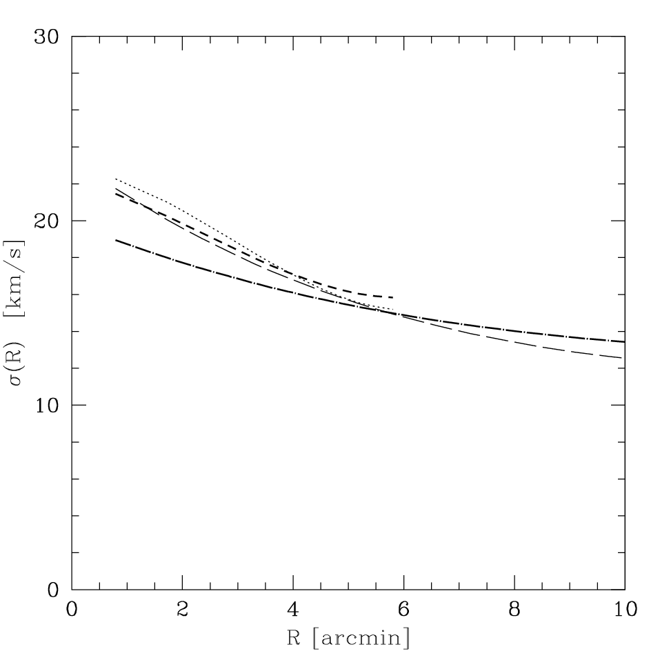
vL00 divide their proper motion observations into 4 classes based on the errors in the proper motion determination which depend upon crowding and plate quality. We only use stars with well measured proper motions (class 0) since their errors appear to be relatively well behaved (see Fig. 11 of vL00). Class 1 stars are slightly disturbed by a neighbour and are localized in the central part of the cluster. A comparision of the velocity dispersion curves in Figure 3 indicates that class 1 stars have a higher tangential velocity that class 0 stars in the central of the cluster.
3.3.1 Pre-processing of the Data
Following vL00, the centre of the cluster was taken to be 20169065, -4747855. To start off, we assume that the distance of the cluster is 5.5 kpc. We project the absolute celestial coordinates and into Cartesian coordinates (relative to the cluster centre) onto the plane of the sky perpendicular to the line-of-sight vector through the cluster centre (König, 1962):
| (8) |
and
| (9) |
where is a scaling factor ( to have and in radians and to have and in units of degrees), and are the cluster centre coordinates, and and .
We corrected the proper motion data for apparent rotation arising purely from projection effects using a canonical distance of 5.5 kpc and a systematic l.o.s velocity of km/s (vdV06). Any solid-body rotation cannot be determined from the differential proper motions due to the astrometric reduction process employed to measure the proper motions in the first place. However it can contribute significantly to the kinematics of the cluster. We correct for such a residual solid-body rotation with mas/yr/arcmin following vdV06.
3.3.2 Construction of Samples
vL00 calculate the membership probability of each star on the basis of its velocity and its projected distance. Choosing cluster members based merely on these membership probabilities is fraught with error, as they are correlated with radial completeness, mean radial distance and the limiting magnitude. Figure 4 demonstrates how the completeness and velocity dispersion of the sample correlates with the assigned membership probability, thereby affecting the mass estimate. Samples with higher cut-off membership probabilities are not only radially incomplete but also have lower velocity dispersion curves and hence lower estimated masses.

On the other hand, vdV06 select their sample by choosing those stars whose proper motion errors were lower than mas/yr after a proper motion membership cutoff of at least 68 percent, obtaining a limited sample of 2295 stars.
For the purpose of kinematic studies it is crucial to determine cluster membership in a way that is independent of the star’s velocity. In the subsequent analysis, we will therefore base cluster membership predominately on photometric properties.
In the trade-off between purity and size of photometrically selected samples, we consider two cases. Sample A: we consider only the horizontal branch stars in vL00 data, where field contamination is apparently negligible. Selecting horizontal branch stars in the ranges and , we get a total of 1053 stars.
Sample B: we correlate the Rey et al. (2004) published sample of cluster members based on photometry with the vL00 data (Sample B). The high precision BV photometry of Rey et al. (2004) data combined with the Ca and Stömgren by photometry (Rey et al., 2000), efficiently separates cluster stars from the typical disk field stars. To match the vL00 and Rey et al. (2004) data-sets, we first had to align them. We mapped the two data-sets using the IRAF CCMAP routine. We then cross-matched the two data-sets in a four vector space (RA, DEC, B and B-V). For the magnitude and colour, we gave a large leeway of 0.5 and 0.1 respectively. The size of the search window of the RA-DEC was (). We matched a total of 3321 stars.
However, this photometric approach leads to manifest outliers, stars that photometricaly look like Centauri members but whose velocity is far greater than the presumed escape velocity. Such stars will bias any mass estimates. Therefore, it is important that we also clean the sample kinematically of such outliers while introducing as little bias as possible. To do this, we calculate iteratively the velocity dispersion and excise stars outside , until all the stars are within the dynamical bounds. For Sample A, this clipping removes of the stars leading to 968 members. For Sample B, stars are removed by the clipping, bringing the numbers of stars in the sample to 3241.
Using the radial velocity data of Reijns et al. (2006), we can derive an independent rough estimate of the number of field stars in our sample. For the cleaned Sample B, out of the total of 1028 matched stars between the two samples, 22 stars were found to be field stars. The probability of the number of fields stars in the sample is . Given the additional data made available by the radial velocity data, we can do better.
Sample C: both Sample A and Sample B suffer from radial incompleteness, with Sample B extending partially upto R. We can extend the sample with the help of the radial velocity data of 1589 cluster stars of Centauri published by Reijns et al. (2006). By using only stars of class 0, we have 1276 stars which are 100% kinematically-certified cluster members that extend from to . Removing the 1028 common stars and the 22 field stars of Sample B, we get a total of 3467 stars. After a 3-sigma clipping, we get 3384 stars (Sample C). Out of these 3335 stars are within 20’.
Following vdV06, we only use stars within for the ML estimators. The ML estimators are independent of the spatial completness of the sample. Possible field stars with high velocities may unnecessarily bias the ML estimator.
On the other hand, we use the complete Sample C for the PME so as not to bias the estimator at the outer edges of the cluster. In the PME, the estimated mass involves an averaging process over the entire length of the cluster and hence completness is important. However, any sample so constructed is still incomplete near the center of the cluster due to crowding effects. This issue was raised in Subsection 2.1 and will be partially addressed in Subsection 3.3.4.
Therefore in the final analysis we will only use Sample C stars with the ML estimators for the cluster mass estimates. Sample A stars are limited in number and have large errors associated with their proper motion. Similarly Sample C is superior to Sample B in that it has a slightly higher number of stars and fewer contaminated field-stars. Nevertheless, we will also implement the PME with Sample A and Sample C in Subsection 4.1 to get a feel as to how the estimator fares.
3.3.3 Velocity Dispersion
The projected radial and tangential velocity dispersion profiles for Sample C as a function of projected distance R is shown in Figure 2 using radial bins from vL00 (Table 6). For comparison, we show the projected radial and tangential velocity dispersion profile of the sample of 2295 stars used by vdV06 in Figure 5. In general, the velocity dispersions are very similar, even though the evidence for a tangential anisotropy in the outer parts is weaker in our (cleaner) Sample C. It must also be noted that the velocity dispersions at larger radii () are highly uncertain, due to the small number of stars in these radial bins.

3.3.4 Radial Profile
Implicit in the methodology of Section 2 is the assumptions that the stars with measured kinematics fairly trace the overall population that yields the density profile, or . However, crowding effects and poorer colour information at the centre of the cluster leads to a bias in the radial sampling of stars with proper motions. This affects our sample. For example, we find that fainter sub-samples of Sample C lie at larger radii; proper motion estimates for them are precluded by crowding at smaller radii.
To model the surface number density, we fit a King density profile to the surface density data (see Figure 2) published by Ferraro et al. (2006). The probability distribution, , () for stars in each radial bin is shown in Figure 6. We can see that Sample C must be radially incomplete both near the centre of the cluster and at larger radii. Such radially incomplete samples will affect the mass estimates from those estimators which use an averaging process like the PME.
For the PME, we can attempt to recover back the original density profile by repeatedly sampling the same stars. While this is possible at the centre of the cluster because of the large number of available stars in the sample in those radial bins, it is difficult at the edge of the cluster () where the number of stars found in Sample C is much less than the numbers derived from the surface density profile. While repeatedly sampling the same stars may recover in some way the density profile, it may skew the velocity distribution. For example, repeatedly sampling stars that intrinsically belong to the outer edges of the cluster but which are projected towards the centre of the cluster, may alter the projected velocity distribution at the centre of the cluster. Similarly the limited number of stars at the outer ends of the cluster can bias the higher velocity moments.

4 Mass Estimators for Centauri
In this section, we connect the methodology of Section 2 with the data sets of Section 3 to estimate the mass of Centauri. We start by applying the PME (Eq. 2), then move on to ML-models (Section 2.2) based on a King model and the Jeans equation.
4.1 Projected Mass Estimator
To apply the PME, we first have to adjust our Sample A and C to fairly trace the overall population as a function of radius (Figure 6). We do so by Monte-Carlo drawing members from Sample C so that their radial distribution matches the profile of Ferraro et al. 2006 (solid line Figure 6).

The resulting PMEs are depicted in Figure 7, with the 1- error bars calculated from bootstrapping. For bright magnitude limits, we have only high precision measurements, but few stars. The larger error bars demonstrate the lack of information due to the limited amount of tracers of the system.
At magnitude 16, the PME estimates the mass of the cluster for Sample C as , while Sample A predicts for the same magnitude.
Note, that the inclusion of the error terms leads to an estimator that is virtually independent of (i.e., signal-to-noise). The high mass estimate reveals that the sample is radially incomplete especially at the center of the cluster.
4.2 Simple Maximum Likelihood Models
We now proceed to combine the dynamical models directly with ML estimates for the Centauri data to constrain the mass of the cluster.
We start off with the classic King model (King, 1966) framework for this task, then use the spherical isotropic Jeans equation to predict the velocity dispersion curve; in the subsequent section we generalise this to anisotropic, axisymmetric Jeans models
4.2.1 King Models
In Figure 8, a King profile (King 1962) is fit to number density profile of Centauri (Ferraro et al. 2006) characterized by the core radius, , and the concentration, . We found and . Note that these values are different from those originally derived from Ferraro et al. (2006) as the values they derived correspond to a dynamic King model (Sigurdsson & Phinney 1995). Given the King profile, we can derive a velocity dispersion profile using the technique outlined in King (1966) or by integrating the Jeans equaton. Even though the surface density profile provides a relatively good fit, the model cannot reproduce the projected velocity dispersion. If we nonetheless use this King model and the likelihoods equation 6, we obtain mass estimates for different magnitude limits (shown in the right panel of Figure 8).
For example at , the mass estimate is , with the error derived using likelihood methods. To compare the various models with each other, we can define a measure of the scatter as the range of mass estimates at various limiting magnitudes divided by the mass estimate at . The scatter for the King model amounts to .


4.2.2 Spherical Isotropic Jeans Model
The isotropic Jeans equation for a spherical system (neglecting rotation) is:
| (10) |
where is the radial velocity dispersion, is the observable number density distribution, and is the potential generated by the matter distribution at the considered point.
We use the three dimensional number density distribution by Merritt et al. (1997) derived using non-parametric analysis (left panel of Figure 9). We assume that mass follows light, and that the density profile also defines the potential of the cluster. The velocity dispersion is then predicted by Jeans equation. This is shown in the central panel of Figure 9. The velocity dispersion curve is then used to predict the mass of the cluster using the MLM.


As in Section 4.2.1, the error-bars with bright are large due to lack of information in the limited number of tracers. At magnitude 16, the MLM with the Jeans model estimates the mass of the cluster as for Sample C stars. The scatter of this model as defined earlier in Section 4.2.1 is .
The resulting MLM mass estimates of the cluster for the King model and the spherical isotropic Jeans model are consistent with each other.
The scatter in the results is indicative of the poor fit of the spherical models to the complex nature of Centauri. The results of the MLM are also not consistent with the results of the PME and those of vdV06. This indicates that we are poorly modelling the cluster, failing to take into account the apparent rotation and the flattening of the cluster. Hence we now turn to more sophisticated models, namely the anisotropic axisymmetric Jeans model.
4.3 ML Estimates based on anisotropic axisymmetric Jeans Models
Anisotropic axisymmetric Jeans modelling (e.g. Cappellari 2008) is one way to model Centauri without the restrictive approximations of isotropy and spherical symmetry. Ample evidence exists that neither approximation holds: Centauri’s velocity distribution is anisotropic (Anderson 2002; Anderson & van der Marel 2010; vL00; vdV06). Geyer, Hopp & Nelles (1983) have showed that Centauri is one of the most flattened globular clusters in the Galaxy.
In the case of Cappellari (2008), the semi-isotropic axisymmetric Jeans formalism is generalised to include anisotropy on the basis of two assumptions: a constant mass-to-light ratio and a constant velocity anisotropy parameter . Given a detailed description of the surface brightness in the form of a multi-Gaussian expansion (MGE), the model can predict the shape of the second velocity moments () on the basis of two free parameters and the inclination of the cluster. We calculate the relevant formulae for the second velocity moments for the two components of the proper motion in Appendix B. For the first velocity moment (), additional assumptions are required. Obtaining the rotation of the cluster from this formalism involves the need of separating the second moments into random and streaming rotation around the symmetry axis by the introduction of an additional parameter (and hence assumptions) for the first order equation (in terms of ; see Equation 35 of Cappellari 2008), analogous to the Satoh (1980) approach. The advantage of using a multi-Gaussian expansion (MGE) is that it allows us to set the rotation () and the anisotropy () individually for each Gaussian component.
Such modelling is based on the two-dimensional surface density distribution of the stars, which has not been published as such. However vdV06 have derived a multi-Gaussian expansion (MGE) of the one-dimensional V-band surface brightness profile of Meylan (1987) using 8 Gaussians. They converted this into a two-dimensional luminosity distribution by assigning a projected flattening to each Gaussian using the data of Geyer, Hopp & Nelles (1983). Unfortunately, these eight flattened Gaussians do not result in the elliptic profile of Geyer, Hopp & Nelles (1983), which increases upto and then falls again towards larger distances (Figure 10, left panel). We rederived a multi-Gaussian expansion to the number density profile of Ferraro et al. (2006) once more using 8 Gaussians. Using a Levenberg-Marquardt algorithm, we optimised the flattening coefficients to reproduce the Geyer, Hopp & Nelles (1983) data as shown in Figure 10 (left panel).
| k | ||||
|---|---|---|---|---|
| 1 | 1290.195 | 0.47557 | 1.000000 | 0.0 |
| 2 | 4662.587 | 1.931431 | 0.9991714 | 0.0 |
| 3 | 2637.784 | 2.513385 | 0.7799464 | 0.4 |
| 4 | 759.8591 | 3.536726 | 0.724126 | 1.1 |
| 5 | 976.0853 | 5.403728 | 0.8556435 | 0.6 |
| 6 | 195.4156 | 8.983056 | 0.9392021 | 0.0 |
| 7 | 38.40327 | 13.93625 | 0.9555874 | 0.0 |
| 8 | 8.387379 | 20.98209 | 1.0000000 | 0.0 |


We follow vdV06 in using an isophotal position angle of , and align our coordinates axes (,) with the observed isophotal major and minor axis of Cen.
An important parameter in an axisymmetric model is the inclination of the cluster () which relates intrinsic and projected flattening. This can only be constrained by including the line-of-sight velocity data, which vdV06 have done. They arrived at a joint constraint for the inclination and the dynamical distance under the assumption of axisymmetry: kpc. Using their dynamical models (an axisymmetric implementation of Schwarzschild’s orbit superposition method), they constrain further the inclination at and the dynamical distance. Even though Krajnović et al. (2005) and Cappellari (2008) have pointed out a degeneracy between the inclination and the anisotropy of the cluster, we adopt the inclination value from vdV06. The combination of the distance and the inclination we have adopted is consistent with the above relation.
To fix (see Equation 35 of Cappellari 2008) required for the parametrisation of the random and ordered streaming motion around the cluster, we must compare the model projected differential rotation with those derived from the cluster data. We use the polar aperture grid for the proper motions of vdV06. To derive the differential rotation of the cluster we use the non-parametric approach of Merritt et al. (1997) on the binned data, where we minimise the “penalised log likelihood” (see Equation 4 of Merritt et al. 1997) and used a ‘thin-plate smoothing spline’ routine found in the R-package ‘FIELDS’. We forced the velocities at large radii () to go down to zero, so that the main features at lower radii do not get swamped by the thin-plate spline routine. The differential rotation velocity contours are shown in the upper panel of Figure 11. Note that any solid-body rotation of a cluster cannot be determined from the differential proper motions.
Given the inclination (), we can proceed to derive for each Gaussian component by comparing the rotation curves with those predicted by the model. The resulting values of are given in Table 1. It must be noted that the peaks of rotation do not lie along the isophotal major axis along the y direction. If Centauri were exactly axisymmetric, the kinematic minor axis would coincide with the isophotal minor axis. However, Figure 11 shows that this is only approximately true. A similar feature was noted by Merritt et al. (1997) for Centauri while deriving the rotation curves from the line-of-sight velocities.

The anisotropic Jeans model allows us to set the anisotropy of each Gaussian component (). However we follow the practical approach of setting a global anisotropy parameter (see Section 4.3.1), which we can derive from the proper motion data after fixing the rotation of the cluster. Similar to Equation 7, we can construct a maximum likelihood estimator. The probability for measuring a given individual proper motion and , given the parameters and are:
| (11) | |||||
with a corresponding equation for . To obtain the global anisotropy parameter , we marginalise over the mass . We then maximise the likelihood for our Sample C, varying only the parameter b. Following standard practice, we can parameterise this anisotropy with the variable , where is the line-of-sight direction. Using Sample C, if the inclination of the cluster is fixed at , we find indicating that overall the cluster is close to isotropy.
We also calculate the 2-dimensional velocity dispersion profile of Sample C along the major and minor axis using a thin-plate spline (see Equation 11 of Merritt et al. 1997) and compare them with the model velocity dispersion profiles (see Equations 20 and 15). The results are shown in Figure 12. The dispersions were calculated using the polar apertures given in Table 3 of vdV06 and the standard techniques outlined in Appendix A and then fed to the thin-spline routine. Note that the elongation of the iso-dispersion velocity contours along the minor axis is not consistent with the assumptions of axisymmetry.

With an estimate of the global anisotropy parameter , we can now obtain the mass of the cluster using the MLM (Equation 6) in combination with Equation 11 for each component of the proper motion using Sample C. For each star in Sample C, we calculate the first and the second velocity moments for both the components of the proper motion (see Equations 22, 21, 20 and 15). The final mass estimate using our own derived values of flattening in Table 1, is shown in Figure 10. The good fit of the model is reflected in the low scatter in the mass estimates: the scatter of this model as defined in 4.2.1 is . The mass of the cluster using the anisotropic Jeans model is at the limiting magnitude .
4.3.1 Effects of Anisotropy, Inclination, Rotation and Flattening on the Mass Estimate
Within such a modelling context, it would be instructive to separate the effects due to inclination, rotation, anisotropy and flattening of the cluster.
While the value of the inclination of the cluster is consistent with the distance (5.5 kpc) we have adopted and the relation kpc, we do have a range of acceptable inclination degrees. However, with the assumptions of axisymmetry, the observed projected flattening of the cluster sets further constraints on the inclination of the cluster. From Eq. 14 of Cappellari (2008), the inclination is constrained by the flattening: . The fourth Gaussian of the MGE in Table 1 sets the lower limit of the inclination at . At , the mass inferred from Sample C is . At the lower end , the mass is , while at the higher end of , the mass is . Hence, the inclination of the cluster affects the mass estimate upto .
By neglecting the cluster rotation in the model, the mass inferred based on Sample C is ; if we include rotation, we get . Hence accounting for rotation affects the mass estimate for the cluster by only .
To isolate the effect due to anisotropy, we calculate the ‘best’ mass of the cluster for and . We get the same mass estimate in both cases. Hence we conclude that in such a modelling environment, the anisotropy of the cluster does not contribute much to the mass of the cluster. This is because the observed anisotropy is very small.
Accounting for the flattening of the cluster, however, is important. This is already apparent from the fact that the masses inferred via the flattened models are lower than our earlier estimates based on spherical models. To explore this further, we define for each Gaussian component a projected eccentricity . We then study how the estimate of the mass of the cluster varies as a function of the flattening parameter of the model in terms of the relative projected eccentricity , where corresponds to no flattening, while would correspond to the full flattening derived in Table 1. This results in a difference of nearly in the mass estimates as shown in Figure 13, which indicates the importance of properly determining the fattening of the cluster to determine its mass. Including also the effects of rotation along with the flattening profile of Table 1 further brings the mass to which is consistent with the results of vdV06.
At the dynamical distance of 4.8 kpc adopted by vdV06, this corresponds to a mass estimate of

4.4 Discussion of Centauri Mass Estimates
Our analysis presented here has made it clear that the major discrepancy in the estimated masses of Centauri arises primarily due to the choice of the modelling process. By taking into account both the flattening of the cluster and its inclination using axisymmetric models, and to a lesser extent by accounting for the rotation, we can derive consistently a mass estimate that has only error for a given distance.
However, even in our most complex modelling scenario, which included both anisotropy and axisymmetry, we had to draw on vdV06 to get a cluster inclination. Yet at the same time, we observed significant deviations in the 2-d velocity dispersion map. Our modelling has also shown that compared to the flattening, the inclination, anisotropy and the rotation, have less impact on the mass estimates. More accurate constraints must be put on the flattening of the cluster through more accurate two dimensional surface density profiles. Further, Centauri with its complex formation history is an ideal candidate for more sophisticated Schwarzschild modelling as attempted by vdV06. A perhaps more immediate step would be to incorporate radial velocity data in the MLM approach established here.
Irrespective of the modelling context, the largest uncertainty in our mass estimates based on proper motion data, arises from the adopted cluster distance, which scales the estimated mass as . In this paper, we have assume a distance of 5.5 kpc derived from RR Lyrae stars (Del Principe et al., 2006), with random and systematic distance errors of only each. This estimate is consistent with the estimate of the eclipsing binary OGLEGC 17 (Thompson et al., 2001), but substantially different from the dynamical distance of 4.8 kpc estimated by vdV06. Reliable dynamical distances depend on a host of factors - but crucially on a proper estimation of the velocity dispersions, which in turn is dependent on the proper selection of the sample. The estimate of vdV06 which is lower than that of Del Principe et al. (2006), could have come about if there is an over-estimation of the proper motion dispersion due to unrecognized interlopers or an under-estimation of the line-of-sight velocity dispersion. Intrinsic to these dispersion estimates is also a proper correction for perspective rotation (which is distance dependent) and solid-body rotation. Bono et al. (2008) report a systematic offset between reported absolute photometric distances and dynamical distances in the clusters Centauri and 47 Tuc, with dynamical distance estimates being lower. Therefore, relying on the precise and completely independent distance estimate from Del Principe et al. (2006) appears preferable. The distance errors translates into a error in the mass estimate.
As this paper is geared as a proof-of-concept paper of what is possible with proper motion data, we have steered away from directly using the line-of-sight velocity data. However, tackling the issues mentioned above warrants the use of the same. In such cases however, more sophisticated modelling schemes than what we have considered in this paper would be required to determine the dynamical distance of the cluster, which we postpone to a later paper.
5 Conclusions
In this paper, we implement two independent methods to determine the mass of a cluster from the proper motion data. Both the Projected Mass Estimator (PME) and the Maximum Likelihood modelling (MLM) provide unbiased and robust estimates of the mass of the cluster. However the use of the PME is limited due to a number of practical difficulties in sampling the cluster. For the MLM, we use an analytic King model, a spherical isotropic Jeans equation model and an axisymmetric, anisotropic Jeans equation model.
We apply these approaches to the extensive ground-based proper-motion data-set of Centauri by vL00. Using the high precision photometry of Rey et al. (2004), we construct a kinematically unbiased member samples, that should have less contamination than the samples used in previous analyses.
Among the three models used in the MLM context, the anisotropic axisymmetric Jeans equation with some rotation is by far the best model accounting for the photometric and kinematic data of Centauri, though there exists compelling evidence of deviations away from axisymmetry. Neglecting the flattening and inclination of the cluster by using spherical models overestimates the mass of the cluster by . This accounts also for the large spread in reported masses of Centauri.
The mass of the cluster is . The largest uncertainty in the absolute mass estimate is the distance to Centauri which enters as the third power. With a distance error of this amounts to a mass error of .
While our results are mostly consistent with those of vdV06, the difference arises due to our adoption of the new RR lyrae distance estimates and due to our more accurate reconstruction of the flattening and the shape of the MGE parametrization leading to an increase in the mass estimate by .
This estimate has a statistical error, but uncertainty arising from the distance errors.
The authors thank Glenn van de Ven for helpful comments on the manuscript. The authors also thank the referee for her patience and for helpful advice.
References
- Anderson (2002) Anderson J., 2002, in ASP Conf. Ser. 265: Omega Centauri, A Unique Window into Astrophysics, Main-Sequence Observations with HST. pp 87–+
- Anderson & van der Marel (2010) Anderson J., van der Marel R.P., 2009, ApJ, 710, 1032
- Bahcall & Tremaine (1981) Bahcall J., Tremaine S., 1981, ApJ, 244, 805
- Bellini et al. (2009) Bellini A., Piotto G., Bedin L.R., Anderson J., Platais I., Momany Y., Moretti A., Milone A.P., Ortolani S., 2009, A&A, 493, 959
- Binney, Davies & Illingworth (1990) Binney J. J., Davies R. L., Illingworth G. D., 1990, ApJ, 361, 78
- Bono et al. (2008) Bono G., Stetson P. B., Sanna N., Piersimoni A., Freyhammer L. M., Bouzid Y., Buonanno R., Calamida A., Caputo F., Corsi C. E., Di Cecco A., Dall’Ora M., Ferraro I., Iannicola G., Monelli M., Nonino M., Pulone L., Sterken C., Storm J., Tuvikene T., Walker A. R., 2008, ApJ, 686, 87
- Cappellari (2008) Cappellari M., 2008, MNRAS, 390, 71
- Del Principe et al. (2006) Del Principe M., Piersimoni A. M., Storm J., Caputo F., Bono, G., Stetson P. B., Castellani M., Buonanno R., Calamida A., Corsi C. E., Dall’Ora M., Ferraro I., Freyhammer L. M., Iannicola G., Monelli M., Nonino M., Pulone L., Ripepi V., ApJ, 2006, 652, 362
- Efstathiou, Ellis & Peterson (1988) Efstathiou G., Ellis R.S., Peterson B.A., 1988, MNRAS, 232, 431
- Emsellem, Monnet & Bacon (1994) Emsellem E., Monnet G., Bacon R., 1994, A&A, 285, 723
- Evans & de Zeeuw (1994) Evans N. W., de Zeeuw P. T., 1994, MNRAS, 271, 202
- Ferraro et al. (2006) Ferraro F. R., Sollima A., Rood R. T., Orgilla L., Pancino E., Bellazzini M., 2006, ApJ, 638, 433
- Genzel et al. (2000) Genzel R., Pichon C., Eckart A., Gerhard O.E., Ott T., 2000, 317, 348
- Geyer, Hopp & Nelles (1983) Geyer E. H., Hopp U., Nelles B., 1983, A&A, 125, 359
- Gnedin et al. (2002) Gnedin O. Y., Zhao H., Pringle J. E., Fall S. M.; Livio M.; Meylan ., 2002, ApJ, 568, 23
- Heisler, Tremaine & Bahcall (1985) Heisler J., Tremaine S., Bahcall J. N., 1985, ApJ, 298, 8
- Herbst et al. (2004) Herbst T. M., Ragazzoni R., Eckart A., Weigelt G., 2004, SPIE, 1042
- Hilker & Richtler (2000) Hilker M., Richtler T., 2000, A&A, 362, 895
- Hughes & Wallerstein (2000) Hughes J., Wallerstein G., 2000, AJ, 119, 1225
- King (1962) King I. R., 1962, AJ, 67, 471
- King (1966) King I. R., 1966, AJ, 71, 64
- König (1962) König A., 1962, in Hiltner W.A., ed, Astronomical Techniques, University of Chicago Press, p.471
- Krajnović et al. (2005) Krajnović D., Cappellari M., Emsellem E., McDermid R. M., de Zeeuw P. T., 2005, MNRAS, 357, 1113
- Kuijken & Dubinski (1994) Kuijken K., Dubinski J., 1994, MNRAS, 269, 13
- Lampton, Margon & Bowyer (1976) Lampton M., Margon B., Bowyer S., 1976, ApJ, 208, 177
- Leonard & Merritt (1989) Leonard P. J. T., Merritt D., 1989, ApJ, 339, 195
- Longmore (1992) Longmore A. J., 1992, in IAU Colloq. 139, 21
- Mandushev et al. (1991) Mandushev G., Staneva A., & Spasova N., 1991, A&A, 252, 94
- Mayor et al. (1997) Mayor M., et al., 1997, AJ, 114, 1087
- McNamara, Harrison & Anderson (2003) McNamara B.J., Harrison T.E., Anderson J., 2003, ApJ, 595, 187
- Merritt et al. (1997) Merritt D., Meylan G., Mayor M., 1997, AJ, 114, 1074
- Meylan (1987) Meylan G., 1987, A&A, 184, 144
- Miocchi (2010) Miocchi P., 2010, A&A, 514, 52
- Mizutani, Chiba & Sakamoto (2003) Mizutani A., Chiba M., Sakamoto T., 589, 89
- Page (1952) Page T., 1952, ApJ, 116, 63
- Prada (2003) Prada F., Vitvitska M., Klypin A., Holtzman J.A., Schlegel D.J., Grebel E.K., Rix H.-W., Brinkmann J., McKay T.A., Csabai I., 2003, ApJ, 598, 260
- Reijns et al. (2006) Reijns R.A., Seitzer P., Arnold R., Freeman K. C., T. Ingerson, van den Bosch R.C.E., van de Ven G., de Zeeuw P. T., 2006, A&A, 119, 1824
- Rey et al. (2000) Rey S.-C., Lee Y.-W., Joo J.-M., Walker A., Baird S., 2000, AJ, 119, 1824
- Rey et al. (2004) Rey S.-C., Lee Y.-W., Ree C.H., Joo J.-M., Sohn, Y.-J., Walker A.R., 2004, AJ, 127, 958
- Richer et al. (1991) Richer H.B., Fahlman G. G., Buonanno R., Fusi Pecci F., Searle L., Thompson I. B., 1991, ApJ, 381, 147
- Schödel, Merritt & Eckart (2009) Schödel R, Merritt D., Eckart A., 2009, A&A, 502, 91
- Suntzeff & Kraft (1996) Suntzeff N., Kraft R., 1996, AJ, 111, 1913
- Thompson et al. (2001) Thompson I. B., Kaluzny J., Pych W., Burley G., Krzeminski W., Paczynski B., Persson S. E., Preston, 2001, AJ, 121, 3089
- Trager, King & Djorgovski (1995) Trager S.C., King I. R., Djorgovski S., 1995, AJ, 109, 218
- van de Ven et al. (2006) van de Ven G., van den Bosch R.C.E., Verolme E.K., de Zeeuw P.T., 2006, A&A, 445, 513
- van der Marel, Binney & Davies (1990) van der Marel R. P., Binney J., Davies R. L., 1990, MNRAS, 245, 582
- van Leeuwen et al. (2000) van Leeuwen F., Le Poole R. S., Reijns R. A., Freeman K. C., de Zeeuw P. T., 2000, A&A, 360, 472
- White & Shawl (2000) White R. E., Shawl S. J., 1987, ApJ, 317, 246
- Wolf et al. (2010) Wolf Joe, Martinez Gregory D., Bullock James S., Kaplinghat Manoj, Geha Marla, Munoz Ricardo R., Simon Joshua D., Avedo Frank F., 2010, MNRAS, 406, 1220
- Wojtak et al. (2007) Wojtak R., Lokas E. L., Mamon G.A., Gottlöber S., Prada F., Moles M., 2007, A&A, 446, 437
Appendix A Velocity Dispersion
The projected velocity dispersion of the cluster is needed for the kinematic removal of outliers, and can be calculated in the context of a maximum-likelihood analysis (vdV06). For a given cluster member star with velocity at a given projected distance , the probability that the cluster has a dispersion is given by
| (12) |
where is the probability of measuring the velocity as defined in Equation 4 and is the probability of a star in the cluster to have a certain proper motion velocity given a velocity distribution parameterized by the velocity dispersion .
The projected velocity dispersion is then derived by maximising the likelihood function for a given number of stars drawn from a concentric ring centred around a projected distance :
| (13) |
with the uncertainty resulting from . Usually, Gaussians are a good low-order approximation for the velocity distribution , thus simplifying the process.
We can also modify the distribution function to account for the probability of the star to belong to the cluster (first introduced by Prada 2003; Wojtak et al. 2007):
| (14) |
where is the probability of the star to belong to the cluster, is the regular Gaussian distribution and is the maximum projected velocity in the particular annular ring where the dispersion is being calculated.
Appendix B Anisotropic Jeans Equation
Following the formalism of Cappellari (2008), we can calculate the second moments and the mean velocity along the two perpendicular axes projected on the plane of the sky. Cappellari (2008) have already indicated that the projected proper motion dispersion can be written via single quadratures. Similar to equation 28 of Cappellari (2008), we can derive the analogue expressions for the proper motions using the formulas in Appendix A of Evans & de Zeeuw (1994). The component of the velocity dispersion is:
| (15) | |||||
where we retain the definitions of , , , and . For the sake of completeness we repeat these definitions once again.
| (16) |
| (17) |
| (18) |
| (19) |
Similarly, the component of the velocity dispersion is:
| (20) | |||||
We can also obtain the proper motion first velocity moments of the whole MGE model similar to equation 39 of Cappellari (2008). The MGE model uses an anisotropic analogue of Satoh (1980) approach, as seen in equation 37 of Cappellari (2008), where fixes the rotation for each Gaussian component.
| (21) | |||||
| (22) | |||||
The velocity dispersion can then be calculated as:
| (23) | |||
| (24) |