The even-odd effect in short antiferromagnetic Heisenberg chains
Abstract
Motivated by recent experiments on chemically synthesized magnetic molecular chains we investigate the lowest lying energy band of short spin- antiferromagnetic Heisenberg chains focusing on effects of open boundaries. By numerical diagonalization we find that the Landé pattern in the energy levels, i.e. for total spin , known from e.g. ring-shaped nanomagnets, can be recovered in odd-membered chains while strong deviations are found for the lowest excitations in chains with an even number of sites. This particular even-odd effect in the short Heisenberg chains cannot be explained by simple effective Hamiltonians and symmetry arguments. We go beyond these approaches, taking into account quantum fluctuations by means of a path integral description and the valence bond basis, but the resulting quantum edge-spin picture which is known to work well for long chains does not agree with the numerical results for short chains and cannot explain the even-odd effect. Instead, by analyzing also the classical chain model, we show that spatial fluctuations dominate the physical behavior in short chains, with length , for any spin . Such short chains are found to display a unique behavior, which is not related to the thermodynamic limit and cannot be described well by theories developed for this regime.
pacs
75.50.Xx, 75.10.JmI Introduction
The antiferromagnetic Heisenberg model is the appropriate starting point to understand magnetism in a large variety of different materials where strong electron correlations are important. Within its context the quantum nature of magnetism reveals itself, leading to a vast array of fascinating phenomena. Accordingly this model has been the topic of numerous experimental and theoretical works in different combinations of magnetic lattices and spin magnitudes. Indeed, many interesting theoretical concepts have been developed specifically for the antiferromagnetic Heisenberg model in the thermodynamic limit,[1, 2, 3] including spin waves, effective Hamiltonians, quantum field theories, and hydrodynamic methods. However, as will be shown in this paper most of these methods fail when describing finite (but possibly large) clusters of spins, which show a unique behavior that strongly depends on the boundary conditions and topology and therefore form a separate class of magnetic materials.
The properties of the antiferromagnetic Heisenberg model on small clusters such as dimers, trimers and tetramers, which are relatively simple to understand, were mainly of relevance to chemists, as the Heisenberg exchange describes magnetic interactions between metal ions in polynuclear metal complexes very well,[4] and also allowed the investigation of the origin of the fundamental magnetic interactions.[5] However, the advances in the synthesis of metal complexes during the last fifteen years have produced nanosized magnetic molecules with up to a few dozens of magnetic metal ions interacting with each other via Heisenberg exchange, creating the new class of molecular nanomagnets.[6, 7] Molecular nanomagnets belong to the mesoscopic regime, and their magnetism can be considerably more complex than in few-membered metal clusters and possess a quantum many-body character, yet they may not contain enough spin centers to be appropriately described by the methods and techniques developed for extended systems. Apart from synthetic chemistry, artificial engineering of quantum spin clusters has also emerged in recent years.[8, 9, 10] Here clusters of magnetic ions have been fabricated directly on insulating surfaces, and their magnetic properties were measured with scanning tunneling microscopy.
Nanosized spin clusters are ideal to study basic questions of quantum mechanics in mesoscopic systems, such as the efficiency of different metal centers or topologies towards a desired magnetic property, or the transition from the quantum to the classical regime for larger ion spins.[11, 5] They also provide an ideal testing ground for the validity of different theoretical models. In this paper we consider the antiferromagnetic Heisenberg model with a small number of spins of magnitude placed along a chain of length with open ends,
| (1) |
where denotes a spin- operator on site and for antiferromagnetic interactions. We will show that despite the apparent simplicity of the model the detailed aspects of the spectrum are highly non-trivial.
The model for an infinite chain or one-dimensional antiferromagnetic Heisenberg chain (AFHC) has attracted enormous interest, especially after Haldane’s conjecture of a fundamental difference between integer and half-integer spin chains, which is by now well established.[12, 13, 14] Finite but long chains have also received significant attention, but mainly for connecting numerical results to the thermodynamic limit via scaling [15] or for understanding boundary,[16] impurity,[17] and doping effects.[18] On the other hand, very little has been done for short chains with , in which the Haldane gap is always smaller than the finite-size excitation energy, and the difference between integer and half-integer spins is thus expected to become irrelevant.
Short AFHCs have recently become accessible experimentally, e.g., through the synthesis of molecular Cr3+ () modified wheels and horseshoes.[19, 20, 21, 22, 23, 24, 25] Two Fe3+ containing ring molecules were also studied, which magnetically represent chains of lengths and .[26, 27] Magnetic and inelastic neutron scattering measurements on the Cr6 and Cr7 horseshoes (, and ) have provided a detailed view on the magnetic excitation spectrum of these clusters,[19, 20] and pointed to systematic differences between chains with even and odd number of spins. The expected even-odd effects were found, such as total spin and in the ground state for even and odd respectively, which can obviously be associated to the interplay of the open boundary conditions and the symmetry requirements. However, a more subtle but striking difference in the energy spectrum has also been noted in addition, which we here refer to as the even-odd effect.
This even-odd effect manifests itself in the lowest energy band as a function of total spin , which depending on the context is known as the tower of states, quasi-degenerate joint states, or the band.[28, 29, 30, 31] In this band the energies are expected to increase as , and for bipartite spin systems it is generally possible to use a simplified model, the Hamiltonian, to describe it. The model has been very successfully applied to even-membered antiferromagnetic Heisenberg rings (odd-membered rings will not be considered in this work),[31] and experimentally confirmed in fine detail for the Cr8, CsFe8 and Fe18 molecular wheels.[32, 33, 34] Further examples are the Mn-[33] grid and the Fe30 Keplerate molecules.[35, 36, 37, 38, 39] For short chains with open ends, however, the approximation of the band appears to work very well for odd chains, while for even chains it surprisingly fails in the low energy sector.
We here explore alternative approaches to extract the essential physics of the AFHC model for short chains. In particular, we carefully reanalyze the model, and compare numerical diagonalization results for Eq. (1) with the predictions of field theoretical approaches, the classical AFHC, and parent valence-bond Hamiltonians. These approaches differ in their treatment of the quantum and spatial fluctuations and allow us to get insight into the roles played by them.
As main results we will demonstrate that the edge-spin picture, which has been firmly established for long chains for [40, 41, 42, 43] and higher ,[44, 15, 45] and was conjectured to stay robust up to very small ,[15, 45] is not consistent with our exact numerical data, justifying our distinction into short and long chains. Furthermore, for spins the even-odd effect has converged already closely to the classical behavior, yet quantum fluctuations are still noticeable. We finally conclude that short AFHCs posses simultaneously a classical and a quantum character, blurring the limit between classical and quantum behavior.
The paper is organized as follows: in Sec. II the even-odd effect is introduced, and the model is analyzed in Sec. III. Section IV deals with the predictions of the O(3) nonlinear -model, which originates in a path integral representation. Section V goes away from semiclassical descriptions to investigate quantum mechanical effects on the extreme quantum case. The classical limit of the AFHC is investigated in Sec. VI, and spin density and correlation effects in Sec. VII. The valence-bond model description of the AFHC is analyzed in Sec. VIII and finally, Sec. IX presents the conclusions. The Appendices that then follow include relevant information on various topics of the main text.
II The Even-Odd Effect

The different symmetry properties between even- and odd-membered AFHCs naturally generate differences in the magnetic properties, which show up in various quantities giving rise to various ”even-odd” effects. The most obvious difference is in the ground state, which has total spin for even and for odd chains due to the residual spin, as can be inferred from the classical antiferromagnetic spin configuration in the ground state, or the theorem of Lieb and Mattis.[46] Pronounced differences are also present for example in the spin density and spin correlation functions (see Sec. VII), which are however largely dictated by symmetry and boundary considerations.
The even-odd effect observed in this paper is related to pronounced deviations from an approximate energy dependence, and through this is associated to the model, or more generally the - and -band picture of the excitations in not too large bipartite spin clusters (the -band collectively denotes the next higher lying rotational bands).[7] In this section we define and characterize the even-odd effect. The model and the -band picture will be described and reanalyzed in more detail in the following section.
The Hamiltonian of Eq. (1) is SU(2) invariant and the eigenstates are organized as multiplets of degenerate states according to . We focus on the lowest spin multiplet in each sector, i.e., the band. Starting from the ground state, the energies of the lowest spin multiplets increase approximately as (consistent with the Lieb-Mattis ordering of energies [46]). They thus fall approximately on a straight line in an energy vs. plot, which is the band. The ground state spin will be denoted by , and that of the state with maximal spin or ferromagnetic state by . The region in the energy spectrum with small (large) values of will be called the antiferromagnetic (ferromagnetic) region. Energy values are always presented with respect to the ground-state energy. The eigenvalues and eigenstates of Eq. (1) have been calculated by full exact, subspace iteration and/or Lanczos diagonalization, with the Hamiltonian matrix represented in the product space or by irreducible tensor operators [4], and spatial symmetry was also used [47, 48] (see Appendix A for more details).
For illustration, Fig. 1 shows spectra of AFHCs with and for both and . While it is clearly possible to identify the band, there are systematic deviations. In particular, for the band is no longer well approximated by an dependence for small . In contrast, for the behavior is surprisingly well obeyed. Depending on the view point, the question hence arises why the band deviates from the behavior so strongly in the even chain, or why is it so well realized in the odd chain.
In order to characterize the differences between even and odd we consider the (normalized) slope of the band in the vs. representation as a function of ,
| (2) |
with , which is the discretized version of . The slope is normalized with the quantity , which is given for even and odd chains, and rings (for comparison), as
| even chain: | |||||
| odd chain: | |||||
| even ring: | (3) |
The normalization allows us to directly compare with the predictions of the model, for which (see Sec. III). It is noted that the difference of for the even ring and the chains is of order while that for the even and odd chain is of order , and that the slope emphasizes differences in the antiferromagnetic region.
Experimentally, the energies are directly connected to the low-temperature magnetization curve , and their differences can be extracted from it ( is the magnetic field). In a magnetic field the energies are modified as (assuming a gyromagnetic factor equal to 2), and at zero temperature is discontinuous with steps of height at fields . An energy dependence with an appropriate gap yields steps at regularly spaced fields , and deviations from the energy dependence or a constant slope are detected as deviations from this regular field pattern. If one extrapolates through the magnetization steps or measures the magnetization at elevated temperatures, the curve increases linearly with field (except at very low fields), and deviations from the behavior are observed as a field-dependent slope or non-constant susceptibility . For the classical case the slope can in fact rigorously be shown to be proportional to the inverse susceptibility (Sec. VI). The energy differences can also be measured directly by inelastic neutron scattering due to the selection rule , permitting a spectroscopic determination of the slope .
The slope is plotted for and for ranging from 1/2 to 7/2 or 3 in Fig. 2. For , which represents odd chains, varies weakly with (at least for ), and is close to 1. In contrast, there is a strong reduction of the slope for , the representative for even chains, for . In comparison to the maximal total spin the region of strong deviation is thus given by , and the disagreement with the spectrum does not alleviate with increasing , contrary to naive expectation. The deviation is pronounced for a wide range of values for short chains, but for long chains where it becomes very limited in range and is less important. These observations are a major result of this paper and establish the even-odd effect considered here.


The even-odd effect is most pronounced in the antiferromagnetic region and hence also the slopes
| (4) |
are considered, which characterize the antiferromagnetic and ferromagnetic parts of the band respectively [see Figs 1(a), (b)]. In Fig. 3 is plotted as function of for various . Since in Eq. (3) is slightly smaller for even than for odd chains, the scaling by mitigates the even-odd difference in as compared to the non-normalized slope. Nevertheless, the difference between even and odd chains is obvious. Interestingly, the difference between the even and odd grows with . This divergence suggests that the excitations on the band in the antiferromagnetic region have different physical origin for even and odd chains. For much larger the behavior known for long chains will be approached. The ferromagnetic slope can be calculated exactly from the lowest one-magnon energy as[14]
| (5) |
Hence, as is just the classical one-magnon energy for a particular wave vector, the even-odd effect is absent in the ferromagnetic regime. We note that using Eq. (5) one finds for . This is an important difference to even-membered rings, where due to translational invariance the eigenvalues and eigenfunctions of the lowest one-magnon state are equivalent to those of and hence for all ring sizes.[31] The absence of the even-odd effect in the ferromagnetic region is also seen in the spin density in the lowest one-magnon state, given by
| (6) |
There is no qualitative difference between even and odd here.

It is also of interest to consider the lowest energies in odd chains for , since the model (Sec. III) and the edge-spin picture (Sec. IV) predict distinctly different trends with for these states. The energies in this region can be represented by the normalized excitation energies
| (7) |
shown in Fig. 4 for the chain for to 5. The energies get smaller with increasing , , and the dependence on is essentially linear with a small curvature.
We conclude this section by discussing the different symmetry properties of even and odd chains. The mirror symmetry about a central site for odd chains can support a Néel-type antiferromagnetic configuration in the ground state [as indicated in Fig. 10(b), top picture]. Even-membered chains on the other hand are mirror symmetric about a link and cannot show any local magnetization in the ground state. In this case an alternating quantum dimerization is more suggestive if is not very large, where neighboring spins are more strongly correlated on odd links and less on even links. Another difference is that possible residual spin degrees of freedom at the edges, the so-called edge spins, first introduced in the context of valence bond ground states and long AFHCs,[49, 50, 40, 43] are effectively coupled ferromagnetically for odd and antiferromagnetically for even (Sec. IV.3). Notably, rings with periodic boundary conditions always possess mirror symmetry about a link and a site for both even and odd , so that there is no fundamental symmetry difference as in chains. For chains the symmetry properties of the lowest multiplets in each sector , which for represent the band, are summarized in Table 1,[48] in agreement with the findings for the chain in Ref. [51]. It is also noted that multiplets in a specific sector share the spin-flip parity of the corresponding state of the band, whenever this is a good quantum number.
| mirror | spin-flip | ||||
|---|---|---|---|---|---|
| parity | parity | ||||
| even | integer or half-integer | ||||
| odd | integer , | ||||
| odd | integer , | ||||
| odd | half-integer , | - | |||
| odd | half-integer , | - |
III The Model
For a number of bipartite molecular nanomagnets with antiferromagnetic Heisenberg interactions such as regular even wheels, modified even wheels, and grid molecules, the lowest lying spectrum was observed to consist of rotational bands or sets of states whose energies increase as , with appropriate gap and ”dispersion relation” , where is a suitable index or quantum number.[28, 29, 31] The lowest band ( band) and the set of higher-lying bands ( band) are distinguished according to a selection rule and the different nature of the excitations associated to them. This structure of the excitations is reminiscent to that shown in Fig. 1 for the AFHCs, and the energy dependence is indeed well obeyed for the odd chains, but as was demonstrated in the previous section pronounced deviations occur in the antiferromagnetic region for the even chains. In order to examine the even-odd effect the -band picture is therefore reanalyzed.
In the band picture the band is described by an effective Hamiltonian of two collective spins,[31]
| (8) |
where and are the total spin operators of the two sublattices and . The value of can be determined using symmetry or mean-field arguments,[52, 30, 31, 53] and is given for chains and rings in Eq. (3). The eigenvalues of are easily determined to be
| (9) |
where . For given values of and the energy spectrum consists of rotational bands. In the band and assume their maximal values, and the slope is calculated to . The next higher-lying states of , which involve the states where either or is reduced by one, are related to the band. However, they do not reproduce the energies of because the spatial fluctuations, which give rise to dispersion of these excitations, are not accounted for in the model [that is, is not obtained correctly].[31]
Based on the observation that the energies follow an dependence and that the calculated eigenvalues and matrix elements become quantitatively exact for large , the model has been called classical or semi-classical. However, this notion is misleading as retains a quantized spectrum. The basic underlying assumption of the model is in fact that the correlation length is infinite. The model could then be regarded as a symmetrized version of the bipartite Heisenberg Hamiltonian, and in fact it is part of the greater class of the symmetrized effective Hamiltonians which we introduce next.
With a unitary symmetry operator , a translation operator for example, the symmetrized effective Hamiltonians are constructed as follows: if a Hamiltonian remains unchanged after transformations with ,
| (10) |
for example if , then an effective Hamiltonian is formed by adding up all transformations of ,
| (11) |
This effective Hamiltonian commutes with , since . A common eigenbasis can thus be found where the eigenvalues of the unitary have magnitude 1, and one derives from Eq. (11)
| (12) |
since for any . If then perturbation theory is applied to a non-degenerate eigenstate using , is found to be exact in first order according to Eq. (12). This establishes also an upper bound for the ground-state energy of , in any spin sector if is SU(2) invariant, as the higher orders in perturbation theory will result in a negative contribution by the variational principle.
is obtained if is a sublattice permutation operator, and it therefore follows that is exact in first order for non-degenerate energy eigenstates or SU(2) multiplets, respectively, and the band in particular [see Figs 1(a), (b)]. For odd chains and even rings, it suffices to use a translation operator on one (the bigger) sublattice. is then the size of the sublattice, and . For even chains the two sublattices have to interchange.
At this point it may be surprising that odd chains can be described by the model, as the two collective spins and are necessarily of different size and therefore the problem becomes less symmetric. However, much more important is the fact that the collective spins obey the mirror symmetry for odd , which is not the case for even (where and are interchanged by this symmetry operation). For even chains on the other hand the model would be expected to work well, in contrast to our findings. In a study on the , chain it was argued that the - and -band states mix producing deviations in the energies, which is forbidden in rings due to translational symmetry, at least in first order.[22] The argument is obviously correct, but does not provide further insight, in particular on the even-odd effect.
Except for energies with in the even chains, Fig. 2 could suggest that the model works otherwise well for chains. However, the slopes which approximate the band in the ferromagnetic region in Fig. 2 are significantly larger than what is predicted by Eq. (3). This is not easily accounted for within the model. The upper bound given by for the energies in the band is hence not very tight for both even and odd chains [see Figs. 1(a) and (b)], giving room to convex deviations from a dependence, which in the case of the even chains indeed occur for .
It is also interesting to inspect the lowest energies in odd chains for and compare to those of . predicts a linear dependence on , i.e., up to a constant or for . A linear dependence is indeed observed in this spin sector as shown in Fig. 4, but the slopes are much lower than what is predicted by . This is attributed to the neglected spatial fluctuations or dispersion of the excitations, which generally lowers the minimal energy.
For even rings and other bipartite clusters it is well established that the model becomes more valid the smaller and/or the larger is.[31, 54] Regarding chains, a similar tendency should be expected, which is not observed; e.g. the even-odd effect persists for large as discussed in Sec. II. In contrast to rings the open boundaries in chains induce inhomogeneities, which are apparently not properly reflected in a model with infinite correlation length.
Taken together, the model appears appealing at first sight based on its energy dependencies, which are consistent with the energy spectrum in the AFHCs up to the even-odd effect displayed in Fig. 2, and because it is exact in first-order perturbation theory. However, the detailed analysis revealed its deficiencies, which appear to be connected to its neglect of spatial fluctuations or the assumed infinite correlation length.
IV Path integral representation: The O(3) nonlinear -model
The O(3) nonlinear -model (NLSM) has the potential to be suitable for short chains as it is based on the large spin, semiclassical limit, and can take inhomogeneous states into account. In general, boundaries lead to residual topological contributions in the effective action for both half-integer and integer spin chains,[55] a concept that goes beyond the physics the model is capable of describing. In the following we relate the concepts of the O(3) NLSM with the numerical findings for the spectra of the antiferromagnetic Heisenberg model on short chains. In the limit of vanishing spatial fluctuations we indeed identify rotational bands in the spectra. For long chains the topological boundary terms have been interpreted as remaining free spins at the edges of the chain (edge spins).[44, 43] We show that this interpretation is not supported by our numerical data and cannot explain the even-odd effect in the spectra of short AFHCs. On the contrary, we find that in short chains the alternating magnetization can no longer be separated from the uniform magnetization, as it is assumed in many theories.
IV.1 Derivation of the O(3) NLSM
The O(3) NLSM originates in an effective path integral representation of the AFHC in the low energy continuum limit[12, 13] (see also Appendix C). The Euclidean action of a single isolated spin with Hamiltonian is best expressed in terms of spin coherent states reading[2]
| (13) |
where . States are labeled by a three-dimensional unit vector defined by the eigenstate equation . The kinetic energy of the spin enters in the last term in Eq. (13), defined as
| (14) |
where is the region bounded by the closed curve on the unit sphere. The auxiliary variables and parametrize . The action is unambiguously defined provided that is an integer.[56] It should be pointed out that in deriving the action in Eq. (13) the assumption that is of order is used. However, there is no physical reason why the difference of two paths at adjacent time steps should be a small quantity.[57] Only for large the overlap of two spin coherent states becomes infinitely small [2], and therefore only in this limit the action in Eq. (13) becomes exact.
For finite chains of length the action , Eq. (13), generalizes to
| (15) |
where and is a product of single spin states on each lattice site. In order to derive an effective field theory some assumptions must be made which are justified in the low energy and large limit. Since it is expected that at least for short range order the chain exhibits sizable antiferromagnetic correlations, the local spin field is decomposed into a Néel field and a transverse canting field
| (16) |
where and is the lattice constant. The fields and are assumed to be slowly varying and chosen to fulfill and . Field contains the Fourier modes near and field those near , the ordering wave vector. Thus roughly represents the net magnetization, which is assumed to be small.
Then Eq. (16) is inserted in Eq. (15), is set and the continuum limit is taken. After some technical calculations (see Appendix C) the O(3) NLSM is generated:
| (17) |
with , and
| (18) |
In Eq. (17) the field has been integrated out giving . In order to understand the topological meaning of , for even Eq. (18) is rewritten as
| (19) | |||||
| (20) |
After evaluating the integral in Eq. (20) and taking into account an additional uncompensated Berry phase for odd,[55] one generally obtains
| (21) |
where is integer valued and simply counts the winding number of the field . For periodic boundary conditions and even, Eq. (21) reduces to , the so-called -term,[12, 13] where . depends only on the topology of the path.
In general, with respect to the derivation of Eq. (17) for open boundaries, when performing the continuum limit for open chains additional boundary terms in the action are expected to be found. In some cases these terms can simply be included by introducing an effective length. For alternating sums though, the cases of summing over an odd or even number of terms need to be distinguished. Higher order terms in the bulk action are found which are assumed to be small [see Eq. (C) in Appendix C].
The topological term in Eq. (17) is known to play a crucial role for the behavior in the thermodynamic limit. It enters the path integral with a factor , thus for integer spin it does not affect the partition function of the chain, while for half-integer chains yields an alternating factor . The renormalization group treatment of the action in Eq. (17) with the constraint leads to an increase of which is at first independent of at large energy scales. Without the topological term this leads to a strong coupling fixed point with a mass gap for integer spin chains, which has also been suggested from the calculation of the exact matrix.[58] However, with the topological term for the renormalization behavior is altered and becomes difficult to analyze at small energy scales, but it is known that half-integer spin chains are massless and belong to the universality class of the SU(2) Wess-Zumino-Witten model with topological coupling [59, 60, 61, 62] in agreement with the Lieb-Schultz-Mattis theorem [63] and the Bethe ansatz solution for the integrable spin- chain. This difference between integer and half-integer spin chains has become well-known in the literature.[12, 13] However, in the small chains that are considered in this work, the renormalization group flow is terminated by the finite length of the system at rather large energy scales, which exceed the mass gap, i.e., before makes a significant difference. Therefore, there is no need to distinguish between massive and massless theories in the following analysis.
IV.2 The Rotational Band in the O(3) NLSM
In order to connect with the model, spatial fluctuations in the action are initially ignored. The problem then reduces to a -dimensional one and the action of Eq. (17) taking into account Eq. (21) is given by
| (22) |
where , for even and for odd. For this yields the path integral of the -dimensional rigid rotator[64], with energy levels
| (23) |
where and each energy level is -fold degenerate.
The case can also be solved exactly, e.g., in the CP1 representation by introducing an independent gauge field.[65] This auxiliary field can be set to zero, and the Lagrangian becomes the rigid rotator Lagrangian again. However, the variation of the gauge field generates a constraint on the possible quantum numbers. One obtains
| (24) |
with the allowed now constrained to .
For open boundaries there is an additional discrete lattice symmetry , which is maintained by introducing an effective length in the continuum model. The moment of inertia then reads , and thus Eqs. (23) and (24) recover the slopes of the model in Eq. (3) up to order . Taking into account short range fluctuations in the Berry phase of a single spin [57] or higher order operators in the effective action generally renormalizes the coupling constants. A similar mapping of magnetic molecular rings onto a rigid rotator model has been performed in Refs. [66, 67].
Neglecting spatial fluctuations in the O(3) NLSM apparently renders its physics equivalent to the model. However, if spatial fluctuations are included, the coupling to the rotational band has to be analyzed, which will alter Eqs. (23) and (24). In particular, one would expect the spatial derivative term in Eq. (17) to become more important once the total spin is excited, since the additional net spin needs to be distributed along the chain. A discussion of this point with regards to the spin density will be given in Sec. VII. However, as soon as the spatial derivative term is included in Eq. (17) and the full Lagrangian is treated the spectra cannot be extracted as easily anymore, but it is possible to consider the simplified case of edge excitations.
IV.3 Effective Edge-Spin Hamiltonian
In Ref. [43] long chains of even or odd length were modeled by the O(3) NLSM coupled to edge spins. The constraint of the nonlinear -field was relaxed by adding an artificial mass term and a repulsive interaction. On a mean field level the parameter can be assumed to be small. Then the field can be integrated out, and an effective Hamiltonian where only the edge spins couple to each other results[43]
| (25) |
where and are spin operators representing the edge spins. Equation (25) is a valid approximation at energies much smaller than the Haldane gap, for chains much longer than the correlation length. The effective exchange interaction between the edge spins is ferromagnetic for odd and antiferromagnetic for even, where is the spin-spin correlation length of the corresponding spin chain. The edge-spin picture hence gives rise to a pronounced even-odd difference in the -band energy spectrum at small values of . However, this difference can only be derived for long chains, in contrast to the even-odd effect observed in Sec. II, which is a property of chains that are shorter than the correlation length.
For long chains the existence of edge states is not restricted to integer spin. Based on Eq. (21) and interpreting the residual Berry phase with free spins, edge spins of magnitude for integer and for half-integer have been proposed.[44] Half-integer spin chains have thereby been pictured as a continuum model of a spin- chain coupled to two ”impurity” spins of magnitude . Equation (25) then predicts the following spectrum: for even the ground state has and the edge spins form a singlet. The lowest energy excitations can be constructed by exciting the two edge spins into an state, and the excitation energies are given by
| (26) |
For odd, due to the ferromagnetic effective coupling the lowest energy is obtained if the edge spins are coupled to their maximal value (in case of half-integer spin the bulk spin- chain contributes the additional spin to the total spin of the ground state). Excitations with are constructed by coupling the edge spins to lower spin values where . The corresponding excitation energies are
| (27) |
for . For large system sizes the edge-spin picture has been numerically verified. [40, 43, 45, 68, 15] However, for short system sizes it does not seem justified to regard the edge states decoupled from the bulk states, as explained above.
The coupling of spatial fluctuations to the bulk states for shorter system sizes may be described by a more general effective edge-spin Hamiltonian with the following ansatz where , which is appropriate if the coupling to the edge spins is weak. In case the two parameters and are both sufficiently small the field can be integrated out, which recovers the edge-state Hamiltonian in Eq. (25). However, it is so far unclear how to treat the effective model for the general case of short chains in order to extract the modified spectrum, which remains a task for future research.

In Refs. [45, 15] it has been conjectured on the basis of numerical density matrix renormalization group (DMRG) data that the edge-state picture stays robust up to very small , even when becomes smaller than the correlation length. In our data, however, we do not see signatures of edge states. First, for odd chains the lowest excitations for scale rather linearly with in contrast to the quadratic behavior predicted in Eq. (27) (see Fig. 4 and the corresponding discussion in Sec. II). Interestingly, a linear dependence results from the model. Second, for even chains the excitations at small generally do not obey which contradicts the edge-spin prediction of Eq. (26). In particular, the deviation from quadratic behavior is observed up to 2, while edge states would correspond to the lowest excitations [see Fig. 2(a)]. The edge states cannot be distinguished from the higher excitations up to 2. Finally, the scaling with chain length of the first excited state above the ground state does not follow the exponential decay of the edge-spin picture. To illustrate this let us define the corresponding (unnormalized) slopes in the vs diagram:
| (28) |
where is defined in Eq. (2). For even, is related to by (see also Fig. 3), and for odd, it is related to by (see also Fig. 4). Fig. 5 shows for and 2 for even and odd . According to Eqs. (26) and (27), for long chains these slopes are given by for even and for odd. The fit curves to the data for long even chains which thus have the form for and for where the fit parameters are taken from Ref. [15] are also plotted. The deviations for smaller are obvious. Furthermore, the deviations appear to increase with increasing , demonstrating that the edge-spin picture becomes less appropriate with increasing , in contrast to the observations for the even-odd effect of Sec. II, which is present even for large .
In conclusion, the standard edge-spin picture cannot account for the even-odd effect. Including couplings of edge spins to both and in the NLSM would result in a more complete model that may remedy the situation. However, this would imply that uniform and alternating magnetization become strongly coupled and can no longer be treated separately.
V Comparison to the spin 1/2 chain
As both the model and the NLSM fail to account for the even-odd effect quantitatively, it may be instructive to turn to the special case of chains to examine if quantum effects play an important role. The spectrum of finite chains is quantitatively very well understood, not only from the Bethe ansatz,[69] but also in terms of effective bosonic quantum numbers from bosonization,[70, 51] which establishes the chain as an excellent reference.
The description of the spectrum of the chain in terms of bosonic quantum numbers [69, 70, 51] results in an almost equally spaced energy spectrum in the form of a conformal tower. There are corrections of order and to the spectrum, but this effective description works well for . An band can also be observed, except that in this case the lowest lying energy states of a given are created by adding bosonic particles with zero momentum, and the number of bosonic particles is given by the quantum number, the projection of along the axis. For chains with both even and odd the excitation energies in the band are given by[51]
| (29) |
up to higher order corrections in and , where . Hence, there is no even-odd effect to lowest order in the excitation spectrum. There is a contribution to the ground state energy of order , which is positive for odd and negative for even ,[17] but this is not related to the even-odd effect in Sec. II. It is important to notice that in the chain the dependence is predicted to be changed from the behavior to a simple behavior, analogously to the charging energy of a capacitor, which shows a quadratic energy dependence in the charge .

Interestingly, such an behavior seems to agree better with the -band energies for even chains with larger , as shown in Fig. 6(a) for the case of and corresponding to the Cr6 molecule. The behavior is consistent with the entire band with or according to the fit in the figure. In order to test this further, the slope of the band in an energy vs. diagram, which is given by , is plotted in Fig. 6(b) for and different . The dependence doesn’t account for the even-odd effect, which in Fig. 6(b) is observed as the pronounced ”dip” at small , but provides a significantly better average fit through the spectra compared to the behavior in Fig. 2(a). However, this ”success” of an behavior does not explain why such an approach fails for odd chains, which obviously remain to be well described by the behavior as shown in Fig. 2(b), nor does it give an independent estimate for .
For the chain it is also possible to predict local expectation values, such as the alternating magnetization[71, 72, 18] and the dimerization along the chain. For example the alternating spin expectation values in the direction can be calculated for the highest weight states in the band[18]
| (30) |
where is the effective length. Possible multiplicative corrections[70] of order and higher order terms have been neglected here. The alternating order always decreases near the edges.[71] The calculation also implies an even-odd effect in the density: For the ground state of odd chains with there is a maximum in the middle of the chain, while the alternating order is zero for even chains with . The result shows explicitly that inhomogeneities are present and important over the entire chain, which were of course neglected in the model. Spin densities for higher cases will be discussed in Sec. VII.
A similar calculation yields the alternating part of the nearest-neighbor correlation for states in the band, which is dimerized
| (31) |
The dimerization becomes very strong and length independent at the edges , but remarkably there is no pronounced even-odd difference, since the cosine function near the boundary is independent of being integer or half-integer. Corrections to the edge dimerization are small down to very short chains and the correlation of the first two sites is much enhanced compared to the bulk value of both for even and odd , despite the fact that only even chains could potentially lock into a dimerized ground state, while odd chains naively should not be able to support such a valence bond state. In fact, the difference of the expectation value is only about 15% between chains of and .
In conclusion, the analysis in this section shows that the even-odd effect described in Sec. II is not present in the quantum theory of the chain. An even-odd difference in the spin density can be observed,[18] but this is related to symmetry properties, as also discussed later in Sec. VII. However, strong inhomogeneities are observed in the chain and quantum effects cause the band to be better described on average by a ”charging energy” of the form .
VI Classical Antiferromagnetic Heisenberg Chain
The classical AFHC, where the spins in Eq. (1) are treated as classical objects (vectors), is a good approximation of the quantum model for large . It ignores quantum fluctuations but fully retains spatial fluctuations, and thus allows to study the importance of the latter. This model has already been studied within the context of artificial nanostructures,[73, 74] and it has been found that even chains always have a coplanar and non-collinear ground state. For odd chains the situation is the same, except that for magnetic fields below a critical field the lowest energy configuration is ferrimagnetic, and an analytical expression for the critical field was found.[74] This difference reflects the different total ground-state spins and for even and odd chains. In this section we present the lowest energy, spin density and nearest-neighbor correlation functions of the classical AFHC, and compare them to the quantum results, as functions of the normalized squared total spin
| (32) |
or in the classical case, where .
The classical analog of Eq. (1) is constructed by introducing unit vectors , whose components commute in the limit .[75, 76] The classical vectors can then be parameterized in spherical coordinates as . Substitution in Eq. (1) minimizes the energy when and the nearest-neighbor relative azimuthal angles ,[77, 78] thus the spin configurations are planar as expected. The classical Hamiltonian then reads
| (33) |
where for all . Minimization of Eq. (33) gives the absolute ground state.[77, 78, 79] Employing rotational symmetry, the lowest energy for arbitrary total magnetization can be calculated by adding an external magnetic field term in Eq. (33), where is directed along the axis (the field is measured in units of in this section). The direction of the magnetization coincides then with the direction of the field and . By tuning the zero-field energies can be calculated for all values of by subtracting the magnetic energy at the end. For odd chains, configurations with magnetization less than the value of the absolute ground state are not accessible this way, as decreases as function of in this regime. The calculation of these states is performed by adding a term with , which favors states with minimal .

VI.1 Slopes and Energies
The slope in the classical case is determined as = , and is related to the inverse magnetic susceptibility : According to the Legendre transformation , the magnetization is given as (at ) and the field as . One thus finds
| (34) |
The inverse of this equation gives the magnetization as a function of field, , which implies that is the reciprocal susceptibility (see also Sec. II).

The -band energies of chains with lengths to are displayed in Fig. 7(a) as functions of , and the corresponding slopes are presented in Fig. 7(b). For even chains, the classical slope is small at small and increases rapidly with increasing (which comes about effectively like an increase of the external magnetic field and can be thought of in these terms). In contrast, the slope (for ) for the odd chains starts off at a higher value compared to the even chains, and shows a significantly weaker dependence on the total magnetization. The slopes for both the even and odd chains become comparable and weakly varying for or . In Fig. 8 the energy spectra of the quantum AFHC, scaled with the energy of the ferromagnetic state, , are shown for the and chains for ranging from 1/2 to 7/2, and the classical results are also shown. The corresponding slopes are presented in Figs. 9(a), (b). The quantum energies and corresponding slopes approach the classical ones with increasing . Although convergence is relatively slow, in both the even and odd chains the classical and quantum slopes exhibit very similar features. Most importantly, the strong down-bending in the slope for the even chain at small values of (or ), which is the hallmark of the even-odd effect of Sec. II, is also present in the classical system. This implies that spatial inhomogeneities must be the leading mechanism of the even-odd effect, while quantum fluctuations give quantitative corrections to this phenomenon.

VI.2 Local Magnetization and Correlations
To study the spatial inhomogeneities further local quantities are considered. The local magnetizations of the spins along the direction of (with ) or spin densities and the nearest-neighbor correlation functions are shown in Figs. 9(c), (e) and 9(d), (f) for and respectively. The related spin configurations are presented in Fig. 10 for different values of . and obey the mirror symmetry of the chain. In even chains the local magnetization is zero everywhere in the ground state as the spins align perpendicular to . For very small (or magnetic field ) the are almost perpendicular to , to optimally preserve their exchange energy. With increasing the outer spins and have the largest projection on among all spins and gain the most magnetic energy, while their nearest neighbors and turn against the field. This configuration allows a net magnetization at low exchange energy cost, and the edge spins are in fact very quickly magnetized, which implies a large magnetic susceptibility or a small slope . The situation is quite different for odd chains since the ground state is in a ferrimagnetic configuration and the outer spins are already fully aligned with the total magnetization . In order to magnetize the chain further the spins on the odd sites decrease their local magnetization , and this allows the spins on the even sites to increase their magnetization. This magnetization process costs more energy and is less efficient than in the even chain. Hence the susceptibility is smaller and the slope is larger for odd chains. This is also reflected in the local correlations in Figs. 9(e), (f) where the correlation of the first bond increases more strongly for odd chains than for even chains, which in turn requires more energy. The markedly different slopes at small in the even and odd chains are hence related to the high susceptibility of the outer spins in the even chains towards magnetic fields, providing an intuitive picture of the even-odd effect.
Remarkably, at or the differences in correlations and local magnetizations between even and odd chains start to disappear, and the slopes in Fig. 9(a) and (b) become comparable [see also Fig. 7(b)]. This crossover region is marked by a vertical dotted line in Figs. 9(c),(d) and the corresponding spin configurations are depicted in Fig. 10. For larger than the interior spins exhibit nearly identical for both even and odd chains, while the outer spins have larger local magnetization.
VI.3 Analytical Results
Further insight is provided by the analytic calculation of the local magnetization along the chain in the limits and , respectively. Using a small angle expansion of Eq. (33) for infinitesimal fields we arrive at a set of coupled equations, which can be solved analytically for the local magnetization of classical chains with arbitrary even
| (35) |
for ( due to mirror symmetry). The local magnetization hence decays linearly from the edges into the chain. The total magnetization is obtained as , where it should be noted that both the uniform and alternating parts in Eq. (35) contribute equally to it. This is remarkable, since it implies that the alternating part due to the boundary condition is affecting a thermodynamic quantity, i.e., the edge effect is of order and cannot be extracted from standard finite-size scaling. The energy is . For the slope thus holds
| (36) |
This is almost a factor 2 smaller than the prediction of the model or the slope in the ferromagnetic region [Eq. (5)], and thus explains the strong reduction of for even chains analytically (but does not explain a crossover at ). For odd chains we could not find a closed analytical solution of the linearized equations.
The local magnetization can also be calculated approximately from an effective hydrodynamic theory in a semi-infinite chain in finite fields (i.e. ),[80] which can also be derived from the classical version of the NLSM in Sec. IV. This results in the following expression for the local magnetization[80]
| (37) | |||||
without any adjustable parameters (). Here, we introduced the quantity
| (38) |
which defines a characteristic length in units of the lattice spacing. The local magnetization decays exponentially into the chain with a length scale , which depends on the field . Interestingly, the prefactor of the alternating part is unity and independent of and . The field therefore does not determine the strength of the alternating response but only its range . In this case, the edge effect is also large but not of order , and the thermodynamic contribution can be extracted using finite-size scaling, in contrast to Eq. (35). The local magnetization of a chain at intermediate field is shown in Fig. 11, and good quantitative agreement is found with the exact classical result [for very short chains Eq. (37) holds only qualitatively, see below]. In first order in the total magnetization is obtained as , and thus varies with as . Since (magnetic field saturation field) the limit is implied. For relatively large , when , the alternating part becomes located near the edges, and the local magnetization becomes essentially homogeneous in the interior of the chain, as it is also observed qualitatively in the spin configurations shown in Fig. 10 for . The slope is determined as , as in the model, and consistent with the exact ferromagnetic slope which is approached for . This finding may serve also as a measure of the quantitative accuracy of Eq. (37).

Eqs. (35) and (37) describe two completely different physical regimes, and combined they provide a qualitative description of the crossover. At small fields the characteristic length exceeds the chain length and there is full interference between the edges, while at large fields the length is much shorter than and the two edges act independently. According to Fig. 9 the crossover occurs when , which translates into [which also implies for Eq. (37) to describe quantitatively the large-field regime, which is not always fulfilled in very short chains].
In the thermodynamic limit at very low fields both Eqs. (35) and (37) appear to be valid, but give contradictory results. This discrepancy is resolved if one takes care of the order of limits. If only Eq. (35) is applicable while Eq. (37) only holds if . Therefore, the thermodynamic limit and the zero-field limit do not commute in the classical model with edges, which has also been observed for impurity effects in higher dimensions.[80, 81, 82]

In this section it has been shown that the difference in the -band behavior between even and odd chains is captured by the classical AFHC model. The analytic calculations for the spin densities naturally suggest a crossover in even chains at the onset of interference between the edges, which the numerical results show to occur at or . Below this magnetization the edge spins of even chains can be magnetized with a low energy cost, leading to a reduction of predicted in Eq. (36). In odd chains on the other hand the ferrimagnetic configuration at small prevents an easy magnetization of the edge spins, leading to a larger slope in the numerical results. It should be noted that the edge spins here are classical and are hence not related to the quantum edge spins of the NLSM (Sec. IV.3). At magnetization above the alternating spin density localizes at the edges, and the distinction between even and odd chains largely disappears.
VII Spin Density and Correlation Functions
After having shown in the previous section that the even-odd effect can be rationalized with the help of the classical spin densities and correlation functions, these quantities will be briefly examined for the quantum AFHC in the antiferromagnetic region. The spin densities and correlation functions have to be symmetric under the parity operation with respect to the center of the chain. This leads to an obvious difference in the spin density or wavefunctions between even and odd chains. For even chains the parity operator interchanges the two sublattices, flipping the spins of each sublattice. The symmetry competes with the antiferromagnetic order and leads to having the same nearest neighbor around the center, which is very small in magnitude. For odd there is no such restriction.

A specific example is shown in Fig. 12. The spin density of the chains with = 15 and 16 is plotted for the lowest state (which is the ground and the first excited state respectively), showcasing the differences for even and odd (note that for the ground state of the chain for all spins). The spin density is weaker at the center, while it increases approximately linearly going towards the edges, where spins are less bound. The predictions of the model are also plotted in the two figures, and they miss the main features, even though they exhibit a difference between even and odd chains. For the odd chain the prediction clearly shows the antiferromagnetic order, while for the even chain it is uniform (and hence small in magnitude).
For comparison, we shortly comment on the situation in long AFHCs. In Ref. [43] the spin density in the lowest state was numerically calculated with the DMRG method for , . A very good agreement has been found with an exponential decay away from the chain ends, resulting from edge spins. Additionally, data for higher spin states confirmed the analytic picture of edge states and dilute boson-like bulk magnons in long chains.[83] However, for the chain the correlation length is about 6 sites, and the end spin wavefunctions protrude accordingly from each end of the chain. The data shown here are for and 16 which is about two times the correlation length, and the effective description by independent quantum edge spins is apparently not appropriate.
Looking at the nearest-neighbor correlation functions for the ground states of the =15 and 16 chains [Fig. 12(c),(d)], only weak differences between even and odd chains are observed. Correlations are maximal at the edges, where the relatively loosely bound spins have more freedom to minimize correlations in their vicinity. The strength of the nearest-neighbor correlations decreases towards the center. The difference between the even and the odd chain is seen in the central region, where the correlation oscillates in strength with position for , similarly to what happens for the spins further out [Fig. 12(d)]. In contrast, for the strength of the central correlations does not oscillate much with position [Fig. 12(c)]. The model predicts for both cases uniform nearest-neighbor correlations equal to and completely misses the central features.
VIII Valence Bond States
The model can describe the physics of the AFHC when Néel-type correlations prevail. Its main deficiency is that it doesn’t account for spatial fluctuations, leading to an infinite correlation length in this model and small nearest neighbor quantum entanglement. The valence bond solid (VBS) is a complementary description, where strong (singlet) entanglement between nearest neighbors is built in, and correlations are exponentially decaying.[49, 50, 84] In contrast to the model the VBS states also explicitly contain spin degrees of freedom near the edges, and might hence better approximate the spatial fluctuations relevant for the even-odd effect. We therefore compare and combine quantum VBS states with Néel-type states in order to understand better which effect plays a more dominant role.

VIII.1 Construction of Valence Bond States
VBS states were originally introduced as translationally invariant ground states of exactly solvable integer spin models with an excitation gap,[49, 50] rigorously exemplifying the Haldane phase[12, 13] for the first time. In general, valence bond states are formed by replacing the spin operators by symmetrized spin-1/2 objects on each site, and then coupling pairs of spin-1/2 objects on different sites to form singlets.[2] Many different valence bond states can be constructed for a particular system in this way depending on the coupling scheme of the spins, forming an overcomplete basis of the Hilbert space in the singlet sector.[85] As a simplification, we here restrict the valence bonds to connect nearest-neighbors evenly to the right and the left as shown in Fig. 13. Because the spin-1/2 objects are symmetrized at each site, the resulting correlations remain extended over a correlation length of several spins. For integer spin chains this construction leads to a unique, and in case of periodic boundary conditions, translationally invariant state called a VBS.[49, 50] In case of half-integer the number of singlets between nearest neighbor sites of the valence bond wavefunction is different for two successive pairs, see Fig. 13(e,f), therefore translational invariance is lost. The depicted state for each half-integer case is complemented by a state where all bonds are shifted one lattice spacing to the right. More generally, a half-integer spin VBS can be regarded as an integer spin VBS with an additional spin-1/2 chain. However, according to the magnetization profile in Eq. (30) the residual free spin for odd spin-1/2 chains is located mostly in the center of the chain i.e. not as depicted in Fig. 13(b,f) near the edge. The approximate ground state for half-integer is therefore formed by all states where the residual free spin is delocalized. However, using a suitable parent Hamiltonian based on projection operators a unique trial VBS state can be defined as will be shown below.
Using the original idea from Affleck, Kennedy, Lieb and Tasaki, parent Hamiltonians with nearest neighbor VBS wavefunction as the ground state can be constructed for integer by projecting out all parts where neighboring spins couple to a total spin less than . In case of open boundaries, this results exactly in the ground states shown in Fig. 13(c,d,g,h) with unpaired spin objects at each end. These edge spins can form total spin multiplets ranging from 0 to , thus the ground state is times degenerate (including the degeneracy with respect to ). Parent Hamiltonians can also be constructed for half-integer spin chains[86], as will be shown below for the case .
In order to define parent Hamiltonians with exact VBS ground states it is useful to define (non-normalized) projection operators acting on sites and , which project out all states with total spin :
| (39) |
The constant is conveniently fixed such that the prefactor of equals . The bond projection operators can be easily expressed as polynomials of .[2] The parent Hamiltonians for and 2 are then [49, 50, 2]
| (40) | |||||
| (41) | |||||
For half-integer spin the situation is more complicated, because the total spin of two neighboring spins is obviously alternating in the VBS states in Fig. 13(a,b,e,f) and cannot be fixed to a constant. One solution is to use alternating parent Hamiltonians. In particular for one can choose
| (42) |
with two different ground state wavefunctions: with one singlet bond between the first two sites and with two singlet bonds between the first two sites. For even only is a reasonable VBS trial state, while for odd both states are equivalent, so that a parity symmetric combination of the two must be formed.
In the following we analyze the overlaps and expectation values of the corresponding VBS states depicted in Fig. 13(c)-(h). The states can be numerically calculated as ground states of the parent Hamiltonians using the iterative power method and a projection onto the subspace of interest or alternatively using an iterative method described in Appendix B.
VIII.2 Comparison of the Model with the VBS Model

In Fig. 14 the ratio of the variational energies and over the exact ground state energy of the AFHC of Eq. (1) are plotted for , 3/2, and 2. is the ground state of the Hamiltonian of Eq. (8), and is the ground state of the corresponding VBS parent Hamiltonians of Eqs. (40), (41), and (42). The accuracy of the variational energy of the ground state of the model drops off quickly with , however for very small the variational energy is better than the VBS variational energy. Increasing also improves the quality of the variational energies, which agrees with the expectation that the model is best suited for small and large . It should be mentioned here that in the variational energy the even-odd effect appears to be reversed: ground state energies for even are on the average slightly better approximated than for odd chains by , which is opposite to what would be expected from the behavior of the excited states as described in Sec. II. For the VBS energy ratios the variational energy for starts out relatively poor, but then improves with increasing . In contrast to the model variational energies, the energy is generally estimated well also for large by .
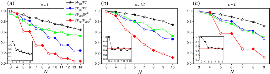
In Fig. 15 the overlaps of and with the ground state of the AFHC of Eq. (1) are shown. These overlaps largely confirm the picture discussed in the previous paragraph. For small and especially larger the model has a slight advantage over the VBS ground state, but then its overlap drops off quickly with . Again the overlaps are slightly better for even than for odd . The overlap of on the other hand is much less dependent on and also drops off slower with . This shows that local quantum entanglement is important for any and , while the Néel-type order of is relevant for large and small . The overlap of the two ground states and is also plotted in Fig. 15. Interestingly, both models give very similar wavefunctions up to , as can be concluded from the large overlap values.
To improve on the quality of the variational approximation both the and VBS models were simultaneously taken into account, by forming a trial state as a linear combination of the two corresponding wavefunctions, namely the optimal wavefunction (the notation always implies normalization). Its overlap with the AFHC ground state is also plotted in Fig. 15 for the optimal combination of the variational parameters and . The overlap improves in comparison with the two individual wavefunctions but still decreases with , with a weak dependence on . In the insets of Fig. 15 the optimal ratio is plotted. The overlap decrease with shows the importance of the VBS state for longer chains. It generally increases with , and the model gains more weight as the increase of makes the AFHC ground state more Néel ordered and less entangled.
Comparing the approximation of the ground state energy (Fig. 14) with the overlap of the ground state wavefunction (Fig. 15) for the VBS model, the former hardly worsens with , while the overlap of the wavefunctions decreases. This is due to the fact, that the overlap of the VBS model wavefunction with the AFHC wavefunctions of other low lying energy levels is still significant. Hence the VBS wavefunction mostly mixes with the low lying AFHC energy levels.
IX Summary and Conclusions
In this work the structure of the lowest excitations in AFHCs of relatively short length but relatively large spin magnitude has extensively been studied by contrasting the results of a broad array of theoretical tools and approaches. The results of this paper are of relevance from at least three perspectives.
Quantum vs spatial fluctuations. First of all, the findings further our understanding of the physics in the AFHC model. It has been demonstrated that there is a distinctive even-odd effect in the dependence of the lowest energies in each total-spin sector on or the band in short chains. The effect is markedly different to the established even-odd effect in long chains, which is well understood in terms of the quantum edge-spin picture; the arguments were given in Sec. IV.3. The different physics found in these two regimes justifies a distinction into short and long chains, which represents a major finding of this work. The described even-odd effect manifests itself in the antiferromagnetic region of the -band spectrum (low ), but not in the ferromagnetic part (high ). In the antiferromagnetic region even-odd effects can also be noticed e.g. in the ground-state spin, the spin density, and the nearest-neighbor correlation functions. These are however straightforwardly explained by the different symmetry properties of even and odd chains. The even-odd effect focused on in this work in contrast is not as trivially traced back to the different symmetry properties of even and odd chains.
To elucidate the physics giving rise to this effect, different models were investigated, and the AFHC model was firstly compared to the model. Phenomenologically, the model appeared as a promising candidate since it naturally produces an energy dependence and an -band structure, as approximately observed in short AFHCs (Fig. 1). While for odd chains the model describes the band surprisingly well in the full range of values, with a slight renormalization of the slope or the effective gap , it fails to do so for even chains. The deviation is most pronounced in the antiferromagnetic region for , which is the even-odd effect, but also in the ferromagnetic region the deviation is significant. For even-membered antiferromagnetic Heisenberg rings the energies predicted by the model were previously shown to become more accurate the larger , and the model was hence considered (semi-)classical in nature.[31] Our results on the AFHC correct this view and point to the fact that the main characteristics of the model is the neglect of spatial fluctuations or implicit assumption of an infinite correlation length, which consistently explains our findings. For instance, the spin densities are more homogeneous in odd than even chains suggesting a better accuracy of the predictions in the odd chains. Also, that the model reproduces energies and transition matrix elements extremely well for rings is now expected from the fact that in rings the -band states exhibit homogeneous spin densities by symmetry. These trends for rings, odd and even chains also manifest themselves in the ferromagnetic region, as characterized by the slope . For rings one finds , which coincides with the prediction of the model (), while for chains (with ) holds, with the larger discrepancy for the even chains.
The predictions of the O(3) NLSM for short AFHCs were also analyzed. Interestingly, with neglected spatial fluctuations the model is reproduced, which underpins the role of spatial fluctuations and establishes the theoretical basis of the model. More importantly, the analysis demonstrated that the even-odd effect is not easily reconciled within the NLSM. It in fact showed that the usual assumption of describing Néel order and uniform canting as separate, weakly coupled degrees of freedom, which is exploited in or is even at the heart of many theories such as bosonization, hydrodynamic theories, or those based on the NLSM, fails in short chains. In particular, it demonstrated that the even-odd effect is distinct from the even-odd effects due to the quantum edge-spin model established for long chains. The latter was furthered by an analysis of the VBS wavefunctions for AFHC systems. As e.g. demonstrated by the analysis of the spin densities and correlations, differences between half-integer and integer spin chains are small for short chains. The VBS results thus suggest that in short chains (with ) the integer-spin VBS part in the total VBS wavefunction is more relevant to the physics than the additional half-integer spin VBS part present in half-integer spin chains. Somewhat surprisingly it was found that the VBS and wavefunctions approximate the exact wavefunctions nearly equally well (or equally poor) for small chains with relatively large spin magnitudes . The and the quantum VBS models capture different aspects of the wavefunctions; each model has hence its strengths and weaknesses with no clear advantage for one over the other.
Finally, the AFHC was also analyzed in the classical limit. The classical model describes the general trends and in particular the even-odd effect very nicely, as shown by the numerical results, leaving little doubt that it captures the essential physics. As main result it demonstrates the importance of spatial fluctuations in the even-odd effect. Qualitatively, the even-odd effect can be related to the spatial inhomogeneities introduced by the spins at the edges and their larger response to weak applied magnetic fields in the case of even chains [i.e. a smaller slope ]. At a quantitative level significant deviations remain unexplained, which reflects the fact that for the considered spin magnitudes the classical limit is not yet reached and quantum fluctuations still play a significant role. As a striking, yet so far unexplained consequence, the band of odd quantum chains is well described by the model, which predicts the slope better than the classical model in Fig. 9(b).
Physical regimes in the AFHC model. Having established fundamentally different behavior for short and long chains, the question arises where the crossover between these regimes is located. It was first argued by Haldane that in the thermodynamic limit determines the physical behavior, leading to a gap in the excitation spectrum for integer , while half-integer spin chains have a linearly dispersing excitation spectrum.[12, 13, 14] In the framework of the renormalization group treatment of the NLSM in Eq. (17) both integer and half-integer spin chains in fact show the same increase of the dimensionless coupling constant in the weak-coupling expansion.[87, 88] The length scale at which a weak-coupling expansion breaks down is given by irrespective of being integer or half-integer.[87, 88] For integer spin chains this implies a gap proportional to the inverse cut-off length . For half-integer spin chains the topological term leads to a different physical behavior which resembles that of the chain, i.e., a gapless critical behavior. While this difference is always observed in the thermodynamic limit at small fields, it is important to realize that any relevant energy scale such as fields or finite-size gaps will lead to a different renormalization flow. The physical behavior is then determined by the largest energy scale or equivalently the smallest length scale.
In the case of finite chains there are several relevant length scales (energy scales), such as the chain length or the correlation length due to finite fields in Eq. (38). The length scale corresponding to the breakdown of the weak-coupling expansion is
| (43) |
which corresponds to the correlation length in integer spin chains. Two fundamentally different physical regimes can be identified (in zero field and temperature):
(1) : This regime corresponds to the most studied case of the thermodynamic limit, where the famous difference between integer and half-integer spin is observed. For finite chains with (long chains) it is possible to clearly see the characteristic features of the thermodynamic limit by finite-size scaling (in the form of characteristic corrections). The behavior can be well described by continuous quantum field theories; hence we call this case the ”renormalized continuous quantum regime”.
(2) : This regime of short chains was the main topic of this paper. The finite-size effects dominate and the physical behavior is sensitive to the boundary condition and the geometry of the finite cluster, which leads to the even-odd effect. It is fundamentally impossible to connect the unique behavior in this regime analytically to the thermodynamic limit by finite-size scaling. Since many of the features are correctly reproduced by the corresponding classical model but quantum effects are still important (see below), we call this case the ”bounded quantum-classical regime”.
In finite magnetic fields the correlation length comes also into play. The above two regimes are present at low fields, or . The field gives rise however to a further regime where , which we call the ”ferromagnetic regime”. It is dominated by a relatively large magnetic field or large magnetization , and both short and long chains enter it under these conditions, obliterating the distinction between the two low-field regimes. Our numerical results show that the correlations are dominated by the trend to align all spins with the total spin. This behavior is continuously connected to the ferromagnetic region, and can be best described by a hydrodynamic theory or by spin waves, which give analogous results.[80, 89] The behavior shows no fundamental difference between even and odd nor between integer and half-integer . For completeness it is mentioned that in addition there is also a finite temperature regime with smallest length scale , which is however not considered in this paper.

The above considerations demonstrate that the crossover from short to long is characterized by the length , which depends on and thus describes a boundary line as sketched in Fig. 16. This plot was not completely traced out by the numerical results (for obvious limitations in computational power), but the present work provides strong pieces of evidence for its validity. For instance, since , the region of short chains is not reachable in chains, which is perfectly consistent with Fig. 3, where the variation of with is distinctly different for , and the absence of the even-odd effect in the chain as shown in Sec. V. For the short-chain region starts to become available, but the short-chain behavior may be realized only approximately, which is consistent with e.g. Fig. 5. For , however, the short-chain region is already available for significant chain lengths. This trend with is also consistent with the notion that in the VBS picture the half-integer spin part in the VBS wavefunction (when present) becomes less and less relevant the larger is, such that the physics is related to the integer spin part. Lastly, the analysis of the classical chain model showed that for large the short-chain behavior is indeed present also in chains with large, but finite , as expected from Eq. (43). In particular, the slope is suppressed for large even in the low field limit, though only in a small range of fields . Generally, the short-chain region becomes more accessible the larger and the smaller is, while the long-chain region is accessible for relatively small and large .
The region of small and large or long chains has been studied in great detail in the past and the physics can be summarized as the renormalized continuous quantum regime. For short chains, in contrast, it was demonstrated in this paper that many of the features, such as the spatial fluctuations, are qualitatively explained by the corresponding classical model, and that in this sense short chains are classical. However, for experimentally accessible spin magnitudes quantum fluctuations are clearly not negligible, as demonstrated e.g. by the slow convergence of the quantum results to the classical limit or the significant overlap of the wavefunctions with the VBS states. A further example is the superior performance of the model over the classical model for the odd chains, and it remains surprising that the slope for odd chains follows the prediction of well although the local correlations do not. Short chains hence show both classical and quantum aspects, depending on the feature one is looking at, and in this sense blur the distinction between classical and quantum physics. Hence we use the notation ”bounded quantum-classical regime” for this case. Remarkably, in this regime the physical behavior becomes largely independent of and , i.e., is generic.
Implications for spin clusters in general. At this point our results are of relevance also from a broader, fundamental perspective. A diagram which at first sight is very similar to that in Fig. 16 was proposed a decade ago based on studies on antiferromagnetic Heisenberg rings of relatively small size but with relatively large spin magnitudes .[31] It was in particular demonstrated that the -band picture and the energies and matrix elements calculated with become more accurate the larger and the smaller is.[31, 54] That is, the large -small region was (erroneously) linked in this and subsequent works to the validity of the model, which lead to some inconsistencies.[11] In the present work, the situation is rectified by identifying the (classical) spatial fluctuations as the characterizing feature in this regime. Both the ”small” rings and short chains are apparently in the bounded quantum-classical regime. However, for rings additionally the model is an excellent approximation because of the symmetry-induced homogeneous spin densities in their -band states. For chains, in contrast, the model is less appropriate.
The present work thus states more precisely the distinctive behavior of small rings anticipated in Ref. 31 and puts it for the chain systems, through a very detailed numerical and theoretical analysis, on a solid basis. The results lend credit to the idea that the two distinctive regimes are in fact generic and present not only in rings and chains, but also in other and potentially many small antiferromagnetic Heisenberg clusters, since one could generally expect that spatial fluctuations dominate over quantum fluctuations in these systems. For the calculation of the quantum fluctuations introduced by magnetic anisotropy terms powerful theoretical tools exist.[90] In contrast, for the effects of the antiferromagnetic Heisenberg interactions in relatively small lattices, a satisfying quantitative theory which takes into account the relevant effects, i.e., treats the (classical) spatial fluctuations correctly and introduces the quantum effects, appears to be missing at the moment. Developing it should be an attractive challenge for the future.
It is finally mentioned that clusters of a dozen exchange-coupled spin centers with relatively large spin magnitudes are currently of high experimental relevance. An abundance of examples is provided by the class of molecular nanomagnets,[91] which through synthetic chemistry has generated hundreds of magnetic molecules with different arrangements of the metal centers. The number of spin centers ranges from 4 to a current maximum of 84, and the spin magnitudes are typically , 2, and 5/2 for transition metal clusters. Furthermore, the emerging field of the artificially engineered spin clusters can be expected to provide many further attractive experimental systems.[8, 9, 10] The key findings in this work should be of fundamental importance to a variety of currently studied experimental systems, where mesoscopic effects are very important, and very promising applications go hand in hand with interesting many-body effects.
Acknowledgements.
The authors thank Ian Affleck and Frank Pollmann for many highly useful comments and fruitful discussions on the topic. Partial funding by the Deutsche Forschungsgemeinschaft is thankfully acknowledged.Appendix A Spin coupled basis
In view of the SU(2) symmetry of Eq. (1) it is convenient to perform numerical work directly in a basis of eigenstates of the total spin operator . Since this is rarely done in the area of quantum spin systems, some details shall be given here. The general procedure is given by Racah’s methods and the irreducible tensor operator (ITO) techniques.[4]
In this paper the spin coupling scheme was used where at first the first two spins are coupled, and then successively the next spin to the previous ones: . This yields the SU(2) invariant basis states with intermediate spin quantum numbers , , , . This basis is exploited by expressing the Hamiltonian in terms of ITOs.[4]
The ITO of rank associated to the spin center has components with . Coupling ITOs of different rank and different spins is generally achieved through
| (44) | |||||
where the have to be populated according to the spin coupling scheme and the intermediate spin quantum numbers. The tensor product of two ITOs thereby reads
| (45) |
By repeated application of Eq. (45) the coupling of the ITOs in Eq. (44) can be recast into a sum over the products of single-spin ITOs and Clebsch-Gordon coefficients .
For pairwise interactions we introduce the notation , indicating a many-spin ITO in Eq. (44) with corresponding values and for the single-spin ITOs and and all if . Note that the elementary ITOs are defined as
| (46) |
while is the identity. For a Heisenberg system only the ITO representation of is needed, which is
| (47) |
The parent Hamiltonians for the VBS wavefunctions in Eqs. (40) and (41) include also higher-order coupling terms , which lead to higher order polynomials of the ITOs and respectively, e.g. . These polynomials can be successively reduced by the building up principle [92]
| (48) |
with
| (52) | |||||
The reduced matrix elements are given by
| (53) |
The biquadratic term then becomes[93]
For the VBS parent Hamiltonian also the term is needed for which we obtain
| (55) | |||||
Finally, the VBS parent Hamiltonians in terms of ITOs read:
| (56) | |||||
| (57) | |||||
Appendix B Iterative construction of VBS wavefunctions
VBS wavefunctions can be calculated in the spin coupled basis using iteration. For a dimer of two spins the VBS wavefunction is known in the spin coupled basis. It is degenerate in , and the maximal is . The wavefunctions are for total spin in an obvious notation, and go up to for total spin . If it is known what happens when a further spin is attached, i.e., if the VBS wavefunction for an open chain of 3 spins with spin is known, then by iteration the VBS wavefunction for any chain of length can be calculated. In each iteration step the corresponding basis vectors are extended by one lattice site, i.e. from to . The method finds the unnormalized coefficients for a VBS wavefunction in the spin coupled basis, and the resulting wavefunction has therefore to be normalized after completion of the iteration.
For an VBS chain [Figs. 13(c), (d)] the iteration reads
| (58) | |||||
The basis functions of and are orthogonal. The number of relevant basis functions for the chain grows with like the Fibonacci numbers. For an VBS chain [Figs. 13(g), (h)] one finds
| (59) | |||||
and for an VBS chain
| (60) | |||||
For the dimerized valence bond function [Figs. 13(e), (f)] with only one singlet bond between the first two spins one obtains
| (61) | |||||
and for the dimerized valence bond function with two singlet bonds between the first two spins holds
| (62) | |||||
Appendix C Technical details in the derivation of the O(3) NSLM
In this appendix the O(3) NSLM is derived in detail. With the decomposition (16) the action in (15) is evaluated. First, expanding the term up to order :
| (63) | |||||
Differences of the Néel fields can be approximated by derivatives which allow to write . Then up to a constant term:
| (64) | |||||
The alternating term requires a careful treatment of the boundary conditions. For periodic boundary conditions and even the term can be neglected as can be seen by writing and which directly yields
| (65) |
For open boundary conditions additional boundary terms remain. Discussion of these terms is left for later and periodic boundary conditions are considered now. Introducing and taking the continuum limit:
| (66) |
Next, the imaginary part in Eq. (15) is evaluated. The Berry phase is antisymmetric under inversion , hence
| (67) | |||||
In Sec. IV the first term in Eq. (67) is of ”topological” significance. The second one in contrast enters in the classical equation of motion.
Up to an additive constant the total action reads
| (68) | |||||
Completing the square the functional integration over can be performed, giving . Thus, the field generates rotations on . Note that the constraint is automatically fulfilled. Overall normalization constants are left out. Finally, the O(3) NSLM is generated, with a term as the effective action for the Heisenberg chain in the large limit, see Eq. (17).
Finally, Eq. (65) is considered for open boundaries. Using and the following boundary terms are obtained:
These terms have a scaling dimension of one order higher than the bulk terms in the action in Eq. (17). Note that they are of the same order as the higher order terms in the Euler-Maclaurin sum formula that occur when going from the discrete sum to the continuum integral, see Eq. (66). It is assumed that these terms are small.
References
- [1] E. Manousakis, Rev. Mod. Phys. 63, 1 (1991).
- [2] A. Auerbach, Interacting Electrons and Quantum Magnetism (Springer-Verlag, New York, 1998).
- [3] C. Lhuillier and P. Sindzingre, Quantum Properties of Low-Dimensional Antiferromagnets (Kuyshu University Press, Kuyshu, 2002).
- [4] A. Bencini and D. Gatteschi, Electron Paramagnetic Resonance of Exchange Coupled Systems (Springer-Verlag, Heidelberg, 1990).
- [5] A. Furrer and O. Waldmann.
- [6] D. Gatteschi, A. Caneschi, L. Pardi, and R. Sessoli, Science 265, 1054 (1994).
- [7] O. Waldmann, Coord. Chem. Rev. 249, 2550 (2005a).
- [8] C. F. Hirjibehedin, C. P. Lutz, and A. J. Heinrich, Science 312, 1021 (2006).
- [9] T. Jamneala, V. Madhavan, and M. F. Crommie, Phys. Rev. Lett. 87, 256804 (2001).
- [10] A. Enders, R. Skomski, and J. Honolka, J. Phys.: Condens. Matter 22, 433001 (2010).
- [11] N. P. Konstantinidis, A. Sundt, J. Nehrkorn, A. Machens, and O. Waldmann, J. Phys. Conf. Ser. 303, 012003 (2011).
- [12] F. D. M. Haldane, Phys. Lett. A 93, 464 (1983a).
- [13] F. D. M. Haldane, Phys. Rev. Lett. 50, 1153 (1983b).
- [14] I. Affleck, J. Phys. Cond. Matt. 1, 3047 (1989).
- [15] S. Qin, T.-K. Ng, and Z.-B. Su, Phys. Rev. B 52, 12844 (1995).
- [16] J. Sirker, S. Fujimoto, N. Laflorencie, S. Eggert, and I. Affleck, J. Stat. Mech. P02015 (2008).
- [17] F. Anfuso and S. Eggert, Europhys. Lett. 73, 271 (2006a).
- [18] S. Eggert, I. Affleck, and M. D. P. Horton, Phys. Rev. Lett. 89, 047202 (2002).
- [19] S. T. Ochsenbein, O. Waldmann, A. Sieber, G. Carver, R. Bircher, H. U. Gudel, R. S. G. Davies, G. A. Timco, R. E. P. Winpenny, H. Mutka, et al., Europhys. Lett. 79, 17003 (2007).
- [20] S. T. Ochsenbein, F. Tuna, M. Rancan, R. S. G. Davies, C. A. Muryn, O. Waldmann, R. Bircher, A. Sieber, G. Carver, H. Mutka, et al., Chem. Eur. J. 14, 5144 (2008).
- [21] A. Ghirri, A. Candini, M. Evangelisti, M. Affronte, S. Carretta, P. Santini, G. Amoretti, R. S. G. Davies, G. Timco, and R. E. P. Winpenny, Phys. Rev. B 76, 214405 (2007).
- [22] A. Bianchi, S. Carretta, P. Santini, G. Amoretti, T. Guidi, Y. Qiu, J. R. D. Copley, G. Timco, C. Muryn, and R. E. P. Winpenny, Phys. Rev. B 79, 144422 (2009).
- [23] Y. Furukawa, K. Kiuchi, K. I. Kumagai, Y. Ajiro, Y. Narumi, M. Iwaki, K. Kindo, A. Bianchi, S. Carretta, G. A. Timco, et al., Pyhs. Rev. B 78, 092402 (2008).
- [24] S. Piligkos, E. Bill, D. Collison, E. J. L. McInnes, G. A. Timco, H. Weihe, R. E. P. Winpenny, and F. Neese, J. Am. Chem. Soc. 129, 760 (2007).
- [25] E. Micotti, Y. Furukawa, K. Kumagai, S. Carretta, A. Lascialfari, F. Borsa, G. A. Timco, and R. E. P. Winpenny, Phys. Rev. Lett. 97, 267204 (2006).
- [26] T. Guidi, J. R. D. Copley, Y. Qiu, S. Caretta, P. Santini, G. Amoretti, G. Timco, R. E. p. Winpenny, C. L. Dennis, and R. Caciuffo, Phys. Rev. B 75, 014408 (2007).
- [27] J. J. Henderson, C. M. Ramsey, E. del Barco, T. C. Stamatatos, and G. Christou, Phys. Rev. B 78, 214413 (2008).
- [28] P. W. Anderson, Phys. Rev. 86, 694 (1952).
- [29] B. Bernu, C. Lhuillier, and L. Pierre, Phys. Rev. Lett. 69, 2590 (1992).
- [30] J. Schnack and M. Luban, Phys. Rev. B 63, 014418 (2000).
- [31] O. Waldmann, Phys. Rev. B 65, 024424 (2001).
- [32] O. Waldmann, T. Guidi, S. Carretta, C. Mondelli, and A. L. Dearden, Phys. Rev. Lett. 91, 237202 (2003).
- [33] O. Waldmann, C. Dobe, H. U. Güdel, and H. Mutka, Phys. Rev. B 74, 054429 (2006).
- [34] J. Ummethum, J. Nehrkorn, S. Mukherjee, N. B. Ivanov, S. Stuiber, T. Strässle, P. L. W. Tregenna-Piggott, H. Mutka, G. Christou, O. Waldmann, et al., Phys. Rev. B 86, 104403 (2012).
- [35] T. Guidi, S. Carretta, P. Santini, E. Liviotti, N. Magnani, C. Mondelli, O. Waldmann, L. K. Thompson, L. Zhao, C. D. Frost, et al., Phys. Rev. B 69, 104432 (2004).
- [36] J. Schnack, M. Luban, and R. Modler, Europhys. Lett. 56, 863 (2001).
- [37] M. Exler and J. Schnack, Phys. Rev. B 67, 094440 (2003).
- [38] V. O. Garlea, S. E. Nagler, J. L. Zarestky, C. Stassis, D. Vaknin, P. Kögerler, D. F. McMorrow, C. Niedermayer, D. A. Tennant, B. Lake, et al., Phys. Rev. B 73, 024414 (2006).
- [39] O. Waldmann, Phys. Rev. B 75, 012415 (2007).
- [40] T. Kennedy, J. Phys. Condens. Matter 2, 5737 (1990).
- [41] M. Hagiwara, K. Katsumata, I. Affleck, B. I. Halperin, and J. P. Renard, Phys. Rev. Lett. 65, 3181 (1990).
- [42] S. J. Glarum, S. Geschwind, K. M. Lee, M. L. Kaplan, and J. Michel, Phys. Rev. Lett. 67, 1614 (1991).
- [43] E. S. Sørensen and I. Affleck, Phys. Rev. B 49, 15771 (1994).
- [44] T.-K. Ng, Phys. Rev. B 50, 555 (1994).
- [45] J. Lou, S. Qin, T.-K. Ng, and Z. Su, Phys. Rev. B 65, 104401 (2002).
- [46] E. Lieb and D. Mattis, J. Math. Phys. 3, 749 (1962).
- [47] O. Waldmann, Phys. Rev. B 61, 6138 (2000).
- [48] N. P. Konstantinidis, Phys. Rev. B 72, 064453 (2005).
- [49] I. Affleck, T. Kennedy, E. H. Lieb, and H. Tasaki, Phys. Rev. Lett. 59, 799 (1987).
- [50] I. Affleck, T. Kennedy, E. H. Lieb, and H. Tasaki, Comm. Math. Phys. 115, 477 (1988).
- [51] S. Eggert and I. Affleck, Phys. Rev. B 46, 10866 (1992).
- [52] B. Bernu, P. Lecheminant, C. Lhuillier, and L. Pierre, Phys. Rev. B 50, 10048 (1994).
- [53] O. Waldmann, Phys. Rev. B 71, 094412 (2005b).
- [54] A. Chiolero and D. Loss, Phys. Rev. Lett. 80, 170 (1998).
- [55] E. Fradkin and M. Stone, Phys. Rev. B 38, 7181 (1988).
- [56] E. Witten, Nucl. Phys. B 223, 422 (1983).
- [57] J. Dai and W. M. Zhang, Phys. Rev. Lett. 95, 167205 (2005).
- [58] A. B. Zamolodchikov and A. B. Zamolodchikov, Ann. Phys. 120, 253 (1979).
- [59] I. Affleck and F. D. M. Haldane, Phys. Rev. B 36, 5291 (1987).
- [60] R. Shankar and N. Read, Nucl. Phys. B 336, 457 (1990).
- [61] A. B. Zamolodchikov and A. B. Zamolodchikov, Nucl. Phys. B 379, 602 (1992).
- [62] W. Bietenholz, A. Pochinsky, and U. J. Wiese, Phys. Rev. Lett. 75, 4524 (1995).
- [63] E. Lieb, T. Schultz, and D. Mattis, Ann. Phys. NY 16, 407 (1961).
- [64] C. Grosche and F. Steiner, Z. Phys. C 36, 699 (1987).
- [65] E. Rabinovici, A. Schwimmer, and S. Yankielowicz, Nucl. Phys. B 248, 523 (1984).
- [66] B. Normand, X. Wang, X. Zotos, and D. Loss, Phys. Rev. B 63, 184409 (2001).
- [67] F. Maier and D. Loss, Phys. Rev. B 64, 224411 (2001).
- [68] J. Lou, S. Qin, and C. Chen, Phys. Rev. Lett. 91, 087204 (2003).
- [69] M. Bortz, M. Karbach, I. Schneider, and S. Eggert, Phys. Rev. B 79, 245414 (2009).
- [70] I. Affleck, D. Gepner, H. Schulz, and T. Ziman, J. Phys. A 22, 511 (1989).
- [71] S. Eggert and I. Affleck, Phys. Rev. Lett. 75, 934 (1995).
- [72] S. Rommer and S. Eggert, Phys. Rev. B 62, 4370 (2000).
- [73] S. Lounis, P. H. Dederichs, and S. Blügel, Phys. Rev. Lett. 101, 107204 (2008).
- [74] P. Politi and M. G. Pini, Phys. Rev. B 79, 012405 (2009).
- [75] M. E. Fisher, Am. J. Phys. 32, 343 (1964).
- [76] G. S. Joyce, Phys. Rev. 155, 478 (1967).
- [77] D. Coffey and S. A. Trugman, Phys. Rev. Lett. 69, 176 (1992).
- [78] N. P. Konstantinidis, Phys. Rev. B 76, 104434 (2007).
- [79] N. P. Konstantinidis and M. Luban, unpublished.
- [80] S. Eggert, O. F. Syljuåsen, F. Anfuso, and M. Andres, Phys. Rev. Lett. 99, 097204 (2007).
- [81] F. Anfuso and S. Eggert, Phys. Rev. Lett. 96, 017204 (2006b).
- [82] A. Wollny, E. C. Andrade, and M. Vojta, Phys. Rev. Lett. 109, 177203 (2012).
- [83] E. S. Sørensen and I. Affleck, Phys. Rev. Lett. 71, 1633 (1993).
- [84] D. P. Arovas, A. Auerbach, and F. D. M. Haldane, Phys. Rev. Lett. 60, 531 (1988).
- [85] K. S. D. Beach and A. W. Sandvik, Nucl. Phys. B 750, 142 (2006).
- [86] S. Rachel, Europhys. Lett. 86, 37005 (2009).
- [87] A. Polyakov, Phys. Lett. 59b, 79 (1975).
- [88] E. Fradkin, Field Theories of Condensed Matter Systems (Addison-Wesley Publishing Company, University of Minnesota, 1991).
- [89] S. Shinkevich, O. F. Syljuåsen, and S. Eggert, Phys. Rev. B 83, 054423 (2011).
- [90] L. Gunther and B. Barbara, Quantum Tunneling of Magnetization (Kluwer, Dordrecht, 1995).
- [91] D. Gatteschi, R. Sessoli, and J. Villain, Molecular Nanomagnets (Oxford University Press, Oxford, 2006).
- [92] R. P. Bickerstaff and B. G. Wybourne, J. Phys. A: Math. Gen. 9, 1051 (1976).
- [93] J. J. Borrás-Almenar, J. M. Clemente-Juan, E. Corondo, and B. S. Tsukerblat, Inorg. Chem. 38, 6081 (1999).