Degrees of Freedom of the -User Rank-Deficient MIMO Interference Channel
Abstract
We provide the degrees of freedom (DoF) characterization for the -user multiple-input multiple-output (MIMO) interference channel (IC) with rank-deficient channel matrices, where each transmitter is equipped with antennas and each receiver with antennas, and the interfering channel matrices from each transmitter to the other two receivers are of ranks and , respectively. One important intermediate step for both the converse and achievability arguments is to convert the fully-connected rank-deficient channel into an equivalent partially-connected full-rank MIMO-IC by invertible linear transformations. As such, existing techniques developed for full-rank MIMO-IC can be incorporated to derive the DoF outer and inner bounds for the rank-deficient case. Our result shows that when the interfering links are weak in terms of the channel ranks, i.e., , zero forcing is sufficient to achieve the optimal DoF. On the other hand, when , a combination of zero forcing and interference alignment is in general required for DoF optimality. The DoF characterization obtained in this paper unifies several existing results in the literature.
Index Terms:
Degrees of freedom, MIMO interference channel, rank deficiency, zero forcing, interference alignment.I Introduction
Finding the information-theoretic capacity of the general Gaussian interference channel (IC) is a long-standing open problem [1]. On the other hand, the characterizations of the degrees of freedom (DoF) value, a parameter that provides the first-order capacity approximation at the asymptotically high signal-to-noise ratio (SNR), have been successfully accomplished in various settings [2, 3, 4, 5, 6, 7, 8, 9, 10]. In particular, for interference channels with more than two users and hence each receiver is interfered by more than one interfering sources, the technique known as interference alignment has been shown to achieve higher DoF than previously believed [4, 5, 6, 7]. More recently, for the -user IC with antennas at each transmitter and antennas at each receiver, a novel concept of “subspace alignment chains” was introduced in [10], where ideally each transmitted signal subspace is aligned with another interference subspace at both undesired receivers and an alignment chain is formed, and the finite length of the alignment chain ultimately limits the attained DoF value. Furthermore, for the DoF outer bound proof in [10], a technique termed “onion peeling” has been introduced, where an equivalent channel with layered structure was obtained by applying change of basis operations at the transmitters and receivers. As such, it helps determining the appropriate genie signals to be provided to each receiver for deriving the outer bounds.
The aforementioned works for DoF characterizations have all assumed full-rank channel matrices. Such an assumption is valid in rich scattering environment with sufficient number of signal paths. However, in some practical scenarios, the communication channel matrices may be rank deficient due to poor scattering and hence with only very few signal paths. There are only a few works reported on the DoF characterizations of rank-deficient multiple-input multiple-output IC (MIMO-IC) [11, 12, 13]. In [11], under the assumption that all channel matrices have the same rank, an achievable DoF value was obtained for the -user time-varying IC. The achievable scheme proposed therein is based on either zero forcing or interference alignment, whichever gives a higher DoF value. In [12], the authors investigated the DoF of the -user and -user rank-deficient MIMO-IC. While the optimal DoF value has been obtained for the general 2-user scenario, only the symmetric setup where all terminals are equipped with antennas was considered for the 3-user case. Later, the result in [12] was extended to the symmetric -user MIMO-IC [13], where all direct channels have rank and all cross channels have rank .
In this paper, we investigate the DoF of the -user rank-deficient MIMO-IC where each transmitter is equipped with antennas and each receiver with antennas. All the direct channel matrices are of rank , and the interfering channel matrices from each transmitter to the other two receivers are of ranks and , respectively. Our model is more general than that studied in [12] since the transmitters and receivers may have different number of antennas and , respectively. It is worth mentioning that such a generalization is nontrivial due to the more complicated relations between the channel ranks and the number of transmit and receive antennas, which makes the derivations of the outer and inner bounds much more challenging. In fact, even for the full-rank case, the extension of the DoF result for the 3-user MIMO-IC from the setup [4] to the more general case [10] is highly involved and requires much more sophisticated techniques such as subspace alignment chains and onion peeling, as discussed previously. By adopting spatial extension for the inner bound to deal with non-integer DoF values [10], we provide a complete DoF characterization for all possible settings of the -user rank-deficient MIMO-IC parameterized by . Specifically, with spatial extension, the DoF achievability is firstly established for a larger network obtained by virtually scaling the number of antennas and channel ranks so that the DoF are integers. By normalizing with the same factor, the desired result for the original setup is then obtained. As argued in [10] and [14], such a technique is justified by the fact that for every wireless network where the DoF characterizations are available, the DoF result is unaffected by spatial extension and then DoF normalization. Therefore, it has been conjectured that similar to time/frequency dimension, the DoF of a wireless network scale with the proportional scaling of spatial dimension [10]. On the other hand, compared to time or frequency extensions, spatial extension makes it easier to deal with non-integer DoF values without having to deal with the added complexity of diagonal or block diagonal channel structures.
To achieve the maximum possible DoF value, intuitively, one should zero force as many interfering links as possible. One distinguishing feature of the rank-deficient MIMO-IC, as compared to the full-rank counterparts, is that both the left and right null space of the interfering channel matrices are non-empty, and hence should be utilized for zero forcing purposes. Therefore, a critical step for achieving the optimal DoF for rank-deficient MIMO-IC is to appropriately exploit the rank deficiency of the interfering channel matrices. To this end, we first transform the original fully-connected rank-deficient MIMO-IC into an equivalent partially-connected full-rank MIMO-IC. This in effect extracts the rank-deficiency of the interfering channel matrices embedded in all antennas to a subset of antennas so that the corresponding interfering links are nullified. As such, existing techniques developed for full-rank MIMO-IC, such as “onion peeling” based on the equivalent layered channel structure and subspace alignment chains, can be incorporated to facilitate the derivations of the DoF outer and inner bounds.
The outer bound is derived with the genie-aided signaling technique based on the developed equivalent layered channel model. For the achievability, a two-layered linear processing scheme is proposed, with zero forcing in the inner layer and a block-diagonal precoding and interference cancelation, if necessary, in the outer layer. The use of block-diagonal precoding, together with the zero forcing operation in the inner layer, ensures that each information-bearing symbol only interferes a particular group of receive antennas at the undesired receivers, which in turn makes interference cancelation possible. When the interfering links are weak in terms of the channel ranks, i.e., , zero forcing together with a random block-diagonal precoding is sufficient to achieve the optimal DoF; whereas when , the block-diagonal precoding in the outer layer must be carefully designed so that interference alignment is achieved, i.e., in this case, a combination of zero forcing and interference alignment is in general required to achieve the optimal DoF value.
Notations: Scalars are denoted by italic letters. Boldface lower- and upper-case letters denote vectors and matrices, respectively. represents the space of complex matrices. For a matrix , and denote its transpose and rank, respectively. The null space of is denoted by , and hence its left null space can be represented as . denotes a subspace spanned by the columns of . denotes the number of elements in vector . For a real number , denotes the smallest integer not less than and is the largest integer not greater than . represents any function such that .
II System Model
We consider a -user MIMO-IC where transmitter is intended to send message to receiver , . Each transmitter is equipped with antennas and each receiver has antennas. The signal received at receiver is given by
| (1) |
where denotes the direct channel matrix from transmitter to receiver , while , , denotes the interfering channel matrix from transmitter to receiver ; represents the received signal vector at receiver ; is the transmitted signal vector from transmitter ; and denotes the additive Gaussian noise vector.
Different from most existing works where full-rank channel matrices have been assumed, here we consider the more general scenario with possibly rank-deficient channel matrices, which may occur in the poor scattering communication environment with very few signal paths as illustrated in Section VII. Specifically, all the direct channel matrices are assumed to be of rank , and the interfering channel matrices and are of ranks and , respectively, as shown in Fig. 1. We then have . Note that the user index is interpreted modulo so that, e.g., user is the same as user . Due to small-scale fading, the channel matrices are assumed to be independent and randomly generated, where a random rank-deficient channel matrix of size with rank can be seen as a product of two full-rank generic matrices of size and . In the following, this channel model is expressed compactly as .

Denote by the average power constraint at each transmitter. The sum rate and the DoF follow from the standard definition in information theory. Further denote by the normalized DoF per user. Similar as [10], we define the spatially-normalized sum DoF as
| (2) |
Note that in (2), both the number of transmit and receive antennas and the ranks of the channel matrices are scaled by a factor , and the DoF are normalized by the same factor. While such a spatial extension is not necessary for the DoF outer bound, it is quite useful for the achievability result to deal with non-integer DoF values. We further denote by the spatially-normalized DoF per user, i.e., . For notational convenience, in the remaining part of this paper, we let , , and .
III Main Result and Discussions
Theorem 1
For the -user rank-deficient MIMO-IC , the spatially-normalized DoF value per user is given by
| (3) |
where .
The converse proof of Theorem 1 is based on the genie-aided signaling technique. The details are given in Section V with a preliminary step presented in Section IV. Note that the DoF converse is established for arbitrary values of , , , and , without the need for spatial extension. However, it can be verified that if the number of antennas and the ranks of the channel matrices are scaled by a factor , the outer bound for the DoF value would be scaled by the same factor as well. Therefore, the outer bound for the rank-deficient MIMO-IC scales with spatial dimension, and hence holds both with and without spatial normalization.
The achievability proof of Theorem 1 is based on a two-layered linear processing scheme, with zero forcing in the inner layer and block-diagonal precoding and interference cancelation in the outer layer. The details are given in Section VI.
Remark 1
Due to symmetry, the DoF value depends only on the sum of the ranks of the interfering channel matrices , instead of the individual ranks and . Therefore, a network parameterized by would have identical spatially-normalized DoF value as that parameterized by , for any valid .
Remark 2
For the rank-deficient MIMO-IC with fixed number of antennas, the DoF value is determined by either the rank of the direct link or that of the interfering links, depending on which one is the bottleneck. While the direct link affects the DoF via the simple quantity , the effect of the interfering links is complicated by the relations between , and . With , Fig. 2 plots versus for different values. It is observed that in the sufficiently low regime where either the transmitters (when ) or the receivers (when ) have enough number of antennas to zero force all interfering links, is solely limited by the rank of the direct links, i.e., ; otherwise, the interfering links will become the bottleneck and limit the maximum achievable . It is also observed for all , the DoF converges to the “half-cake” result [4] as approaches . On the other hand, with , higher DoF can be achieved, which is expected.

The DoF characterization given in Theorem 1 unifies several existing results in the literature.
III-1
In the extreme case when the interfering links vanish, i.e., , the model in (1) reduces to the -user independent point-to-point MIMO channels with the direct channel matrices having rank . In this case, it is well known that the DoF value per user is [15], which is equal to the value obtained by evaluating (3) with .
III-2
III-3
IV Equivalent Partially-Connected Full-Rank MIMO-IC
In this section, we present a preliminary step for the proof of Theorem 1, i.e., the conversion of the original fully-connected rank-deficient MIMO-IC to an equivalent partially-connected full-rank MIMO-IC by exploiting the rank deficiency of the interfering links and applying invertible linear transformations at the transmitters and receivers. While invertible linear transformations, or change of basis operations, do not affect the DoF, they create an equivalent channel such that the existing techniques developed for the full-rank MIMO-IC can be incorporated to facilitate the DoF study of the rank-deficient case.
Due to the reciprocity of linear transformations [16], without loss of generality, we assume in this section and in Section VI that , so that and . Furthermore, since different linear transformations are required for different interference levels, we distinguish the low- and high-interference cases, where the interference level is measured by the ranks of the interfering channel matrices as far as the DoF are concerned. Specifically, we have
- 1.
Low-interference case: .
- 2.
High-interference case: .
IV-A Low-Interference Case:
For the low-interference case with , we start with the design of the invertible linear transformation at receiver , which is based on the interfering channel matrices from transmitter and from transmitter . Based on which interfering links to be zero-forced, is partitioned as
| (6) |
where is designed so that it zero forces the signals from both interfering transmitters, i.e.,
| (7) |
Since , , and the channels are independent and randomly generated, with probability , we have
| (8) |
Therefore, the left null space of the concatenated matrix has dimension . The rows of are then selected to be the basis spanning this null space; and hence the size of is .
The two remaining blocks in are designed such that and zero force the interfering signals from transmitter and transmitter , respectively, i.e.,
| (9) |
Furthermore, since satisfying (7) also satisfies the zero-forcing conditions in (9), to ensure the invertibility of , the rows of are then selected from the left null space of , but not in the subspace spanned by the rows of . One possible design is to set to be the basis spanning the subspace . With , the dimension of the subspace where can be selected from is then given by . Therefore, the size of is given by . can be designed similarly and its size is . Under the assumption that the channel matrices are independent and randomly generated, it follows that with probability 1, the resulting matrix is of full rank, and hence invertible.
After at receiver is determined, we switch to the design of the invertible linear transformation at transmitter , which is partitioned as
| (10) |
where is designed so that it zero forces the interfering signals to both receiver and , i.e.,
| (11) |
The columns of are then selected to be the basis spanning the null space of the concatenated matrix in (11). Since and , we have
Therefore, the null space of the concatenated matrix in (11) has dimension and the size of is .
Next, the remaining two blocks and in are designed so that they zero force the interfering signals to receiver and receiver , respectively, i.e.,
| (12) |
Furthermore, since satisfying (11) also satisfies the zero-forcing conditions in (12), to ensure the invertibility of , the columns of are chosen from the null space of , but not in the subspace spanned by the columns of , e.g., can be set to be the basis spanning the subspace . With , the dimension of the subspace where the columns of can be selected from is then given by ; and hence is of size . A similar design for can be obtained and its size is . Under the assumption that the channel matrices are independent and randomly generated, the resulting matrix is of full rank, and hence is invertible.
Next, we derive the resulting channel model with the linear transformations and applied at the transmitters and receivers, respectively. Denote by the signal vector at transmitter before applying . Then the transmitted signal is given by . Based on the partition of in (10), is decomposed into head, middle and tail parts as , where the dimensions of the three blocks are respectively given by , , and . Further denote by the signal vector at receiver after applying linear transformation , i.e., , where is the received vector at receiver . By substituting with (1) and using , we get the input-output relationship after the linear transformations and as
| (13) |
where we have denoted by the interference vector at receiver . By substituting with (6) and with (10), can be written as , where
| (14) |
| (15) |
The above result shows that by applying the carefully designed linear transformations and , the middle antennas of receiver is interference-free, the head antennas are interfered only by the head antennas from transmitter via matrix , and the tail antennas are interfered only by the tail antennas from transmitter via matrix . Furthermore, since the channels are independent and randomly generated, with probability , the matrix and the matrix are both of full rank and hence invertible. Such an equivalent partially-connected full-rank MIMO-IC for the low-interference case is illustrated in Fig. 3.11 1 Note that only the residue interfering links are shown in Fig. 3 and in all similar plots hereafter. The direct links are omitted for conciseness.

IV-B High-Interference Case:
In the high-interference case where the interfering channel matrices have higher ranks, more residue interfering links than that shown in Fig. 3 are expected since in this case, the left and right nullspace of the interfering channel matrices from which the zero-forcing vectors are selected have smaller dimensions. As a result, and need to be designed differently from that given in the previous subsection. Firstly, at receiver is partitioned as
| (16) |
where , , and . The rows of and are selected from the left null spaces of and , respectively, but not in the intersection of these two null spaces. With , it can be verified that the specified number of rows for and can always be found. Furthermore, the central block is generated randomly. It then follows that the resulting matrix is full rank, and hence invertible.
With specified, we switch to the linear transformation at transmitter , which is partitioned as
| (17) |
where and are selected to be the basis spanning the null spaces of and , respectively. Note that since , we have . As a result, these two null spaces have empty intersection, and hence the columns of and are linearly independent. Next, the central block of is designed so that, together with the receiver matrix or , the interferences to a particular subset of antennas of receiver and receiver are zero-forced. More specifically, we need to have
| (18) |
Since is designed solely based on , it is independent of . Thus, we have
Similarly, we can obtain that . Since and are independent, we have
Therefore, the columns of can be chosen to be the basis spanning the null space of the concatenated matrix in (18) and its size is given by . It follows that the resulting matrices is full-rank and hence invertible.
Following similar analysis as for the low-interference case, the interference vector at receiver with transformations and can be obtained, where
| (19) |
| (20) | ||||
| (21) |
It can be obtained that the square matrices and defined above are both full-rank. Furthermore, the matrices and are both of full column rank. The equivalent partially-connected full-rank MIMO-IC with linear transformations and for the high-interference case is shown in Fig. 4.

V Information Theoretic DoF Outer Bound
In this section, we present the proof for the converse part of Theorem 1. First, with single-user bounding, we have
| (22) |
The remaining bounds in Theorem 1 are obtained by using the genie-aided signaling technique. To identify the appropriate side information to be provided by the genie, we use the equivalent partially-connected full-rank MIMO-IC developed in the preceding section. As pointed out in [10], since no claim to duality can be made a-priori for information theoretic DoF results, in principle, the two cases and need to be discussed separately. However, in this paper, we only present the detailed derivations for , or and , as the reciprocal channel can be dealt with similarly. Similar as in Section IV, we need to distinguish the low- and high-interference cases.
V-A Low-Interference Case:
For the low-interference case, the interfering links of the equivalent partially-connected full-rank MIMO-IC are plotted in Fig. 3. Since we are dealing with a converse argument, it follows by assumption that each receiver is able to decode and subtract out its desired signal. Consider the interference vector received by the head antennas of receiver . As given in (14), is a function of via the matrix . Since is full rank with probability , receiver is able to distinguish based on subject to the noise distortion. With a similar argument, receiver is also able to demodulate subject to the noise distortion after subtracting its desired signal. Hence, if a genie provides the signal to receiver , receiver should be able to decode all the three messages , and subject to the noise distortion. Let denote the rate for user and the sum rate of the three users. By Fano’s inequality, we have
| (23) |
where is true since receiver has only antennas, follows since conditioning does not increase the entropy, and is true as the message can be decoded from the observation of .
By symmetry, all three messages can be decoded subject to the noise distortion if a genie provides the signals and to receiver and receiver , respectively. We thus have
| (24) | ||||
| (25) |
V-B High-Interference Case:
For the high-interference case, the interfering links of the equivalent channel after invertible linear transformations are plotted in Fig. 4. Consider the interference vector received by the head antennas of receiver , which is a function of via the square matrix as shown in (19). Since is full rank, after decoding and subtracting its desired signal, receiver is able to distinguish subject to the noise distortion based on the observation of . Similarly, receiver can also demodulate subject to the noise distortion. With and obtained, the interference terms at the middle antennas of receiver due to these two signals can be subtracted out from , leaving it a linear function of and via the full-column rank matrices and , respectively. Therefore, if receiver is provided with the side information , it will be able to get subject to the noise distortion; and vice versa.
Based on the above analysis, if a genie provides the signals to receiver , receiver would be able to decode all the three messages subject to the noise distortion. With Fano’s inequality, we have
| (29) |
Due to symmetry, by advancing the user indices to receiver and receiver , the following inequalities can be obtained:
| (30) | ||||
| (31) |
By summing up (29)-(31) and with , we have
| (32) |
By dividing and on both sides of (32), and letting and , we obtain the following DoF outer bound for the high-interference case:
| (33) |
To prove the remaining two bounds in Theorem 1, i.e.,
| (34) |
where , we will first give the detailed derivations for and , followed by a brief description for general values as the main technique follows from [10].
V-B1
For , we have , or equivalently
| (35) |
In this case, we need to show that according to (34). Note that the bound follows trivially from the single-user bound shown in (22) since . To show under the condition given in (35), we again use the equivalent channel given in Fig. 4.
As discussed previously, after subtracting its desired signal, receiver is able to obtain and subject to the noise distortion. Therefore, the interference caused by these two signals can be subtracted out from , leaving the middle antennas interfered by and only via full-column rank matrices. Furthermore, we have , which is no greater than under the condition given in (35). Therefore, and are also distinguishable by receiver subject to the noise distortion. As a result, if a genie provides to receiver , receiver will be able to decode all the three messages subject to the noise distortion. Therefore, we have
| (36) |
where the last inequality follows since and . (36) leads to the desired DoF outer bound
To prove the upper bound (34) for , we need to further decompose the middle antennas in Fig. 4 (i.e., and ) by making use of the equivalent channel structure developed in [10] for the full-rank MIMO-IC. Specifically, the middle antennas of each user (antennas for user as shown in Fig. 4), which impose no interference to the head and tail antennas (antennas and for user ), can be first treated separately to form a -user fully-connected full-rank MIMO-IC with transmit antennas and receive antennas, where and . As such, the equivalent channel model given in [10] can be applied to the middle antennas, after which the outer layer formed by the head and tail antennas ( and for user ) can be integrated. We start with the detailed discussion for in the following.
V-B2
For , we have
| (37) |
or . For -user full-rank MIMO-IC with , an equivalent channel obtained by appropriate linear transformations is given in Appendix A.2.2 of [10], which is reproduced in Fig. 5.22 2 Note that a slightly different form from that in [10] is given in Fig. 5, where the transmitted signal by user is decomposed into and for easier reference. It is observed that in the equivalent channel, the bottom antennas of receiver (i.e., ) are interfered only by the last antennas of transmitter (i.e. ); and the top antennas of receiver (i.e., ) are interfered by transmitter only. By applying this equivalent channel to the full-rank MIMO-IC formed by the middle antennas of Fig. 4, and after combining with the head and tail antennas, we obtain an equivalent channel for the rank-deficient MIMO-IC corresponding to , as shown in Fig. 6.33 3 Note that due to symmetry, we only show the signals for user in Fig. 6 and all similar figures hereafter.


The DoF outer bound in (34) corresponding to is then derived based on Fig. 6. Firstly, and can be demodulated by receiver subject to the noise distortion, and hence can be subtracted out from . This in turn makes distinguishable as well. Furthermore, if a genie provides to receiver 1, the two remaining signals and can be demodulated based on and . As a result, receiver will be able to decode all the three messages subject to the noise distortion if it is provided with the side information . With Fano’s inequality, we have
| (38) |
By advancing user indices, we can obtain two other inequalities similar to (38) at receiver 2 and 3, respectively. By summing them up, we get
| (39) |
Moreover, we have
| (40) |
By summing up (39) and (40), we have
| (41) |
which gives the following DoF outer bound:
| (42) |
Furthermore, it can be verified that under condition (37), receiver will be able to decode all three messages subject to the noise distortion if a genie provides the signal . Then with Fano’s inequality, we have
| (43) |
By advancing user indices, we can obtain two other inequalities similar to (43). By summing them up, we get
| (44) |
V-B3 Intuition of “onion peeling” for general values
We have shown the bound (34) for . The proof for general values can be obtained similarly. Since the mathematical derivations overlap largely with the full-rank case [10], we only give a brief description of the techniques used. It is not difficult to see that for all the values discussed, the proof of (34) follows the “onion peeling” intuition, as termed in [10]. Specifically, depending on the relationship between , and , an equivalent channel with layered structure is developed, where the antennas in a particular layer are only interfered by the outer layers, but not by the inner layers. For instance, the signals shown in red in Fig. 6 can be viewed as the innermost layer and those in black as the outermost layer. With the equivalent layered channel structure, the genie information is provided such that the signals in the outer layer can be always demodulated prior to the processing of the received signals in the inner layer. As such, the interference caused by the outer-layer signals can be subtracted out from the inner-layer antennas. This in effect peels out the outer layer antennas; and hence is given the term “onion peeling”. As increases, the antenna blocks involving can be further decomposed. Therefore, the number of layer increases and the onion peeling technique applies recursively. Note that as compared to the full-rank case, the equivalent layered channel structure for the rank-deficient MIMO-IC has one additional layer, i.e., the outermost layer formed by the head and tail antennas, which is obtained by extracting the rank-deficiency of the interfering channel matrices as discussed previously. When reducing to the full-rank case, i.e., , the outer layer vanishes as evidenced from Fig. 4, in which case exactly the same equivalent layered channel given in [10] will be resulted.
VI Achievability Proof
In this section, we show the achievability of the spatially-normalized DoF given in Theorem 1. Due to space limitation and to convey the most essential ideas without involving overcomplicated mathematics, we only show the achievability through linear dimension counting approach. The more rigorous information-theoretic proof can be obtained following similar arguments as [10], together with the precoding/decoding techniques presented in this section. With the randomness and independence of the channel matrices and the fact that the linear precoding and decoding matrices are designed solely based on the interfering channel matrices as will be given later, the subspaces occupied by the desired data symbols and that by the interference will have no overlapping if
| (47) |
where is the number of desired data symbols sent by the transmitter, is the dimension of the subspace occupied by the interfering signals, and is the total dimension available at the receiver. If the above relationship holds, then the receiver can discard the dimensions that contain interference and the remaining dimensions are enough to decode the desired data symbols [14].
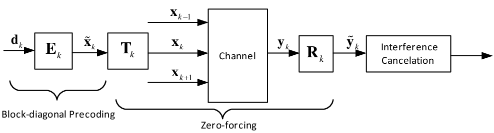
Fig. 7 gives an overview of our proposed achievability scheme, which has a two-layered linear processing structure. The zero forcing achieved by linear transformations and discussed in Section IV constitutes the inner layer, with which an equivalent partially-connected full-rank MIMO-IC is obtained, as shown in Fig. 3 and Fig. 4 for the low- and high-interference cases, respectively. The outer layer of the proposed scheme consists of a block-diagonal precoding matrix at the transmitter and interference cancelation, if necessary, at the receiver. For the high-interference case, is carefully designed so that interference alignment is achieved for the most general cases; whereas for the low-interference case, a random is sufficient since most interfering links are zero forced by the inner layer. In the remaining part of this section, we present the detailed design for the outer precoding matrix for both the low- and high-interference cases. It is worth mentioning that we assume the DoF quantities in the following are all integer values, so that each signaling block is assigned with integer number of symbols. If this is not the case, a spatial extension by an appropriate factor is required, and all the arguments presented in the following still hold in the spatially-extended channel. After DoF normalization by the same factor, the achievability result for the spatially-normalized DoF in Theorem 1 follows.
VI-A Low-Interference Case:
For the low-interference case, the spatially-normalized DoF value is given by
| (48) |
In the following, we will separately consider the two cases when each term in (48) is active.
VI-A1
First, we assume that the rank of the direct channel is sufficiently large so that . In this case, we have , which implies . We show that each user is able to transmit data symbols, denoted as , .
The information-bearing signal vector is decomposed as , and it is precoded with a block-diagonal matrix , which gives
| (49) |
Based on the partition of as shown in Fig. 3, the sizes of , , are given by , , and , respectively, where , and are chosen to satisfy
| (50a) | ||||
| (50b) | ||||
| (50c) | ||||
| (50d) |
With each diagonal block in randomly generated, the conditions given in (VI-A1) ensure that is of full column rank, which is necessary for the full decodability of the desired symbols. It can be verified that with , one feasible choice to satisfy (VI-A1) is
| (51) | ||||
Next, we show that the full decodability condition (47) is satisfied. Due to symmetry, we only need to consider receiver . With zero forcing achieved by and in the inner layer, it is observed from Fig. 3 that receiver only sees the interfering signals and . Therefore, we have
| (52) |
As a result, condition (47) is satisfied with equality; and hence is achievable.
VI-A2
In this case, we have . Then the DoF value per user can be achieved by reducing the number of data streams of any information sub-blocks given in (51), till we have .
VI-B High-Interference Case:
Similar to the low-interference case, the information-bearing signal for the high-interference case is decomposed as and it is precoded with a block-diagonal matrix as shown in (49). The sizes of , and are now given by , , and , respectively, which correspond to the partition of as in Fig. 4. To ensure the decodability of desired data symbols at each receiver, the number of symbols , and of each sub-block in are chosen to satisfy
| (53a) | ||||
| (53b) | ||||
| (53c) | ||||
| (53d) |
The blocks and for the head and tail antennas are randomly generated, so that under the conditions given in (VI-B), they are of full column rank almost surely. In the remaining part of this subsection, for different values activated in (3), we present a feasible selection of , and to satisfy (VI-B), as well as the designs of the precoding matrices for the middle antennas so that the full decodability condition given in (47) is satisfied.
Similar to the low-interference case, if the DoF is limited by the direct channel, i.e. , the achievability scheme can be simply obtained by reducing the number of data symbols transmitted for the interfering-link-limited cases. Therefore, in the following, we assume without loss of generality that the rank of the direct channel is large enough, i.e., , so that the achievable DoF is limited by the interfering links. In this case, it can be verified that in (3) for the high-interference case can be further written as
| (54) |
where . In the following, we will separately consider the cases when each term in (54) is active.
VI-B1
VI-B2
In this case, can be further written as
| (56) |
where . It can be verified that a feasible choice to (VI-B) is
| (57) | ||||
| (58) | ||||
| (59) |
With such a symbol assignment for each sub-block of , the total dimension occupied by the interference at receiver can be calculated based on Fig. 4. Since and as defined in (19) and (21) are full-rank square matrices, interference cancelation can be applied, i.e., the interference caused by and can be subtracted out from by appropriate linear processing with and , respectively. Therefore, we have
| (60) |
where and are full column rank matrices given in (20).
Next, the middle precoding matrices , with and given by (58), are carefully designed so that the interference dimension is small enough to ensure the decodability condition (47) is satisfied. To this end, interference alignment is required in general. We will illustrate the main idea with and , and defer the design of for general values to Appendix A.
Case I: . By substituting with , (56) reduces to
| (61) |
In this case, the matrices are randomly generated from . Then we have
| (62) |
Together with (60), we have
| (63) |
which can be verified to be no greater than for both cases in (61). Therefore, the full decodability condition (47) is satisfied; and hence the DoF value given in (61) for is achievable.
First, we consider the case so that the objective is to transmit data symbols for each user. In this case, we need to apply the technique of “subspace alignment chains” introduced in [10] to the middle antennas as shown in Fig. 4 for the design of . Based on (20), the equivalent system where the subspace alignment chains are applied can be written as . As given in [10], with transmit and receive antennas, the length of the alignment chain is equal to , where we have and . Following the notations used in [10], we use , where , to denote the th -dimensional subspace at transmitter that participates in the chain originated from transmitter , where is a design parameter. For the current case considered, we let
| (65) |
We first consider the alignment chain that originates from transmitter , i.e., . With , the chain length is , or equivalently, two subspaces participate the interference alignment for each chain. In this case, the interference alignment must be achieved at receiver , and the alignment chain can be represented as
| (66) |
The alignment condition (66) is achievable by designing the -dimensional matrices and such that
| (67) |
(67) can be equivalently written as
| (68) |
Since is an matrix, the dimension of its null space is , which can be verified to be no smaller than under and . Therefore, the columns of can be chosen to be the basis vectors for the null space of , based on which the matrices and can be obtained.
With a similar approach, we can design the precoding matrices to achieve two other alignment chains that originate from transmitter 2 and 3, which are represented as
| (69) | ||||
| (70) |
Lastly, the precoding matrices for the middle antennas of the three users are given by
| (71) | ||||
With similar arguments as that in [10], it can be shown that the precoding vectors obtained above are linearly independent and hence the resulting is of full column rank. The interference dimension in (60) can be calculated as
| (72) |
where the minus term is due to the interference alignment achieved by two -dimensional subspaces at receiver . Together with (60) and , we have Therefore, the full decodability condition (47) is satisfied with equality; and hence the DoF given in (64) for the case is achievable.
Next, we consider the case in (64) so that the objective is to transmit data symbols for each user. Let be the dimension of the null space of defined in (68). First, the -dimensional precoding matrices are designed similarly to achieve interference alignment given in (66), (69) and (70). Since for each user, two such precoding matrices are used as shown in (71), the number of data symbols participating interference alignment for each user is given by , which is less than as required by (58) under . Therefore, for each user , we need to transmit another data symbols with precoding matrices denoted as , where
Furthermore, are randomly generated. Then the precoding matrices for the middle antennas are obtained as
It can be verified that the resulting is of full column rank. The interference dimension at the middle antennas of receiver is given by
Together with (60), we have
Therefore, the decodability condition (47) is satisfied with equality; and hence is achievable.
VII Numerical Results
In this section, we provide a numerical example for the proposed techniques. We assume that each terminal is equipped with a uniform linear array (ULA) with adjacent elements separated by distance , where is measured in wavelength. The channel matrix between transmitter and receiver can then be modeled as [17]
| (73) |
where represents the number of signal paths; and denote the angle of arrival (AoA) and angle of departure (AoD) for the th path between transmitter and receiver , respectively. Moreover, and are the transmit and receive array response, respectively, which are given by
| (74) | ||||
| (75) |
Since in (73) is given by a summation of rank-1 matrices, it is clear that in the poor scattering environment with , the channel matrix will be rank deficient.
We consider a 3-user MIMO-IC with and , and all direct links have two paths and the interfering links have one single path only . With the AoAs and AoDs randomly generated, this corresponds to a rank-deficient MIMO-IC with and . Based on Theorem 1, the DoF per user is , i.e., each receiver is expected to be able to detect two data streams sent by their respective transmitters. As a numerical illustration, we consider a particular channel realization for a set of randomly generated AoAs and AoDs given by
| (76) |
| (77) |
where the th entry of and represent the AoA and AoD of the first path for the link between transmitter and receiver , respectively, and the th entry of and are the AoA and AoD of the second path for the direct link . With the scheme presented in Section VI, the precoding matrices in Fig. 7 can be any randomly generated diagonal matrices, and can be found as
| (78) | ||||
| (79) |
Furthermore, with the following linear transformation applied at receiver :
| (80) |
it can be verified that the second and the third antennas of only contain the two desired data symbols sent from transmitter , and hence can be used to fully decode the desired symbols. Similarly, receiver and can both detect their desired data symbols after applying and , respectively.
VIII Conclusion
In this paper, we have provided the complete DoF characterization for the spatially-normalized DoF of the -user rank-deficient MIMO-IC parameterized by . By exploiting the rank-deficiency of the interfering channel matrices and applying invertible linear transformations, we first convert the original fully-connected rank-deficient MIMO-IC into an equivalent partially-connected full-rank MIMO-IC, based on which the existing techniques developed for full-rank channels can be incorporated to facilitate the outer and inner bounds derivations. The outer bound is obtained by the genie-aided signaling technique, where the appropriate genie signals to be provided to the receivers are determined based on the developed equivalent channel model. To achieve the optimal DoF, a two-layered linear processing scheme that combines zero forcing, interference alignment and interference cancelation is proposed. Therefore, for rank-deficient MIMO-ICs, zero forcing or interference alignment alone is not sufficient to achieve the optimal DoF; instead, a combination of the two is required in general.
While we have shown the DoF achievability using the technique of spatial extension for non-integer DoF values, whether the outer bound can still be achieved if we restrict to time/frequency extension only remains an open problem. The additional complexity introduced by such a restriction is the resulting block diagonal channel structure, which needs to be handled more carefully. Another open problem is how to extend the techniques developed in this paper to the completely asymmetric rank-deficient scenario. This will be a challenging task since the design of the zero-forcing matrices, for instance, is much more involved due to a considerably larger number of parameters need to be considered.
Appendix A Achievability of
In this section, we show the achievability of in (56) for general .
A-A Achievability of
We first consider the case when so that . Then from (58), we have , which is the number of independent symbols need to be transmitted by each user via the middle antennas with precoding matrix . With subspace alignment chains technique, we use , where , to denote the th -dimensional subspace at transmitter that participates in the chain originated from transmitter . Here, we let .
We first consider the alignment chain that originates from transmitter . With , where and representing the number of transmit and receive antennas in the middle block as shown in Fig. 4, it follows from [10] that the chain length is equal to . Following similar notations used in [10], we let , , , and . Then the alignment chain that originates from transmitter can be represented as
| (81) |
The alignment chain in (81) can be equivalently written as , where
Since is a matrix, the dimension of its null space is given by . With , it can be verified that is always satisfied. Therefore, the linearly independent columns of are chosen from the null space of , from which we can obtain .
Similarly, we can design the precoding matrices for two other -dimensional subspace alignment chains with chain length that originate from transmitter and transmitter , respectively. The precoding matrix for the middle antennas is then given by
Since there are vectors participating in each alignment chain, in total symbols are transmitted from the middle antennas by all the three users. Due to symmetry, each user transmits symbols by the the middle antennas, which is equal to , as desired. Following similar arguments as that in [10], it can be shown that the columns in are linearly independent and is full column rank.
A-B Achievability of
With , we show that each user is able to transmit independent data streams. From (58), the number of symbols need to be transmitted by the middle antennas is given by . To this end, we need to use two groups of alignment chains, one with chain length and subspace dimension , and the other with chain length and subspace dimension . The design of the first group of alignment chains follows exactly the same manner as the previous case, except that now the number of columns of is set to be . The number of symbols transmitted by the first group of alignment chains from the middle antennas is then given by , which is less than under the condition . Therefore, we need to use another group of alignment chains of length . For this group of alignment chains, we use , where , to denote the th -dimensional subspace at transmitter that participates in the chain originated from transmitter . To ensure data symbols sent by the middle antennas, we let
Then the alignment chain originated from transmitter can be represented as
| (82) |
or equivalently
| (83) |
where is a sub-matrix of given by
The size of is and thus the dimension of its null space is given by . Note that since the submatrix of formed by its first rows also satisfy (83). To ensure the linear independence among the precoding vectors, the columns of are selected from the null space of , but not in the subspace spanned by the columns of the aforementioned submatrix of . The dimension is
It can be verified that , therefore, the columns of can be obtained. Similarly, the precoding vectors and for the other two alignment chains originating from transmitter and can be found. The overall precoding matrix for the middle antennas of user is then obtained accordingly. For the two groups of alignment chains discussed above, the number of aligned interference dimensions at each receiver are respectively given by and . Therefore, with the proposed precoder design, we have
| (84) |
Then together with (60), we have . In other words, the full decodability condition (47) is satisfied with equality. Therefore, is achievable.
References
- [1] R. Etkin, D. Tse, and H. Wang, “Gaussian interference channel capacity to within one bit,” IEEE Trans. Inf. Theory, vol. 54, no. 1, pp. 5534–5562, Dec. 2008.
- [2] A. Host-Madsen and A. Nosratinia, “The multiplexing gain of wireless networks,” Int. Symp. on Inf. Theory and Its Applications, pp. 2065–2069, 4-9 Sept. 2005.
- [3] S. A. Jafar and M. Fakhereddin, “Degrees of freedom for the MIMO interference channel,” IEEE Trans. Inf. Theory, vol. 53, no. 7, pp. 2637–2642, Jul. 2007.
- [4] V. R. Cadambe and S. A. Jafar, “Interference alignment and degrees of freedom of the -user interference channel,” IEEE Trans. Inf. Theory, vol. 54, no. 8, pp. 3425–3441, Aug. 2008.
- [5] T. Gou and S. A. Jafar, “Degrees of freedom of the user MIMO interference channel,” IEEE Trans. Inf. Theory, vol. 56, no. 12, pp. 6040–6057, Dec. 2010.
- [6] V. R. Cadambe, S. A. Jafar, and C. Wang, “Interference alignment with asymmetric complex signaling - Settling the Host-Madsen-Nosratinia conjecture,” IEEE Trans. Inf. Theory, vol. 56, no. 9, pp. 4552 – 4565, Sep. 2010.
- [7] S. A. Jafar, Interference Alignment: A New Look at Signal Dimensions in a Communication Network. Foundations and Trends in Communications and Information Theory, 2010, vol. 7, no. 1.
- [8] A. S. Motahari, S. O. Gharan, and A. K. Khandani, “Real interference alignment with real numbers,” ArXiv pre-print at http://arxiv.org/abs/0908.1208, Aug. 2009.
- [9] V. S. Annapureddy, A. E. Gamal, and V. V. Veeravalli, “Degrees of freedom of interference channels with CoMP transmission and reception,” IEEE Trans. Inf. Theory, vol. 58, no. 9, pp. 5740–5760, Sep. 2012.
- [10] C. Wang, T. Gou, and S. A. Jafar, “Subspace alignment chains and the degrees of freedom of the three-user MIMO interference channel,” to appear in IEEE Trans. Inf. Theory, ArXiv pre-print at http://arxiv.org/abs/1109.4350.
- [11] S. H. Chae and S. Y. Chung, “On the degrees of freedom of rank deficient interference channels,” in IEEE International Symposium on Information Theory, 2011, pp. 1367–1371.
- [12] S. R. Krishnamurthy and S. A. Jafar, “Degrees of freedom of 2-user and 3-user rank-deficient MIMO interference channels,” in IEEE Global Telecom. Conf. (GLOBECOM), 2012, pp. 2486–2491.
- [13] S. R. Krishnamurthy, A. Ramakrishnan, and S. A. Jafar, “Degrees of freedom of rank-deficient MIMO interference networks,” available online at http://escholarship.org/uc/item/1c17p6zq.
- [14] S. A. Jafar and S. Shamai, “Degrees of freedom region of the MIMO channel,” IEEE Trans. Inf. Theory, vol. 54, no. 1, pp. 151–170, Jan. 2008.
- [15] E. Telatar, “Capacity of multi-antenna Gaussian channels,” European Trans. Tel., vol. 10, no. 6, pp. 585–596, Nov. 1999.
- [16] K. S. Gomadam, V. R. Cadambe, and S. A. Jafar, “A distributed numerical approach to interference alignment and applications to wireless interference networks,” IEEE Trans. Inf. Theory, vol. 57, no. 6, pp. 3309–3322, Jun 2011.
- [17] R. B. Ertel, P. Cardieri, K. W. Sowerby, T. S. Rappaport, and J. H. Reed, “Overview of spatial channel models for antenna array communication systems,” IEEE Personal Communications, pp. 10–22, Feb. 1998.