Evaluating $L$-functions with few known coefficients

We are concerned with numerically evaluating $L$-functions. The standard tool, which is used in available open-source computational packages [15, 8] is the approximate functional equation. See Proposition 3.1 for the precise formulation.

There are two main difficulties in evaluating high degree $L$-functions. The first is that if the $L$-function $L(s)$ has degree $d$, evaluating $L(\frac{1}{2}+it)$ using the approximate functional equation requires $\gg(1+|t|)^{d/2}$ Dirichlet series coefficients. Here the implied constant depends on the $L$-function and the desired precision in the answer. For example, estimating the implied constant from the calculations in Section 4, to find the first 1 million zeros of $L(s,\Upsilon_{20},\mathrm{adj})$, the degree 10 $L$-function associated to $\Upsilon_{20}$, would require using the approximate functional equation with around $10^{30}$ Dirichlet series coefficients. Note that 1 million zeros is not even a large sample; for example it is probably not sufficient for testing various conjectures about the lower-order terms in the distribution of spacings between zeros.

The second difficulty is that current methods are incapable of producing a large number of Dirichlet coefficients of the standard and adjoint $L$-functions of a Siegel modular form. The Fourier coefficients indexed by quadratic forms with discriminant up to 3000000 have been computed for $\Upsilon_{20}$ [12]. These Fourier coefficients are used to compute the Hecke eigenvalues. Examination of formulas on page 387 of [18] shows that to find the eigenvalue $\lambda(n)$ of $T(n)$, for $n=p^{2}$, requires the Fourier coefficients indexed by quadratic forms of discriminant up to $n^{2}=p^{4}$.

It gets worse. By (2.2) and (2.4), the $p$th Dirichlet coefficient of the standard or adjoint $L$-function requires both $\lambda(p)$ and $\lambda({p^{2}})$. Thus, to determine the first $n$ Dirichlet coefficients of those $L$-functions requires Fourier coefficients of the Siegel modular form of index up to approximately $n^{4}$. The extensive calculations in [12] are not even sufficient to determine the 83rd Dirichlet coefficient of the standard or adjoint $L$-functions of $\Upsilon_{20}$.

Of course, one could determine more Dirichlet coefficients by first finding more Fourier coefficients of the cusp form. But the $n^{4}$ relationship makes this quite expensive, so with current methods it is not feasible to determine many more Dirichlet coefficients than currently known. It is possible that new methods will be developed to determine the Hecke eigenvalues without extensive computation. The real problem will still remain: how to compute high-degree $L$-functions without requiring an enormous number of Dirichlet coefficients.

That brings us to the theme of this paper: how accurately can one compute an $L$-function given a limited number of Dirichlet coefficients. As the above discussion indicates, this is a practical problem and there are many $L$-functions for which it is not currently possible to determine a reasonably large number of Dirichlet coefficients.

As we describe in this paper, even without knowing many Dirichlet coefficients, we were able to evaluate the $L$-functions to surprisingly high accuracy (surprising to us, anyway). In fact, we were not able to establish that there is an absolute limit to the accuracy one can obtain from only a limited number of coefficients. However, our method is computationally expensive – much more expensive than evaluating the $L$-function in a straightforward way if more coefficients were available. If one could find an efficient way to determine the unknown parameters in our method, that could make it possible to quickly evaluate high-degree $L$-functions. See Section 6 for a discussion.

In the next section we describe the $L$-functions we consider here, and in Section 3 we recall the approximate functional equation and how it is used to compute an $L$-function. In Section 4 we state the underlying problem and then describe our experiments evaluating $L(s,\Upsilon_{20},\mathrm{stan})$ and $L(s,\Upsilon_{20},\mathrm{adj})$. In Section 5 we describe a second method that performs a little better than the method in Section 4 and show how this second method can be used to approximate unknown Dirichlet series coefficients.

We thank the referee for suggesting we include the material in Section 4.3.

The material in this section is taken from Section 3.2 of [15].

Let

be a Dirichlet series that converges absolutely in a half plane, $\Re(s)>\sigma_{1}$.

Let

with $Q,\kappa_{j}\in{\mathbb{R}}^{+}$, $\Re(\lambda_{j})\geq 0$, and assume that:

1. 1.

   $\Lambda(s)$ has a meromorphic continuation to all of ${\mathbb{C}}$ with simple poles at $s_{1},\ldots,s_{\ell}$ and corresponding residues $r_{1},\ldots,r_{\ell}$.

2. 2.

   $\Lambda(s)=\varepsilon\overline{\Lambda(1-\overline{s})}$ for some $\varepsilon\in{\mathbb{C}}$, $|\varepsilon|=1$.

3. 3.

   For any $\sigma_{2}\leq\sigma_{3}$, $L(\sigma+it)=O(\exp{t^{A}})$ for some $A>0$, as $\left|t\right|\to\infty$, $\sigma_{2}\leq\sigma\leq\sigma_{3}$, with $A$ and the constant in the ‘Oh’ notation depending on $\sigma_{2}$ and $\sigma_{3}$.

Note that (3.2) expresses the functional equation in more general terms than (2.5), but it is a simple matter to unfold the definition of $\Gamma_{\mathbb{R}}$ and $\Gamma_{\mathbb{C}}$.

To obtain a smoothed approximate functional equation with desirable properties, Rubinstein [15] introduces an auxiliary function. Let $g:\mathbb{C}\to\mathbb{C}$ be an entire function that, for fixed $s$, satisfies

as $\left|\Im{z}\right|\to\infty$, in vertical strips, $-x_{0}\leq\Re{z}\leq x_{0}$. The smoothed approximate functional equation has the following form.

In our examples $L(s)$ continues to an entire function, so the first sum in (3.4) does not appear. For fixed $Q,\kappa,\lambda,\varepsilon$, and sequence $b_{n}$, and $g(s)$ as described below, the right side of (3.4) can be evaluated to high precision.

A reasonable choice for the weight function is

which by Stirling’s formula satisfies (3.3) if $c>0$, or if $c=0$ and $|b|<\pi d/4$, where $d$ is the degree of the $L$-function. Rubinstein [15] uses such a weight function with $b$ chosen to balance the size of the terms in the approximate functional equation, minimizing the loss in precision in the calculation. In this paper we exploit the fact that there are many choices of weight function, and so there are many ways to evaluate the $L$-function. We combine those calculations to extract as much information as possible from the known Dirichlet coefficients. This idea is described in the next section.

In the computations we carry out below, we find it more convenient to use the Hardy $Z$-function in our computations instead of the $L$-function itself. The function $Z$ associated to an $L$-function $L$ is defined by the properties: $Z(\frac{1}{2}+it)$ is a smooth function which is real if $t$ is real, and $|Z(\frac{1}{2}+it)|=|L(\frac{1}{2}+it)|$.

In Figure 1 we see that there are many values of the parameters in the test function which give reasonable results. If there is some degree of independence in the errors, then there is hope for obtaining a smaller error by combining the results of those separate calculations. Write $Z(s,\Upsilon_{20},\mathrm{stan},\beta)$ for the output of the approximate functional equation with weight function $g(s)=e^{-i\beta s}$. Consider

where $\sum c_{\beta_{j}}=1$. We make the specific choices

Recall that all decimal numbers are truncations of the actual values; one requires much higher precision than the displayed numbers in order to obtain the answers below. With the choices in (4.8), after substituting the known Dirichlet coefficients and then using the Ramanujan bound, we find

Thus, by averaging only 5 evaluations of the $L$-function, the error decreased by a factor of almost $10^{-5}$.

The weights $c_{\beta_{j}}$ in (4.8) were determined by finding the least-squares fit to

where $Ram(b_{n})$ is the Ramanujan bound (2.6) for $b_{n}$, subject to $\sum c_{\beta_{j}}=1$. Note that in our actual examples the vast majority of unknown coefficients have prime index, so the $Ram(b_{n})$ weighting is not important, but we include it for completeness. For the calculations in this paper, we use the $n<1000$ for which $b_{n}$ is unknown in (4.10).

The error estimate in (4.9) is an $L^{1}$ estimate, not the $L^{2}$ estimate as shown in (4.10), so actually it is possible to choose slightly better weights than those used in our example. In Section 5 we show how to obtain the optimal result that can arise from combining different evaluations of the $L$-function, but for now we merely wish to illustrate the seemingly surprising fact that appropriately combining several evaluations can vastly decrease the error.

In Figure 3 we plot the error obtained by combining varying numbers of weight functions, where we evaluate $Z(\frac{1}{2}+10i,\Upsilon_{20},\mathrm{stan})$ with a weight function $g(s)=e^{i\beta s}$ with $\beta=j/10$ with $-10\leq j\leq 25$. The horizontal axis is the number of terms averaged, where we start with $\beta=\tfrac{1}{2}$ and first use those $\beta$ which are closest to $\frac{1}{2}$. The vertical axis is the error estimate on a $\log_{10}$ scale. The lowest point on the graph, when we average all 36 evaluations, corresponds to

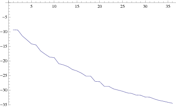
It is not clear from Figure 3 whether one would expect to obtain an arbitrarily small error by combining sufficiently many test functions in the approximate functional equations. This is discussed in Section 6.

We briefly describe the corresponding calculations for $Z(\frac{1}{2}+5i,\Upsilon_{20},\mathrm{adj})$. Recall that, as shown in Figure 2, with a single test function of the standard form we are not able to determine whether that value is positive or negative. Now we combine five evaluations in the analogous way:

where $\sum c_{\beta_{j}}=1$. Here the weight function is $g(s)=e^{-i\beta s+(s-5i)^{2}/500}$.

We make the specific choices

The result is

So we have determined that $Z(\tfrac{1}{2}+5i,\Upsilon_{20},\mathrm{adj})$ is positive, but we can only be certain of one significant figure in its decimal expansion. Using this method, the best result we were able to obtain, by averaging 11 evaluations, is

Averaging more weight function actually makes the result worse. The explanation is simple: since the adjoint $L$-function has high degree, the error terms $\delta_{n}$ decrease very slowly. The least-squares fit does not properly take into account the contribution of a large number of small terms, so the least-squares fit actually has a large $L^{1}$ norm.

In the next section we describe some “sanity checks” on our method, as suggested by the referee. Then, in Section 5, we introduce a different method which avoids some of the shortcomings in the least-squares method.

We check that our method gives correct results in some cases where it is possible to evaluate the $L$-function using another method.

First we consider $L(s,\Delta)$, where $\Delta$ is the (unique) weight 12 cusp form for $SL(2,\mathbb{Z})$, which satisfies the functional equation

We will evaluate $Z(\tfrac{1}{2}+100i,\Delta)$ without using any Dirichlet coefficients, other than the leading coefficient 1. That is, all we know about the $L$-function is its functional equation and the fact that its Dirichlet coefficients satisfy the Ramanujan bound.

In the approximate functional equation we will use the test function $g_{\beta}(s)=e^{-i\beta s+(s-100i)^{2}/100}$, for $\beta=-\frac{30}{20},-\frac{29}{20},...,\frac{69}{20},\frac{70}{20}$. That is a total of 101 evaluations. Using the least-squares method described previously, we find 101 coefficients $c_{\beta}$ with $\sum c_{\beta}=1$. Forming the weighted sum of the 101 evaluations of $Z(\tfrac{1}{2}+100i,\Delta)$ and estimating the unknown terms as described previously, we find

The given digits are correct to the claimed accuracy: the last three digits shown should be 880, and the actual difference between the calculated value and the true value is $9.66\times 10^{-44}$.

Next we consider the $L$-function associated to a weight 24 cusp form for $SL(2,Z)$. Note that $S_{24}(SL(2,\mathbb{Z})$ is two dimensional, and every cusp form $f$ in that vector space satisfies the functional equation

We will attempt to evaluate $Z(\frac{1}{2}+100i,f)$ using as few coefficients as possible. Because there is more than one function satisfying (4.18), it seems obvious that we cannot evaluate such an $L$-function without knowing any coefficients.

If we assume the cusp form $f$ is a Hecke eigenform, then the Dirichlet coefficient $b_{2}$ determines the coefficients $b_{4}$, $b_{8}$, etc, and it also allows us to eliminate every even-index Dirichlet coefficient as an “unknown.” Since that does not seem like an adequately strenuous test of the method, instead we will assume nothing about the Dirichlet series except the functional equation (4.18) and a bound on the Dirichlet coefficients. We will assume a Ramanujan bound of the form $|b_{n}|\leq C_{f}d(n)$, where $d(n)$ is the divisor function and $C_{f}$ is a constant depending only on the cusp form $f$. Is $f$ is a Hecke eigenform then $C_{f}=1$, and if $f=Af_{1}+Bf_{2}$ where $f_{1},f_{2}\in S_{24}(SL(2,\mathbb{Z})$ are the Hecke eigenforms, then $C_{f}=|A|+|B|$.

Using the same 101 test functions as in the case of $L(s,\Delta)$, and choosing 101 weights to minimize the contribution of $b_{3}$, $b_{4}$, …, we find

Thus, we can evaluate $Z(\frac{1}{2}+100i,f)$ to 42 decimal places, knowing (up to a normalizing constant) only one Dirichlet coefficient. The values of $b_{2}$ for the two Hecke eigenforms, in the analytic normalization, are

and inserting those values finds that (4.19) is correct.

Our third check on the method is to evaluate a degree 10 $L$-function which can be also evaluated in an independent way. To give a reasonable match with the case of $L(\frac{1}{2}+5i,\Upsilon_{20},\mathrm{adj})$, we consider $L(\frac{1}{2}+5i,f)^{5}$, where $f$ is a weight 24 cusp forms for $SL(2,\mathbb{Z})$. In other words, the same $L$-function as in the previous example, except that we take its 5th power and evaluate at $\frac{1}{2}+5i$. Note that this time there are two $L$-functions with the given functional equation, with known values:

We will assume that we know the Euler factors up through $p=79$, just as in the case of $L(\frac{1}{2}+5i,\Upsilon_{20},\mathrm{adj})$. If we only use a single test function of the standard form, then the best error we can obtain is comparable to what we found in the previous degree 10 case:

Using the test functions $g_{\beta}(s)=e^{-i\beta s+(s-5i)^{2}/500}$, selecting the 7 values of $\beta$ in the set $\{-\frac{10}{10},-\frac{2}{10},\frac{4}{10},\frac{6}{10},\frac{11}{10},\frac{17}{10},\frac{18}{10},\frac{25}{10}\}$, and using the least-squares method to find suitable weights, we find

Averaging only 7 evaluations decreased the error by a factor of more than 100, and we see that the calculated values are in fact correct. This confirms that our method gives consistent results in cases of comparably complicated $L$-functions for which it is possible to give an independent check on the calculations.

An interesting side-effect of the linear programming approach is that it allows us to obtain information about the unknown coefficients. Instead of treating the value of the $L$-function as the objective, we can use an unknown coefficient as the objective. Note that all the other constraints in the problem are unchanged. Using the same method as described above we find the following coefficients of the standard $L$-function of $\Upsilon_{20}$:

Since the eigenvalues of $\Upsilon_{20}$ are integral and of a known size, if we were to know $b_{83}$ to 35 digits, we would determine it exactly. This is computationally expensive but perhaps not as expensive as if we were to compute more Fourier coefficients of $\Upsilon_{20}$.

These results can be checked once more Fourier coefficients of $\Upsilon_{20}$ are computed. By the $n^{4}$ argument given in in the introduction, computing exact values of $b_{p}$ for $p\leq 97$ will take about twice as much work as it took to compute those for $p\leq 79$.

References

- [1] Anatolij N. Andrianov. Euler products that correspond to Siegel’s modular forms of genus . Uspehi Mat. Nauk, 29(3 (177)):43–110, 1974.
- [2] Anatolij N. Andrianov. Quadratic forms and Hecke operators, volume 286 of Grundlehren der Mathematischen Wissenschaften [Fundamental Principles of Mathematical Sciences]. Springer-Verlag, Berlin, 1987.
- [3] Spencer Bloch and Kazuya Kato. -functions and Tamagawa numbers of motives. In The Grothendieck Festschrift, Vol. I, volume 86 of Progr. Math., pages 333–400. Birkhäuser Boston, Boston, MA, 1990.
- [4] Siegfried Böcherer. Über die Funktionalgleichung automorpher -Funktionen zur Siegelschen Modulgruppe. J. Reine Angew. Math., 362:146–168, 1985.
- [5] Siegfried Böcherer. Bemerkungen über die Dirichletreihen von Koecher und Maaß. (Remarks on the Dirichlet series of Koecher and Maaß). Technical report, Math. Gottingensis, Schriftenr. Sonderforschungsbereichs Geom. Anal. 68, 36 S., 1986.
- [6] J. Brian Conrey, David W. Farmer, Jon P. Keating, Michael O. Rubinstein, and Nina C. Snaith. Integral moments of -functions. PLMS, 91(3):33–104, 2005.
- [7] J. Brian Conrey, David W. Farmer, and Martin R. Zirnbauer. Autocorrelation of ratios of -functions. Commun. Number Theory Phys., 2(3):593–636, 2008.
- [8] Tim Dokchitser. Computing special values of motivic -functions. Experiment. Math., 13(2):137–149, 2004.
- [9] David W. Farmer, Nathan C. Ryan, and Ralf Schmidt. Testing the functional equation of a high-degree Euler product. Pac. J. Math., 253(2):349,366, 2011.
- [10] Jon P. Keating and Nina C. Snaith. Random matrices and -functions. J. Phys. A, 36(12):2859–2881, 2003. Random matrix theory.
- [11] Helmut Klingen. Introductory lectures on Siegel modular forms, volume 20 of Cambridge Studies in Advanced Mathematics. Cambridge University Press, Cambridge, 1990.
- [12] Winfried Kohnen and Michael Kuss. Some numerical computations concerning spinor zeta functions in genus 2 at the central point. Math. Comp., 71(240):1597–1607 (electronic), 2002.
- [13] Pascal Molin. Intégration numérique et calculs de fonctions L. PhD thesis, Institut de Mathématiques de Bordeaux, 2010.
- [14] Ameya Pitale, Abhishek Saha, and Ralf Schmidt. Transfer of Siegel cusp forms of degree 2. Preprint, 2012.
- [15] Michael O. Rubinstein. Computational methods and experiments in analytic number theory. In Recent perspectives in random matrix theory and number theory, volume 322 of London Math. Soc. Lecture Note Ser., pages 425–506. Cambridge Univ. Press, Cambridge, 2005.
- [16] Nathan C. Ryan. Computing the Satake p-parameters of Siegel modular forms. ArXiv Mathematics e-prints, November 2004.
- [17] Nathan C. Ryan and Gonzalo Tornaría. A Böcherer-type conjecture for paramodular forms. Int. J. Number Theory, 7(5):1395–1411, 2011.
- [18] Nils-Peter Skoruppa. Computations of Siegel modular forms of genus two. Math. Comp., 58(197):381–398, 1992.
- [19] Nils-Peter Skoruppa. Data for rational Siegel eigenforms. Personal website, 2010.
- [20] Wolfram Research Inc. Mathematica (Version 8.0), 2010.
David W. Farmer
American Institute of Mathematics
360 Portage Ave
Palo Alto, CA 94306
USA
\affiliationtwoNathan C. Ryan
Department of Mathematics
Bucknell University
Lewisburg, PA 17837