Stochastic receding horizon control of nonlinear stochastic systems with probabilistic state constraints
Abstract
The paper describes a receding horizon control design framework for continuous-time stochastic nonlinear systems subject to probabilistic state constraints. The intention is to derive solutions that are implementable in real-time on currently available mobile processors. The approach consists of decomposing the problem into designing receding horizon reference paths based on the drift component of the system dynamics, and then implementing a stochastic optimal controller to allow the system to stay close and follow the reference path. In some cases, the stochastic optimal controller can be obtained in closed form; in more general cases, pre-computed numerical solutions can be implemented in real-time without the need for on-line computation. The convergence of the closed loop system is established assuming no constraints on control inputs, and simulation results are provided to corroborate the theoretical predictions.
Keywords - stochastic model predictive control, nonlinear systems, exit time, stochastic optimal control, path integral
I Introduction
The behavior of robotic systems can be uncertain due to a variety of reasons, including noise in sensor measurements and environmental effects. Such effects are often represented by stochastic models (for example, ocean waves [2], wind guests [3] and uneven terrain[4]). For nonlinear stochastic systems, existing methods for constrained optimal control are too computationally demanding for real-time implementation. Specifically, no real-time solution exists for continuous-time nonlinear stochastic systems with probabilistic state constraints. A receding horizon formulation partially lifts some of the computational burden associated with the nonlinear stochastic optimal control problem, but current state of the art does not allow real-time implementation on processors at the low-end of the frequency scale. This paper proposes a solution through a stochastic receding horizon formulation that is real-time implementable for nonlinear systems of modest dimension, and comes with probabilistic guarantees of convergence and state constraint satisfaction.
Within a predictive control framework, uncertainty can be accounted for by either approximating sets that bound the system’s trajectories [5, 6, 7, 8, 9, 10, 11] or by stochastic models, with the latter having some specific advantages. In particular, while methods based on set-bounded models may result in over-conservative designs since they plan for the worst case, the use of probabilistic constraints in the methods which are based on stochastic models, on the other hand, allows for less conservatism. In addition, stochastic model-based methods provide some flexibility by allowing one to adjust the probability that problem constraints are violated. These two qualities enable stochastic model-based methods to offer solutions where set-bounded methods may fail.
The structure of the dynamics, whenever it can be exploited, can greatly facilitate the solution of a mpc (mpc) problem. When the stochastic dynamics is linear, one may choose to apply a Kalman filter or its variants and solve an iterative LQG problem [12]. Alternatively, for linear stochastic systems, the optimal control problem under probabilistic constraints is tackled within a chance-constrained model predictive control framework [13, 14, 15, 16, 17, 18, 19, 20]. Chance-constraint formulations are available for linear discrete time systems with Gaussian noise [18, 21, 22, 23, 24, 25, 26, 27, 28, 29, 20].
While methods exist to enable mpc in linear stochastic systems [18, 21, 22, 23, 24, 25, 26, 27, 28, 29, 20], for most nonlinear systems, the stochastic receding horizon optimal control problem can not be solved in real-time. For example, a particle filter implementation of chance-constrained model predictive control is available for linear systems with probabilistic noise [30, 19], and it is in principle applicable to nonlinear systems too. However, the approximate solutions obtained using this method depend on the number of particles, and convergence is achieved after a sufficiently large number of particles is used. Alternative (discrete-time) methods combine a hybrid density filter with dynamic programming [31], the latter being the natural discrete formulation of the optimal control problem. In the hybrid systems literature we find reach-avoid formulations of this problem [32, 33], in which the indicator function of hitting goal or obstacle sets appears in the cost of the optimal control problem (similarly to what is done in this paper). Computational complexity currently limits the application of these methods to systems with up to three states [33], while requirements for real-time implementation are not imposed. Invariably, computational complexity and accuracy issues surface in all discrete-time and space methods, either primarily due to the use of filters, or simply due to the resolution required in the time or state-space domains.
Time and space-discretization may be avoided if the problem is formulated in continuous space and time. Continuous-time solutions to stochastic optimal control problems are available for systems affine in control and with state independent and time invariant control transition matrix, and it is based on path integrals [34]. A path integral is essentially the solution to a hjb (hjb) equation, obtained after the application of a particular transformation [35]. In certain cases, the path integral is computable numerically using Laplace approximations or Monte Carlo sampling. Different applications of path-integral stochastic optimal control have been explored, such as reinforcement learning [36], variable stiffness control (equivalent to automatic tuning of PD gains) [37] and risk sensitive control [38]. The main issue with path integrals is that for most nonlinear systems the solution is computationally demanding and can not be obtained in real-time on existing processors. This limits the application of path integral to real-time receding horizon control on miniature robots.
The main contribution of this paper is to synthesize a real-time design for stochastic (receding horizon) control, following an exit time [39] formulation of the stochastic optimal control problem, instead of one based on path integrals. The proposed formulation yields a time invariant control vector field, which is optimal in terms of actuation utilization. What enables real-time implementation is the fact that the field can be computed off-line and used on-line in a recursive manner. The formulation is based on a combination of deterministic planning with stochastic optimal control, where successive locally optimal stochastic controls are used to steer a system along a deterministic receding horizon reference trajectory, which is conceptually similar to Differential Dynamic Programming [40] and iterative LQG [12]. While such a two-level planning and control strategies has been used successfully in a deterministic setting [41, 42, 43] there is no stochastic analog yet except our own work [1]. Due to the explicit consideration of stochasticity, the proposed method offers almost sure (with probability one) guarantees of collision avoidance and convergence to a desired region, which are elusive in a deterministic setting.
The work presented in this paper is organized in the following way. Section II states the problem formally followed by an intuitive explanation of our approach in section III. Section IV explains a stochastic optimal control design, which is at the heart of our framework. Section V presents the design of the stochastic receding horizon framework and discusses the existence of solutions for our closed loop system. The convergence properties of the resulting stochastic hybrid system are established in Section VI, and the issue of input saturation is brought up. Section VII offers examples of linear and nonlinear systems, presents simulation results for the cases of unbounded and bounded inputs, and discusses computation methods for complex nonlinear stochastic systems. We conclude in Section VIII.
II Problem Statement
Consider an uncertain dynamical system evolving within an open bounded region . Within , there is a closed set which represents forbidden areas (obstacles). In that sense, the system can safely evolve only in the free workspace .
The dynamics of the system is given in the form of a sde (sde)
| (1) |
where is the state, is the drift term, is the matrix of control vector fields, is the control input, and is the diffusion term. Let be an -dimensional Wiener process on the probability space , where is the sample space, is a -algebra on , is the probability measure and is the filtration (i.e. an increasing family of sub--algebras of ) that is right continuous and contains all -null sets.11 1 The justification and the detailed definition for these mathematical constructions can be found in [44].
In a typical stochastic optimal control problem, one has to find a control sequence to steer the dynamics to a desired configuration, while minimizing the cost functional
where the function is the incremental cost, assumed positive definite.
For general nonlinear systems, global analytic solutions to the above stochastic optimization problem are not available. Numerical solutions can be obtained, but depending on the size of the dynamics and the constraints of the problem, the computation cost can be too high for real-time implementation on processors on the lower side of the frequency scale. This limitation motivates us to seek sub-optimal solutions to the above problem by solving the following relaxation instead.
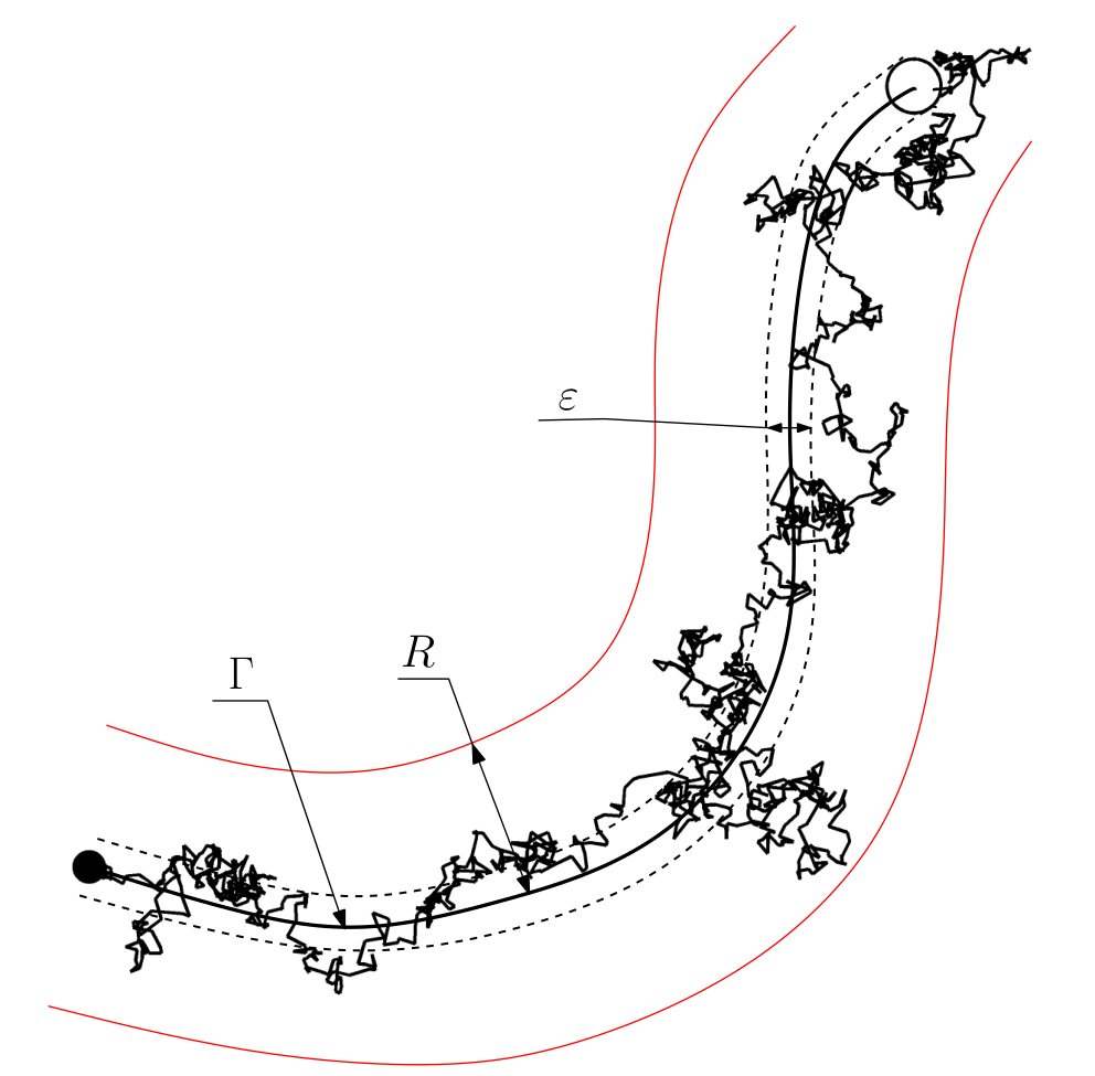
Problem 1 (Modified Problem Statement)
Find a sequence of feedback control laws for (1), such that if is the solution of the system22 2 Assume that the dimension of the controllability distribution is of rank .
| (2) |
for a that minimizes the functional
| (3) | ||||
where, and are positive constants. If denotes the locus (path) of that solution, then for a given selection of points on such that , and , the application of to (1) results in sample paths that achieve
- (i)
(almost-sure safety);
- (ii)
(almost-sure convergence with accuracy );
- (iii)
is minimized, where and are the first times enters an -neighborhood of and , respectively, and is a terminal cost function (local optimality).
Even in this form, the problem does not lend itself to efficiently computed solutions because of the nonlinear infinite-horizon optimal control problem that needs to be solved to obtain . For this reason, the solution of the deterministic optimal control problem will be approximated by the solution of the receding horizon problem
| (4a) | ||||
| (4b) | ||||
where is the prediction horizon of the optimization, function is the same as in (3), and is the terminal cost which approximates the truncated tail of the integral in (3). The idea behind a receding horizon optimization strategy is that one solves the finite horizon optimal control problem and obtains a control law computed for . Control law is applied on (2) for the time interval , , during which time a new control law is computed for , with predicted based on (2). At time , the control law is updated and the process is repeated. It is known [45] that if is a control Lyapunov function for (4b), and
| (5) |
where is a class- function of , then application of results in asymptotically with time. We assume that is a control Lyapunov function for (4b) here as well, and that there exists a positive definite function satisfying (5). In the our modified problem setting, takes the place of and .
III An intuitive example
Consider a robot moving in a two-dimensional space, and described by single integrator dynamics perturbed by stochastic noise:
| (6) |
where is the state vector, is the control input and is a two-dimensional Wiener process. The objective is to find a feedback control law to drive the system -close to the origin, while avoiding the boundary of a circle with radius , centered at the origin.
An obvious control strategy is to just steer the system along a direction toward the origin. A normalized vector pointing to the origin from the current state is . To satisfy the state constraints, the system should be forced away from the circle with radius . One way to achieve this is by weighting the control input by a factor . This results in
| (7) |
It turns out, this intuitive design yields a stochastic control law which is actually optimal. In fact, (7) minimizes the cost
where
and is the first time the state hits either the circle with radius or that with radius . Control law (7) guarantees that the system avoids the -radius circle boundary with probability one, and consequently hits the -radius circle with probability one, because it is known that it almost surely exits the domain somewhere (see [44, Lemma 7.4], and the discussion in the section that follows). Sample paths for the given controller are shown in Fig. 2(a) for different initial conditions.
Assume now that as soon as the system hits the circle of radius around the origin, a coordinate transformation occurs which shifts the origin to a point within distance from its prior location. Then the same controller can be reapplied to drive the system to a -neighborhood of the new origin. An iterative scheme based on this idea can be used to steer the system from point to point in a receding horizon manner. A sample trajectory resulting from an implementation of such a receding horizon controller is shown in Fig. 2(b).
While the design of the controller (7) that enables convergence to way-points is simple for the case of the stochastic single integrator of (6), is not the case for general stochastic nonlinear systems. In following sections, we outline a mathematical framework that allows the computation of receding horizon controllers for more complex stochastic nonlinear systems.
IV Stochastic Optimal Control with Exit Constraints
In this section we design stochastic optimal controllers with exit constraints. These controllers guarantee convergence to a given set, and satisfaction of state constraint, both with probability one. Consider the stochastic system (1)
which evolves within a bounded domain with a boundary and closure denoted . Assume that , , , and are bounded and Lipschitz continuous on . The objective is to find the control that yields
| (8) |
where is the first exit time from the domain . (Notation is standard for .) The incremental cost in (8) is defined as
where . We impose an admissibility condition that there exist a set of control inputs such that for all initial conditions and control inputs , the cost .
The hjb equation associated with (8) is
| (9) |
where the second-order partial differential operator
Equation (9) is written in matrix form as follows
where stands for trace. The optimal control law that solves (9) is then given as
| (10) |
Substituting (10) in (9) yields
| (11) |
Using the logarithmic transformation [35]
and with substitution in (11) we get
| (12) |
with boundary condition
Analytic solutions of the above pde (pde) are generally not possible for complex nonlinear systems. However, the Feynman-Kac formula [44] relates a certain pde with an equivalent sde, and facilitates the numerical solution of the pde through numerical simulation of the sde. Using the Feynman-Kac formula [44], the solution of (12) takes the form
| (13) |
where is the Markov process
| (14) |
evolving on the same bounded open set .
Stochastic Optimal Control with Exit Constraints
Under the assumption
| (15) |
•for some , one can show that , [44, Lemma 7.4]. This means that the system will escape the domain in finite time with probability one. The assumption that and are bounded, ensures satisfaction of (15).
A guarantee that the system does not exit from a specific portion of the boundary can be obtained by imposing an infinite penalty for touching that surface. Consider a partition of the boundary in the form . Then choose as
and
Assuming that and letting , the resulting parabolic pde (12) gives rise to the Dirichlet problem
| (16) | ||||
Then (13) suggests that is in fact the probability that the sample path of (14) from hits boundary before . Function takes the form
| (17) |
and is the Markov process (14). Now if the admissibility condition is satisfied then the optimal control with infinite penalty on exit boundary is equivalent to a constraint (see [39]),
Remark 1
The computation of control input (10) requires , which can be found by either by solving (12) analytically, or numerically simulating (14) and computing (17). As imposes an infinite penalty on state trajectories that exit through , the above construction forces the system to exit through while avoiding with probability one. The problem of stochastic optimal control with terminal cost at exit time is discussed in [35], while a specific problem of exit constraints was discussed in [39]. The latter reference also shows that imposing an exit constraint is equivalent to having infinite penalty on exit location used in this section. We use these two results and thus by defining to be the boundary of state constraint regions, we achieve the guarantees that state constraints are satisfied, and convergence to a desired region is achieved in finite time.
V Stochastic Receding Horizon Control Design
After the presentation of the continuous-time constrained stochastic optimal control formulation in its general setting, we proceed with the description of the implementation of these techniques inside the receding horizon framework that was outlined in the example of Section III. Out of this process emerges a simple, special case of a gshs (gshs), for which the existence of solutions has been established in literature [46]. The section concludes with an examination of the closed loop stability and convergence properties of this simplified gshs, and a discussion on how input saturation affects these properties.
V-A Deterministic Planning
V-B Way-point Generation
Let the closed ball of radius centered at a point is denoted , and its complement, . Now consider a sequence of points with and , satisfying
| (19) |
where is the positive definite function in (5). Define domains , for , such that and
| (20) |
Decompose the boundaries of those domains as follows (see Fig. 3):
| (21) | ||||
| (22) |
The domains are defined such that is non-empty for all .
V-C Stochastic optimal controllers
The system state is a Markov process that evolves between way-points according to the sde
| (23) |
where , , , satisfy the requirements of Section IV, and together with , are all bounded in . The latter is the control input responsible for taking the state from to while avoiding . Let be the first time instant when .
When (23) under hits at some time , it undergoes a forced transition with switching to , and the switch occurs upon the state hitting a part of the boundary . Control law gives a solution to the stochastic optimal control problem
| (24) |
Notice that by setting now the terminal time to allows the value function to be time-invariant. We define the exit time for the process driven by to be . Function is again chosen in a way that it imposes infinite on the state hitting . Similarly to the analysis of Section IV, the solution of (24) is
where , and the optimal control law for is
| (25) |
When applied, satisfies the following probabilistic conditions:
| (26) | ||||
| (27) |
Condition (26) translates into the process exiting in finite time with probability one which is guaranteed by assumption (15). Condition (27) is equivalent to saying that the process reaches an -neighborhood of way-point with probability one, before violating any state constraints (see [39]).
Given a receding horizon path seeded with a sequence of way-points , the process of transitioning from way-point to way-point under (25) is repeated. By the time a new way-point is reached, the path has been recomputed in a receding horizon manner, and the way-point sequence redefined with the initial element being the way-point just reached. What is important for real-time implementation is that for predetermined domains , (25) can be precomputed off-line, numerically in general but also analytically in special cases where , and are such that the boundary value problem for pde (12) can be solved explicitly.
V-D The Resulting Stochastic Hybrid System
Closing the loop around (23) by means of a receding horizon strategy gives rise to a switched stochastic hybrid system, where switching is due to and occurs as a forced transition whenever hits a set . The hybrid state here is just where and are the continuous and discrete states, respectively. This system can be classified as a gshs, a general modeling framework of which is described in [46]; however, it is a very simplified version of the the general definition of [46], which can be adequately described by defining only the following three components: the continuous dynamics, the discrete dynamics, and the reset condition.
Continuous Dynamics
The continuous state evolves according to the sde (23)
| (28) |
where we have just replaced with to emphasize the explicit dependence of the control input on the discrete state , making it a function of the hybrid state : . The drift and diffusion terms, along with , are assumed independent of . When in discrete state , the domain of the continuous variable is .
Discrete Dynamics
The (single) discrete state evolves by means of state-triggered forced transitions, which occur each time the continuous state hits a guard. In this case the guard is a function from to , sending . The time at which the transition is triggered is called stopping time and it is the first time instant . Then the discrete state changes according to the following—in fact, deterministic—rule:
Note that due to the set of discrete states being finite, and the discrete transition map being a bijection, there can only be a finite number of discrete transitions and the system cannot exhibit Zeno behavior.
Reset Condition
During discrete transitions, continuous states are not reset. Essentially, the reset map for the continuous states is simply the identity.
The solution of (28) over , is a collection of Markov processes truncated at (their) exit time, which can be represented as a Markov string. A Markov string is a hybrid state jump Markov process [46]. Given the existence of solutions for each sde (23) for fixed (see [39] for details), and due to the finiteness of the set of discrete states, the solutions for the closed loop stochastic hybrid system are well defined [46].
VI Convergence and Stability Properties
This section presents a proposition that establishes the finite-time convergence properties of the closed loop system to a neighborhood of the origin.
Proposition 1
Consider the switched stochastic system (23) in an open bounded domain , where is the switching index, and is a Wiener process. Let be a , positive definite function in the closure of a bounded domain which contains the origin. If for every solution of the stochastic switched system there exist
- (i)
- (ii)
a class- function on together with a sequence of points satisfying (19),
then the closed-loop switched stochastic system (23)–(25) converges to an -neighborhood of origin in finite time.
Proof:
It is known [45] that a receding horizon strategy applied on (4) yields a trajectory satisfying . Hence, with sufficiently large , one can find a path such that . Moreover, condition (5) ensures that for any , the system will remain within an open bounded set containing the level set of . This means that for a sufficiently large , the path intersects an -neighborhood of the origin and remains bounded. Given that this set is bounded, one can only cover it with a finite number of non-overlapping balls with radius . Hence, for sufficiently large , there is a finite number of way-points that satisfy condition (19) with at the origin. Then, by induction it is shown in a straightforward way that the system reaches an -neighborhood of the origin in finite time.
To this end, set , construct a path of finite length according to (4), and select a way-point according to (19). Given that bounded domain satisfies (20)–(22), the application of control law (25) ensures that for all , , that is, the state at time is in almost surely (see Section IV and [39]). Condition (15) ensures that the time that this happens is finite.
VI-A Convergence under bounded inputs
The control law may require large inputs near the boundary , since there. This can be problematic from an implementation standpoint. When these inputs saturate at some , the control law that is practically implemented is rather approximated smoothly by
The problem is that bounded inputs cannot force exit at with probability one. The probability of success in exiting when bounded inputs are applied can be computed [51], but there there is always a nonzero probability that the system will exit from instead of . Neither convergence to origin nor constraint satisfaction can be guaranteed almost surely.
To recover convergence under bounded inputs, we propose a recovery strategy that uses repeatedly a controller precomputed offline, which steers the system back inside the domain . The receding horizon control can be re-initiated after the state is re-enters . This recovery controller is not different from (25), and its use is illustrated in an example in Section VII. In the absence of obstacles, and with infinitely large outer domain, the guarantee of convergence can thus be recovered even with bounded inputs.
VII Examples
We present two different examples to demonstrate application of our control design. In the first example the stochastic optimal control law can be computed explicitly, and simulation results are presented to demonstrate its function. The effect of input saturation is also investigated. The second example involves a nonlinear system, where the stochastic optimal control laws can not be computed explicitly. There, we show how the application of the Feynman-Kac formula offers numerical controller designs, and we present the results through representative plots.
VII-A The Stochastic Single Integrator
Problem formulation
Consider the system (23) with the drift term and is identity. This simple drift-less system can be described as a two-dimensional single integrator with stochastic uncertainty as
| (29) |
where is the state and is a 2-dimensional Wiener process. The objective is to find control inputs to drive the system to origin, using minimal inputs, avoiding obstacles, and moving along paths of minimal length to its destination. Here the system’s workspace is a ball of radius , containing spherical obstacles with radii and centers , .
Deterministic Path Planning
The first step is to find a reference trajectory for (29) ignoring noise. The nominal dynamics is just . We use the approach of [47] (other methods are also possible) to find a continuous trajectory minimizing a finite-horizon cost
where is the prediction horizon and and are arbitrary positive constants. The terminal cost is selected as a navigation function [52] defined as
| (30) |
where is a sufficiently large positive integer. In (30), the function encodes the location and size of obstacles and is expressed as
with and , for .
Assume that the outcome of this procedure is an obstacle-free continuous state trajectory , and the resulting path is
Way-point Generation
There exist control way-points , such that , and . Define the sets and denote their boundary . The waypoints we select are chosen to satisfy the following constraint:
| (31) | ||||
| (32) | ||||
| (33) |
where and are positive constants. The above constraints also help determine the radius , which is the outer radius of the domain of the continuous state . There is no unique solution for and one can specify an upper and lower bounds on .
Stochastic optimal controller
The control input for (29) is constructed as shown in Section IV. It achieves
where
The optimal control law is
where , , and is the solution of the pde
Function has an analytic expression:
which suggests a value function
and a control law of the form
| (34) |
Control input switches to upon hitting the boundary for until the state is in -neighborhood of the goal.
Problem instantiation and simulation results
Simulations were performed (taking ) with the overall bounded domain being . The initial condition is . The goal is to drive the system to the origin. The workspace contains two obstacles of radius at coordinates and . Matrix is the identity, and is chosen to satisfy and with . A navigation function is constructed on and a trajectory for is generated based on [47]. The simulation of the complete algorithm is shown in the Fig. 4. The navigation function is depicted in the form of a contour plot, while the discrete way-points are center of filled (red) circles. The boundaries are chosen based on (38)– (33) and are marked in the figure by dotted black circles.
The effect of input saturation
The following controller is a saturated version of (34):
| (35) |
Figure 5 shows a sample path for the bounded input case, and quantifies the norm of the inputs used.

As discussed earlier, bounded inputs (35) will not result in success with probability one (i.e. the probability of first hitting ) and the probability of success for each local controller can be computed according to [51]. Figure 6 represents the probability of hitting the goal boundary , before exiting the domain elsewhere for any given initial condition. It can be seen that there is always a nonzero probability that the system exits from instead of under bounded inputs, and this probability becomes higher for initial conditions closer to .
To recover convergence under bounded inputs, we implement the recovery strategy. The implementation is shown in Fig. 7. We observe that the probability of convergence with recovery strategy can be one in absence of obstacles and sufficiently (infinitely) large outer boundary. In the presence of obstacles, the computation of the probability of convergence can only be approximated by a numerical estimation for finite way-points.33 3 The probability of convergence can be shown to be equal to one if we consider the state constraints to be reflective boundary; this is a topic for a different paper.
VII-B A Nonlinear System
Finding a solution to the pde (16) is central to the proposed control design. In Section VII-A, such a solution can be obtained explicitly, but with (16) having varying coefficients, this is not true in general. In this section we demonstrate a solution approach that is based on the Feynman-Kac formula.
Problem formulation
Consider a mobile robot with three omni-directional wheels (Fig. 8). In Fig. 8, , mark the position, with respect an inertial – frame, of the local, body-fixed frame –. The orientation of the local frame with respect to – is given by angle . The dynamical system modeling the robot has as state the vector . The input to the system is a vector of the linear velocities of the three wheels, denoted , , , respectively. Stochastic noise affects all three coordinates , and . The equations of motion for such a system can be represented by the following sde
| (36) |
Remark 2
The goal is to a find control law to drive (36) to the origin , using inputs of minimal magnitude, following paths of minimal length, and avoiding obstacles along the way. The robot’s workspace is a torus, containing a finite number of torus-shaped obstacles at locations , . The robot’s outer workspace boundary, and those of the obstacles for are is defined as
| (37a) | ||||
| (37b) | ||||
Deterministic Path Planning
Using the metric introduces in Remark 2, and the definition of obstacle and outer boundary in (37), we apply the path planning approach of Section VII-A, selecting a fixed satisfying .
Let us denote the obstacle-free continuous state trajectory found using, say [47]. Then the path is expressed directly as .
Way-point Generation
Here we will select a sequence , of waypoints. The objective of stochastic controller for each discrete state is to make (36) converge close to way-point .
To this end, define a set and denote its boundary . Then define domains , and select an arbitrary set of points from , such that , , and for ,
| (38) | ||||
| (39) |
The boundaries and are defined as and , respectively for all .
Stochastic optimal controller
Equation (40) does not admit analytic solutions. Common applicable numerical methods such as finite differences and finite elements have difficulty producing acceptable solutions for instances of problems with dimension larger than three and complex boundary conditions. Alternatively, the Feynman-Kac’s formula (see Section IV), relates the pde to an sde:
| (41) |
which is essentially the unforced system (36). Then, we know that the function satisfies
| (42) |
where is the first exit time from the domain .
Problem instantiation and simulation results
The probability in (42) can be estimated numerically44 4 The source code to compute function is available at http://code.google.com/p/stochastic-receding-horizon-control/ by simulating sufficiently many sample paths of (41) with different initial conditions . We produce these sample paths using the Euler-Maruyama method [53]. Using the same method, we also obtain sample paths for (36). A grid is imposed on the state space, and treating each node as an initial condition, we produce 500 sample paths and estimate (42). With the estimate of (42), the control law is computed numerically as
Figure 9 presents two numerical approximations of in the form of 2D colormaps with robot orientation set at and radians, respectively. Equipped with such a map, a numerical gradient can be used to calculate the control input. Figure 10 shows a single sample path for the closed loop version of (36). The time history of individual states , and are shown in Figs. 11(a)–11(c), indicating the convergence to an neighborhood of the origin. Figure 11(d) plots the norm of the control inputs used. Numerical data confirmed that the probability that the closed loop system hits every desired goal boundary is one.
VIII Conclusions
The proposed method allows the design of a receding horizon navigation controller for nonlinear systems governed by stochastic differential equations. If a feasible path, optimal or otherwise, is available in the form of a finite sequence of way-points, then an an optimal control law can be found to steer the stochastic system between these way-points, while keeping it close to the path and away from unsafe regions with probability one. In cases where control inputs are forced within upper and lower bounds, and state constraints (obstacles) are imposed, almost-sure convergence and safety is impossible, but it can be achieved with some probability which depends on how severe the input bounds are compared with respect to the magnitude of subjected noise. For nonlinear systems with dynamics not permitting analytic solutions for the resulting pdes, numerical solutions for dimensions up to or are shown to be well within the reach of currently available computing platforms.
References
- [1] S. Shah, C. Pahlajani, N. Lacock, and H. Tanner, “Stochastic receding horizon control for robots with probabilistic state constraints,” in Proceedings of the IEEE International Conference on Robotics and Automation, 2012, pp. 2893–2898.
- [2] M. Ochi, Ocean Waves: The Stochastic Approach, ser. Cambridge Ocean Technology. Cambridge University Press, 2005.
- [3] N. Barr, D. Gangsaas, and D. Schaeffer, “Wind models for flight simulator certification of landing and approach guidance and control systems,” U.S. Dept. of Transportation, Tech. Rep., 1974.
- [4] G. Ishigami, G. Kewlani, and K. Iagnemma, “Statistical mobility prediction for planetary surface exploration rovers in uncertain terrain,” in Proceedings of the IEEE International Conference on Robotics and Automation, 2010, pp. 588–593.
- [5] D. Ramirez, T. Alamo, and E. Camacho, “Efficient implementation of constrained min-max model predictive control with bounded uncertainties,” in Proceedings of the 41st IEEE Conference on Decision and Control, vol. 3, 2002, pp. 3168 – 3173.
- [6] D. Ramírez, T. Alamo, E. Camacho, and D. M. de la Peña, “Min-max mpc based on a computationally efficient upper bound of the worst case cost,” Journal of Process Control, vol. 16, no. 5, pp. 511 – 519, 2006.
- [7] D. DeHaan and M. Guay, Model Predictive Control, T. Zheng, Ed. Sciyo, 2010.
- [8] J. M. Carson III, “Robust model predictive control with a reactive safety mode.” Ph.D. dissertation, California Institute of Technology, 2008.
- [9] D. Marruedo, T. Alamo, and E. Camacho, “Input-to-state stable mpc for constrained discrete-time nonlinear systems with bounded additive uncertainties,” in Proceedings of the 41st IEEE Conference on Decision and Control 2002, vol. 4, 2002, pp. 4619 – 4624 vol.4.
- [10] A. A. Jalali and V. Nadimi, “A survey on robust model predictive control from 1999-2006,” in Proceedings of the International Conference on Computational Inteligence for Modelling Control and Automation, and International Conference on Intelligent Agents Web Technologies and International Commerce. Washington, DC, USA: IEEE Computer Society, 2006, pp. 207–212.
- [11] A. Bemporad and M. Morari, “Robust model predictive control: A survey,” in Robustness in identification and control, ser. Lecture Notes in Control and Information Sciences, A. Garulli and A. Tesi, Eds. Springer Berlin / Heidelberg, 1999, vol. 245, pp. 207–226.
- [12] E. Todorov and W. Li, “A generalized iterative lqg method for locally-optimal feedback control of constrained nonlinear stochastic systems,” in Proceedings of the American Control Conference, 2005, pp. 300–306.
- [13] D. Chatterjee, P. Hokayem, and J. Lygeros, “Stochastic receding horizon control with bounded control inputs: A vector space approach,” IEEE Transactions on Automatic Control, vol. 56, no. 11, pp. 2704 –2710, 2011.
- [14] D. Chatterjee, E. Cinquemani, and J. Lygeros, “Maximizing the probability of attaining a target prior to extinction,” Nonlinear Analysis: Hybrid Systems, vol. In Press, Corrected Proof, 2011.
- [15] P. Hokayem, E. Cinquemani, D. Chatterjee, F. Ramponi, and J. Lygeros, “Stochastic receding horizon control with output feedback and bounded controls,” Automatica, vol. 48, no. 1, pp. 77 – 88, 2012.
- [16] A. T. Schwarm and M. Nikolaou, “Chance-constrained model predictive control,” American Institute of Chemical Engineers Journal, vol. 45, no. 8, pp. 1743–1752, 1999.
- [17] P. Li, M. Wendt, and G. Wozny, “Robust model predictive control under chance constraints,” Computers & Chemical Engineering, vol. 24, no. 2-7, pp. 829–834, 2000.
- [18] E. Cinquemani, M. Agarwal, D. Chatterjee, and J. Lygeros, “Convexity and convex approximations of discrete-time stochastic control problems with constraints,” Automatica, vol. 47, no. 9, pp. 2082 – 2087, 2011.
- [19] L. Blackmore, M. Ono, A. Bektassov, and B. Williams, “A probabilistic particle-control approximation of chance-constrained stochastic predictive control,” IEEE Transactions on Robotics, vol. 26, no. 3, pp. 502 –517, 2010.
- [20] L. Blackmore, M. Ono, and B. Williams, “Chance-constrained optimal path planning with obstacles,” IEEE Transactions on Robotics, vol. 27, no. 6, pp. 1080 –1094, 2011.
- [21] M. Cannon, P. Couchman, and B. Kouvaritakis, “Mpc for stochastic systems,” in Assessment and Future Directions of Nonlinear Model Predictive Control, ser. Lecture Notes in Control and Information Sciences, R. Findeisen, F. Allgöwer, and L. Biegler, Eds. Springer Berlin / Heidelberg, 2007, vol. 358, pp. 255–268.
- [22] M. Cannon, D. Ng, and B. Kouvaritakis, “Successive linearization nmpc for a class of stochastic nonlinear systems,” in Nonlinear Model Predictive Control, ser. Lecture Notes in Control and Information Sciences, L. Magni, D. Raimondo, and F. Allgöwer, Eds. Springer Berlin / Heidelberg, 2009, vol. 384, pp. 249–262.
- [23] M. Cannon, B. Kouvaritakis, S. Rakovi and, and Q. Cheng, “Stochastic tubes in model predictive control with probabilistic constraints,” IEEE Transactions on Automatic Control, vol. 56, no. 1, pp. 194 –200, 2011.
- [24] M. Shin and J. A. Primbs, “A riccati based interior point algorithm for the computation in constrained stochastic mpc,” IEEE Transactions on Automatic Control, vol. 57, no. 3, pp. 760 –765, 2012.
- [25] M. Shin and J. Primbs, “A fast algorithm for stochastic model predictive control with probabilistic constraints,” in American Control Conference, 2010, pp. 5489–5494.
- [26] J. Primbs and C. H. Sung, “Stochastic receding horizon control of constrained linear systems with state and control multiplicative noise,” IEEE Transactions on Automatic Control, vol. 54, no. 2, pp. 221 –230, 2009.
- [27] A. T. Schwarm and M. Nikolaou, “Chance-constrained model predictive control,” American Institute of Chemical Engineers (AIChE) Journal, vol. 45, no. 8, pp. 1743–1752, 1999.
- [28] D. van Hessem and O. Bosgra, “A full solution to the constrained stochastic closed-loop mpc problem via state and innovations feedback and its receding horizon implementation,” in Proceedings of 42nd IEEE Conference on Decision and Control, vol. 1, 2003, pp. 929 – 934 Vol.1.
- [29] D. van Hessem, Stochastic Inequality Constrained Closed-loop Model Predictive Control: With Application To Chemical Process Operation. Delft University Press, 2004.
- [30] L. Blackmore, “A probabilistic particle control approach to optimal, robust predictive control,” in In Proceedings of the AIAA Guidance, Navigation and Control Conference, 2006.
- [31] F. Weissel, M. Huber, and U. Hanebeck, “A nonlinear model predictive control framework approximating noise corrupted systems with hybrid transition densities,” in 46th IEEE Conference on Decision and Control, 2007, pp. 3661 –3666.
- [32] S. Summers, M. Kamgarpour, C. J. Tomlin, and J. Lygeros, “A Stochastic Reach-Avoid Problem with Random Obstacles,” in Hybrid Systems: Computation and Control. ACM, 2011, pp. 251–260.
- [33] S. Summers and J. Lygeros, “Verification of discrete time stochastic hybrid systems: A stochastic reach-avoid decision problem,” Automatica, vol. 46, no. 12, pp. 1951 – 1961, 2010.
- [34] H. J. Kappen, “Path integrals and symmetry breaking for optimal control theory,” Journal of Statistical Mechanics: Theory and Experiment, vol. 2005, no. 11, p. P11011, 2005.
- [35] W. H. Fleming, “Exit probabilities and optimal stochastic control,” Applied Mathematics and Optimization, vol. 4, pp. 329–346, 1977.
- [36] E. Theodorou, F. Stulp, J. Buchli, and S. Schaal, “Iterative path integral stochastic optimal control for learning robotic tasks,” in The 18th World Congress of The International Federation of Automatic Control, Milan, Italy, 2011.
- [37] J. Buchli, F. Stulp, E. Theodorou, and S. Schaal, “Learning variable impedance control,” The International Journal of Robotics Research, vol. 30, no. 7, pp. 820–833, 2011.
- [38] B. van den Broek, W. Wiegerinck, and B. Kappen, “Stochastic optimal control of state constrained systems,” International Journal of Control, vol. 84, no. 3, pp. 597–615, 2011.
- [39] M. Day, “On a stochastic control problem with exit constraints,” Applied Mathematics and Optimization, vol. 6, pp. 181–188, 1980.
- [40] D. Jacobson and D. Mayne, Differential dynamic programming, ser. Modern analytic and computational methods in science and mathematics. American Elsevier Pub. Co., 1970.
- [41] R. Burridge, A. Rizzi, and D. Koditschek, “Sequential composition of dynamically dexterous robot behaviors,” The International Journal of Robotics Research, vol. 18, pp. 534–555, 1999.
- [42] F. Lamiraux and J.-P. Laumond, “Smooth motion planning for car-like vehicles,” Proceedings of the IEEE Transactions on Robotics and Automation, vol. 17, no. 4, pp. 498–502, 2001.
- [43] K. Pathak and S. Agrawal, “An integrated path-planning and control approach for nonholonomic unicycles using switched local potentials,” IEEE Transactions on Robotics, vol. 21, no. 6, pp. 1201 – 1208, 2005.
- [44] I. Karatzas and S. E. Shreve, Brownian Motion and Stochastic Calculus, 2nd ed., ser. Graduate Texts in Mathematics. Springer, 1991.
- [45] A. Jadbabaie, “Receding horizon control of nonlinear systems: a control lyapunov function approach.” Ph.D. dissertation, California Institute of Technology, 2001.
- [46] M. Bujorianu and J. Lygeros, “Toward a general theory of stochastic hybrid systems,” in Stochastic Hybrid Systems: Theory and Safety Critical Applications, ser. Lecture Notes in Control and Information Sciences (LNCIS), 2006, vol. 337, pp. 3–30.
- [47] H. Tanner and J. Piovesan, “Randomized receding horizon navigation,” IEEE Transactions on Automatic Control, vol. 55, no. 11, pp. 2640 –2644, 2010.
- [48] E. Rimon and D. Koditschek, “Exact robot navigation using artificial potential functions,” IEEE Transactions on Robotics and Automation, vol. 8, no. 5, pp. 501–518, 1992.
- [49] S. M. Lavalle, J. J. Kuffner, and Jr., “Rapidly-exploring random trees: Progress and prospects,” in Algorithmic and Computational Robotics: New Directions, 2000, pp. 293–308.
- [50] S. M. LaValle, Planning Algorithms. Cambridge, U.K.: Cambridge University Press, 2006.
- [51] S. Shah, C. Pahlajani, and H. Tanner, “Probability of success in stochastic robot navigation with state feedback,” in Proceedings of the IEEE/RSJ International Conference on Intelligent Robots and Systems, 2011, pp. 3911–3916.
- [52] D. E. Koditschek and E. Rimon, “Robot navigation functions on manifolds with boundary,” Advances in Applied Mathematics, vol. 11, no. 4, pp. 412–442, 1990.
- [53] D. J. Higham, “An algorithmic introduction to numerical simulation of stochastic differential equations,” SIAM Review, vol. 43, no. 3, pp. 525–546, 2001.