Distribution rules of crystallographic systematic absences on the Conway topograph and their application to powder auto-indexingThanks: This research was partly supported by a Grant-in-Aid for Young Scientists (B) (No. 22740077) and the Ibaraki prefecture (J-PARC-23D06).

Lattice determination problems have been the target of much interest in mathematics. In particular, many mathematicians worked on lattice determination from a theta series in the second half of the 20th century, with the aim of providing higher dimensional counterexamples for the isospectral problem proposed by Kac [16]. Lattice determination from a theta series was finally resolved in [24], [25]. However, it is not well known in the mathematics community that a similar problem was being studied in crystallography during this period.

The lattice determination problem in crystallography is called powder auto-indexing. There a set of lattice parameters is determined from a powder diffraction pattern. Powder auto-indexing is equivalent to lattice determination from an average theta series, as shown in Appendix A. At present, powder diffraction is the principal technique for determining the structure of materials that do not necessarily form large-sized crystals. A highly automated system of analyzing powder diffraction patterns is required, both for basic scientific research and a wide range of industrial applications, not least in the pharmaceutical industry. Hence, it is necessary to establish a powerful and reliable powder auto-indexing algorithm and software.

In this paper, the powder auto-indexing problem is formulated and solved. This is regarded as a new application of the reduction theory of positive-definite quadratic forms to crystallography. In consideration of its application to crystallography, we mainly discuss cases when the lattice has a rank of $N=2,3$. Similar to a theta series, information about the lengths of lattice vectors is extracted from an average theta series (Section 2). The most notable difference is that it is very difficult to acquire the multiplicities of the lengths (i.e., number of lattice vectors satisfying ${\left\lvert l\right\rvert}^{2}=q$ for fixed $q\in{\mathbb{R}}_{>0}$) from an average theta series, and only a part of the lengths can be obtained owing to the crystallographic phenomenon of systematic absences.

Systematic absences have not been defined sufficiently explicitly as a mathematical notion. We provide a definition in Section 4. As in the International Tables [14], systematic absences are classified by the pair $(G,H)$:

• •

  isomorphism class of the crystallographic group $G\subset O(N)\ltimes{\mathbb{R}}^{N}$,

• •

  conjugate class of the finite subgroup $H\subset G$.

For fixed $N$, systematic absences are categorized by finitely many pairs (Proposition 4.1). When a periodic function $\wp$ belongs to the type $(G,H)$, the lengths of $l^{*}\in\Gamma_{ext}(G,H)$ is not directly extracted from the average theta series of $\wp$, where $\Gamma_{ext}(G,H)$ is a subset of the reciprocal lattice $L^{*}$ of $L$ determined from $(G,H)$.

To date, powder auto-indexing algorithms have been studied and improved by experts in crystallography. Among existing software packages, Ito [10], [29], TREOR (trial-and-error method [34]), and DICVOL (dichotomy method [4]) are widely used. McMaille (a grid search based on the Monte Carlo method [18]) and X-cell (dichotomy method [20]) were developed comparatively recently. With regard to existing powder auto-indexing software, several considerable problems have been reported. These include:

• •

  existence of more than one solutions,

• •

  systematic absences,

• •

  missing or false elements in the set of extracted lengths,

• •

  observation errors contained in the length values,

• •

  large zero-point shift,

• •

  overlapping peaks.

In some software, these problems are caused by limitations intended to suppress the computation time. Therefore, both computation time and success rate should be considered to discuss powder auto-indexing algorithms. (For example, although the simplest brute force grid search may obtain the highest success rate, it takes from a few hours to a few days in monoclinic and triclinic cases.) This paper presents a method that can resolve each of the problems listed above. The first three are explained in more detail in the following discussion. The next two are resolved using the estimated error ${\rm Err}[{\left\lvert l\right\rvert}^{2}]$ of ${\left\lvert l\right\rvert}^{2}$ (see ($A$2) in Section 3 and the beginning of Section 7). The final problem is also resolved naturally in our algorithm (Section 7.4).

Our three main results are as follows. First, we formulate powder auto-indexing as a mathematical problem, and summarize mathematical results on the cardinality of solutions in powder auto-indexing. This is considered the most important foundation for the following discussion; in general, a lattice $L$ is not determined uniquely in $N\geq 2$, even if the rank $N$ of $L$ and all the lengths $l\in L$ are given (Appendix B). On the other hand, the cardinality of $L_{2}$ satisfying $\Lambda_{L}=\Lambda_{L_{2}}$ is always finite in $N\leq 4$, therefore it is possible to enumerate all such $L_{2}$ algorithmically (Appendix C). However, it is not certain whether the number of solutions is actually finite in powder auto-indexing, owing to systematic absences and the finite observational range. Fortunately, using both physical constraints and mathematical theorems, we obtain a necessary condition for assuming the finiteness of solutions, except for events with zero probability (Section 3). As a result, it is only necessary to enumerate finitely many solutions for powder auto-indexing.

Our second result is a new algorithm to enumerate powder auto-indexing solutions (Sections 7.1 and 7.2). We prove that it works regardless of the type of systematic absences. Our basic idea is to use the graph whose edges are associated with a set of squares of lengths ${\left\lvert l_{1}^{*}\right\rvert}^{2}$, ${\left\lvert l_{2}^{*}\right\rvert}^{2}$, ${\left\lvert l_{1}^{*}+l_{2}^{*}\right\rvert}$, ${\left\lvert l_{1}^{*}-l_{2}^{*}\right\rvert}^{2}$ for some lattice vectors $l_{1}^{*},l_{2}^{*}\in L^{*}$.

In Ito’s method, the parallelogram law $2({\left\lvert l_{1}^{*}\right\rvert}^{2}+{\left\lvert l_{2}^{*}\right\rvert}^{2})={\left\lvert l_{1}^{*}+l_{2}^{*}\right\rvert}^{2}+{\left\lvert l_{1}^{*}-l_{2}^{*}\right\rvert}^{2}$ is used to obtain Gram matrices of sublattices of rank 2 (called zones). However, simple use of the parallelogram law does not always provide successful results, as introduced in Fact 1 of Section 6.2. Therefore, instead of just enumerating a set of lengths satisfying the parallelogram law, our algorithm utilizes graphs whose edges are associated with ${\left\lvert l_{1}^{*}\right\rvert}^{2}$, ${\left\lvert l_{2}^{*}\right\rvert}^{2}$, ${\left\lvert l_{1}^{*}+l_{2}^{*}\right\rvert}$, and ${\left\lvert l_{1}^{*}-l_{2}^{*}\right\rvert}^{2}$ as a network of lattice vector lengths. This provides a comprehensive method of analyzing how the two sets $\{{\left\lvert l_{1}^{*}\right\rvert}^{2},{\left\lvert l_{2}^{*}\right\rvert}^{2},{\left\lvert l_{1}^{*}+l_{2}^{*}\right\rvert}^{2},{\left\lvert l_{1}^{*}-l_{2}^{*}\right\rvert}^{2}\}$ and $\{{\left\lvert k_{1}^{*}\right\rvert}^{2},{\left\lvert k_{2}^{*}\right\rvert}^{2},{\left\lvert k_{1}^{*}+k_{2}^{*}\right\rvert}^{2},{\left\lvert k_{1}^{*}-k_{2}^{*}\right\rvert}^{2}\}$ are related to each other.

For lattices of rank 2, such a graph has already been defined by Conway, who called it a topograph [6]. As explained in section 5.1, a graph having the required property is constructed for general $N$ by using Voronoi’s second reduction theory. We also call this a topograph. Basic properties of topographs for lattices of rank $N=2,3$ are explained in Section 5.2.

In Section 6, we shall see how primitive vectors of $l^{*}\in L^{*}$ belonging to $\Gamma_{ext}(G,H)$ are distributed on a topograph. Although the following theorem for the case of $N=2$ has not been described explicitly, it provides a theoretical reason for the parallelogram law working appropriately for $N=2$.

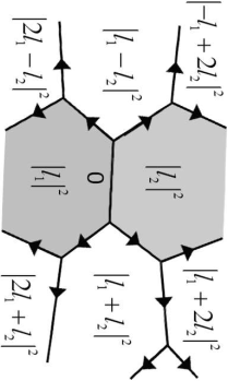
In brief, Theorem 1 claims that $l^{*}\in\Gamma_{ext}(G,H)$ only appear in the gray area in Figure 1, regardless of the type $(G,H)$. With regard to the case of $H=\{1\}$, we shall introduce a proof using topographs in Section 6.1. The case $H\supsetneq L$ is not proved here since it is verified easily by checking lists in [14].

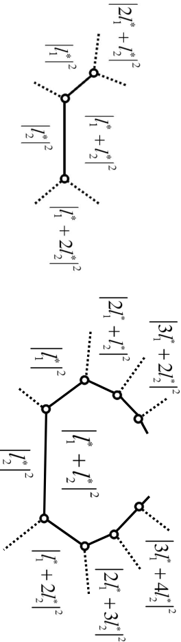
By Theorem 1, a subgraph of a topograph with infinitely many edges is formed by unifying substructures as in Figure 2 associated with the lengths ${\left\lvert l_{1}^{*}\right\rvert}^{2},{\left\lvert l_{2}^{*}\right\rvert}^{2},{\left\lvert l_{1}^{*}+l_{2}^{*}\right\rvert}^{2},{\left\lvert l_{1}^{*}-l_{2}^{*}\right\rvert}^{2}$ of $l_{1}^{*},l_{2}^{*}\in L^{*}\setminus\Gamma_{ext}(G,H)$ that are easily extracted from an average theta series.

For $N=3$, similar statements are proved in Theorems 2 and 3. In this case, it is necessary to use the following formula instead of the parallelogram law:

As another consequence of Theorems 2 and 3, our algorithm enumerates the Gram matrices $(l_{i}^{*}\cdot l_{j}^{*})_{1\leq i,j\leq 3}$ for multiple bases $l_{1}^{*},l_{2}^{*},l_{3}^{*}$ of the true solution $L^{*}$. This makes the enumeration procedure robust against missing or false elements in the set of extracted lengths, as explained in Section 7.4.

For the third result, we provide a method to speed up the enumeration process in Section 7.3. In order not to reduce the rate to acquire the true solution, Theorems 2 and 3 are used again here. In the test using actual powder diffraction patterns in Section 8.2, it is demonstrated that the improvement makes the enumeration speed 32–250 times faster. As a result, the enumeration process is executed in a few minutes at most.

The novel algorithm for lattices of rank $N=3$ is implemented in the powder auto-indexing software Conograph. In section 8, we introduce the default parameters and results of Conograph. The default parameters are selected so that less-experienced users of the software can obtain good results without modifying them. We prepare 30 sets of test data, including difficult cases such as samples from Structure Determination by Powder Diffractometry Round Robin-2 (SDPDRR-2). Results for rather difficult cases are explained in Examples 3–6. The total time for powder auto-indexing did not exceed several minutes. The Conograph software is scheduled to be distributed in the near future from http://sourceforge.jp/projects/conograph/.

The notation and symbols used in this paper are summarized in this section. The inner product of the Euclidean space ${\mathbb{R}}^{N}$ is denoted by $u\cdot v$, and the Euclidean norm $u\cdot u$ is denoted by $|u|^{2}$. The standard basis $\hskip 1.42262pt{}^{t}\hskip-1.42262pt(0,\ldots,0,\overset{i}{\check{1}},0,\ldots,0)$ of ${\mathbb{Z}}^{N}$ is denoted by $\mathbf{e}_{i}$ ($1\leq i\leq N)$.

A lattice $L$ of rank $N$ is a discrete and cocompact subgroup of ${\mathbb{R}}^{N}$. For any lattice $L$, there are linearly independent vectors $v_{1},\ldots,v_{N}\in{\mathbb{R}}^{N}$ over ${\mathbb{R}}$ such that $v_{1},\ldots,v_{N}$ generate $L$ as a ${\mathbb{Z}}$-module. In this case, $v_{1},\ldots,v_{N}$ are called a basis of $L$, and the matrix $(v_{i}\cdot v_{j})_{1\leq i,j\leq N}$ is called a Gram matrix of $L$. The reciprocal lattice $L^{*}$ of $L$ is defined as $L^{*}:=\{l^{*}\in{\mathbb{R}}^{N}:l\cdot l^{*}\in{\mathbb{Z}}\text{ for all }l\in L\}$.

If $\{v_{1},\ldots,v_{i}\}\subset L$ ($1\leq i<N$) is extended to a basis of $L$, it is called a primitive set of $L$. In particular, $v\in L$ is a primitive vector of $L$ if and only if $\{v\}$ is a primitive set of $L$. $P_{n}(L)$ is the set consisting of all the primitive sets of $L$ of cardinality $n$.

A symmetric matrix $(s_{ij})_{1\leq i,j\leq N}$ is always identified with a quadratic form $Q(x_{1},\ldots,x_{N}):=\sum_{i=1}^{N}\sum_{j=1}^{N}s_{ij}x_{i}x_{j}$. The linear space consisting of $N\times N$ symmetric matrices with real entries is denoted by ${\mathcal{S}}^{N}$. ${\mathcal{S}}^{N}_{\succ 0}$ (resp. ${\mathcal{S}}^{N}_{\succeq 0}$) is the subset of ${\mathcal{S}}^{N}$ consisting of all the positive-definite (resp. semidefinite) symmetric matrices. $S_{1},S_{2}\in{\mathcal{S}}^{N}$ are equivalent if and only if there exists $g\in GL_{N}({\mathbb{Z}})$ such that $S_{2}=gS_{1}\hskip 1.42262pt{}^{t}\hskip-1.42262ptg$.

For any $S\in{\mathcal{S}}^{N}$, elements of $\Lambda_{S}$ are called representations of $S$ over ${\mathbb{Z}}$.

In crystallography, a crystal lattice in three-dimensional Euclidean space is represented by a set of lattice parameters $a$, $b$, $c$, $\alpha$, $\beta$, and $\gamma$ as in Figure 3.

This parameterization is transformed into a $3\times 3$ matrix $S:=(s_{ij})_{1\leq i,j\leq 3}$ as follows, and $S$ is the Gram matrix of the Bravais lattice of the crystal.

In general, for any lattice $L\subset{\mathbb{R}}^{N}$, its automorphism group is defined by $\{g\in GL(3,{\mathbb{Z}}):gS\hskip 1.42262pt{}^{t}\hskip-1.42262ptg=S\}$, and $L$ is categorized into its Bravais type by the conjugacy class of the group in $GL(3,{\mathbb{Z}})$. In $N=3$, it is known that there exist 14 Bravais types. In crystallography, selection of the Bravais lattice $L_{2}\subset L$ and its basis $l_{1},l_{2},l_{3}$ is standardized according to the Bravais type of $L$. $S$ in (3) is the Gram matrix defined for the basis of $L_{2}$. When $L$ belongs the category called a primitive centring, $L=L_{2}$, and $l_{1},l_{2},l_{3}$ are chosen by the method called the Niggli reduction, which is very similar with the Minkowski reduction in $N=3$ (see [14]). When $L$ belongs to the category called a face-centered (resp. body-centered) lattice, there exist $l_{1},l_{2},l_{3}\in L$ such that $L$ is generated by $\frac{l_{i}+l_{j}}{2}$ ($1\leq i<j\leq 3$) (resp. $\frac{l_{1}+l_{2}+l_{3}}{2}-l_{i}$ ($1\leq i\leq 3$)), and $l_{i}\cdot l_{j}=0$ ($1\leq i<j\leq 3$) holds. Regardless of the choice of $l_{1},l_{2},l_{3}$, their Gram matrix $S$ and $L_{2}$ generated by these $l_{1},l_{2},l_{3}$ are determined uniquely. With regard to the Bravais lattice, the explanation above is sufficient in order to understand our following discussions.

In the context of powder structure analysis, representations of $S^{-1}$ over ${\mathbb{Z}}$ are called $q$-values of diffraction peaks.

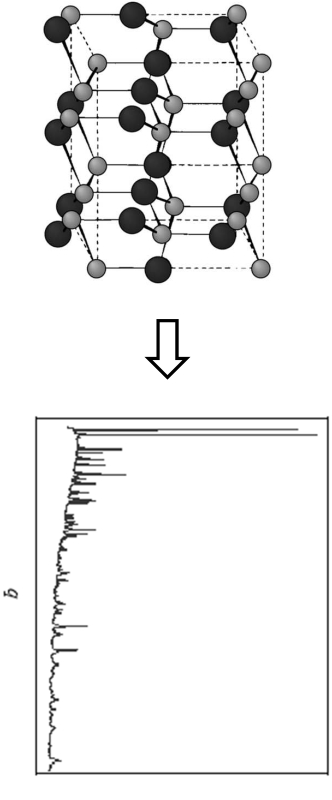
A function $\wp$ on ${\mathbb{R}}^{N}$ is said to be periodic if $L:=\{l\in{\mathbb{R}}^{N}:\wp(x+l)=\wp(x)\text{ for any }x\in{\mathbb{R}}^{N}\}$ is a lattice. We call $L$ the period lattice of $\wp$. For example, an electron (or nucleus) density in a crystal (cf. the left figure in Figure 4) is a periodic function of $N=3$.

The following $\wp$ provides its standard model.

where

According to diffraction theory, if a crystal has an electron density $\wp$, the diffraction image of its single-crystal sample equals $cf_{single}(x^{*};\wp)$ for some $c>0$, where $f_{single}(x^{*};\wp)$ is a sum of delta functions given by

A powder sample is an ensemble of a very large number of randomly oriented crystallites. As a result, its diffraction image is proportional to the integration of $f_{single}(x^{*};\wp)$ on a sphere of radius $\sqrt{q}$:

The $\hat{\wp}(l^{*})$ is called a structure factor in crystallography.

The right figure in Figure 4 presents an actual powder diffraction pattern. It is obtained by replacing every delta function in (7) with some kind of peak-shape model function $g$ that is close to a Gaussian distribution and satisfies $\int_{{\mathbb{R}}}g(q)dq=1$.

Ab-initio powder crystal structure determination retrieves the electron density $\wp$ from the powder diffraction pattern under the assumption that the following additional information is available.

• •

  chemical formula (i.e., the ratio $[d_{1}:\cdots:d_{m}]$),

• •

  density of a single crystal,

• •

  rapidly decreasing functions $p_{i}$ ($1\leq i\leq m$).

Powder auto-indexing is the initial stage of ab-initio powder crystal structure determination, and aims to find the period lattice $L$ of $\wp$. As the positions of the delta functions, elements of $\Lambda_{\wp}$ are extracted from a powder diffraction pattern $f_{powder}(q;\wp)$.

$L$ is normally determined from elements of $\Lambda_{\wp}$ in powder auto-indexing. After $L$ is obtained, using the coefficients $F_{\wp}(q)$, powder crystal structure determination is carried out.

In this section, we formulate the problem explicitly. In powder auto-indexing, extracted $\Lambda^{obs}$ is different from the set $\Lambda^{\wp}$ of true ${\left\lvert l^{*}\right\rvert}^{2}$ ($l^{*}\in L^{*}$) owing to observational problems. Consequently, the Gram matrix $S$ of the period lattice $L$ of $\wp$ must be retrieved from $\Lambda^{obs}$ under the following assumptions.

1. ($A$1)

   The observed range of a powder diffraction pattern is contained in a finite interval $[q_{min},q_{max}]\subset(0,\infty)$. Consequently, only information about $\Lambda_{\wp}\cap[q_{min},q_{max}]$ is available.

2. ($A$2)

   Every $q^{obs}\in\Lambda^{obs}$ has some observation error. It may be assumed that the threshold ${\rm Err}[q^{obs}]$ on the error ${\left\lvert q^{obs}-q^{cal}\right\rvert}$ is given. (A method to compute ${\rm Err}[q^{obs}]$ is introduced in [22].)

3. ($A$3)

   Owing to probabilistic mistakes and errors in acquisition of the peak-positions (i.e., peak-search), $\Lambda^{obs}$ differs from the true $\Lambda_{\wp}\cap[q_{min},q_{max}]$. There exist small $\epsilon_{1}>0$ and $\epsilon_{2}>0$ satisfying the following conditions:

   1. (i)

      For arbitrarily fixed $q\in\Lambda_{\wp}\cap[q_{min},q_{max}]$, the following occurs with probability $\epsilon_{1}$:

      $\displaystyle q\notin\bigcup_{q^{obs}\in\Lambda^{obs}}[q^{obs}-{\rm Err}[q^{obs}],q^{obs}+{\rm Err}[q^{obs}]].$

      (10)

   2. (ii)

      For arbitrarily fixed $q^{obs}\in\Lambda^{obs}$, the following occurs with probability $\epsilon_{2}$:

      $\displaystyle\Lambda_{\wp}\cap[q^{obs}-{\rm Err}[q^{obs}],q^{obs}+{\rm Err}[q^{obs}]]=\emptyset.$

      (11)

4. ($A$4)

   When the distribution $\wp$ is constrained by group symmetry, infinitely many $\hat{\wp}(l^{*})$ and $F_{\wp}(q)$ become zero owing to systematic absences deterministically (Section 4).

As assumed in (3), $\Lambda_{obs}$ extracted from a powder diffraction pattern has missing or false elements. These are caused by observational problems including background noise or false peaks due to sample impurity.

With regard to (4), sometimes $F_{\wp}(q)=0$ holds due to a special arrangement of atom positions $x_{ik}$, rather than systematic absences (cf. [12], [27]). However, the probability is zero if every $x_{ik}$ is distributed uniformly in ${\mathbb{R}}^{N}/L$. (The only known exceptions are systematic absences.)

For the special arrangement with zero probability, we replace $\Lambda_{\wp}$ by $\Lambda_{ext}(\wp)$ and consider ($\tilde{A}$3) instead of ($A$3):

1. ($\tilde{A}$3)

   Assume that

   1. (i)

      For any $q\in\Lambda_{ext}(\wp)\cap[q_{min},q_{max}]$, $q\notin\bigcup_{q^{obs}\in\Lambda^{obs}}[q^{obs}-{\rm Err}[q^{obs}],q^{obs}+{\rm Err}[q^{obs}]]$ occurs with probability $\epsilon_{1}$.

   2. (ii)

      For any $q^{obs}\in\Lambda^{obs}$, $\Lambda_{ext}(\wp)\cap[q^{obs}-{\rm Err}[q^{obs}],q^{obs}+{\rm Err}[q^{obs}]]=\emptyset$ occurs with probability $\epsilon_{2}$.

Under the conditions ($A$1)–($A$4), infinitely many solutions may exist in some cases (for example, consider the case of very small $[q_{min},q_{max}]$). Hence, additional assumptions are necessary in order to guarantee a finite number of solutions.

1. ($A$5)

   Owing to repulsive force between atoms, we may assume $\min\{|l|^{2}:0\neq l\in L\}\geq d^{2}$ for a positive constant $d\approx 2\AA$. Then, by the inequalities on successive minima of $L$ and its reciprocal lattice $L^{*}$ proved by Lagarias et al. [17], in $N=2,3$, the maximum diagonal entry $D_{N}$ of a Minkowski-reduced(defined in Appendix C) Gram matrix $S$ of $L^{*}$ satisfies

   $\displaystyle D_{N}\leq\frac{N+3}{4d^{2}}\max\{\gamma_{i}:1\leq i\leq N\},$

   (13)

   where $\gamma_{i}$ is the Hermite constant:

   $\displaystyle\gamma_{i}:=\sup\left\{\min\{\hskip 1.42262pt{}^{t}\hskip-1.42262ptvSv:0\neq v\in{\mathbb{Z}}^{N}\}:S\in{\mathcal{S}}^{i}_{\succ 0},\ {\rm det}S=1\right\}.$

   (14)

   In particular, $D_{2}\leq\frac{5}{3}d^{-2}$ and $D_{3}\leq 3\cdot 2^{-1/3}d^{-2}$ follow from $\gamma_{1}=1$, $\gamma_{2}^{2}=\frac{4}{3}$, $\gamma_{3}^{3}=2$. (In $N=2$, the estimation is improved up to $D_{2}\leq\frac{4}{3}d^{-2}$ easily.)

2. ($A$6)

   The length of the interval $\sqrt{q_{max}}-\sqrt{q_{min}}$ is sufficiently greater than $\sqrt{D_{N}}$ that there exists $l_{1}^{*}$, $l_{2}^{*}$, $l_{3}^{*}$ is a basis of $L^{*}$ such that $\Lambda^{obs}$ includes ${\left\lvert l_{1}^{*}\pm l_{2}^{*}\right\rvert}^{2}$, ${\left\lvert l_{1}^{*}\pm l_{3}^{*}\right\rvert}^{2}$, ${\left\lvert\pm l_{1}^{*}+l_{2}^{*}+l_{3}^{*}\right\rvert}^{2}$, and at least one of the following for both $i=2,3$:

   1. (i)

      ${\left\lvert l_{1}^{*}\right\rvert}^{2}$, ${\left\lvert l_{i}^{*}\right\rvert}^{2}$,

   2. (ii)

      ${\left\lvert l_{1}^{*}\right\rvert}^{2},{\left\lvert l_{1}^{*}-2l_{i}^{*}\right\rvert}^{2}$,

   3. (iii)

      ${\left\lvert l_{1}^{*}\right\rvert}^{2},{\left\lvert l_{1}^{*}+2l_{i}^{*}\right\rvert}^{2}$,

   4. (iv)

      ${\left\lvert l_{i}^{*}\right\rvert}^{2},{\left\lvert 2l_{1}^{*}-l_{i}^{*}\right\rvert}^{2}$.

   5. (v)

      ${\left\lvert l_{i}^{*}\right\rvert}^{2},{\left\lvert 2l_{1}^{*}+l_{i}^{*}\right\rvert}^{2}$.

In ($A$5), $2\AA$ is selected as the minimum distance between the two closest latttice points of $L$ satisfied by any existing crystals. ($A$6) looks rather artificial. This assumption is necessary for our algorithm in Table 5. By Theorems 2 and 3, ($A$6) holds except for events with zero probability if a sufficiently large $q_{max}$ is chosen, regardless of the type of systematic absences. Under assumptions ($A$5) and ($A$6), the number of solutions is always finite, because $\Lambda^{obs}\subset[q_{min},q_{max}]$ contains only finite elements and the Gram matrix of $L^{*}$ is computed from a combination of elements of $\Lambda^{obs}$ due to assumption ($A$6).

Here, it is still non-trivial how to select $q_{max}$. At least, it is clear $q_{max}\geq D_{3}$ is required; otherwise $\Lambda_{ext}(\wp)\cap[q_{min},q_{max}]$ contain only ${\left\lvert l^{*}\right\rvert}^{2}$ of $l^{*}\in L_{2}^{*}$ in some cases, where $L_{2}^{*}\subset L^{*}$ is a sublattice of rank less than 3. On the other hand, as seen in (3) in Section 8, too many $q$-values are frequently extracted from the interval $[q_{min},D_{3}]$ when we set $d=2\AA$ and $D_{3}:=3\cdot 2^{-1/3}d^{-2}$, nevertheless powder auto-indexing is very frequently successful even with a smaller interval. Since the time of our enumeration algorithm is roughly proportional to the fourth power of the number of elements of $\Lambda^{obs}$ (cf. Section 7.3), the time can be significantly decreased by minimizing the range $[q_{min},q_{max}]$. Considering the current accuracy of diffractometers and the power of personal computers, $q_{max}$ should be chosen empirically to some degree, in addition to the theoretical estimation above. See (3) in Section 8.1 for a more detailed approach to this issue.

We now give some definitions for crystallographic groups and systematic absences. In the following, we represent the elements $x\in{\mathbb{R}}^{N}/L$ as a row vector and $l^{*}\in L^{*}$ as a column vector. Furthermore, any group action on ${\mathbb{R}}^{N}/L$ (resp. $L^{*}$) is represented as a right action (resp. left action).

Any congruent transformation of the Euclidean space ${\mathbb{R}}^{N}$ is represented as a composition of the orthogonal group $O(N)$ and a translation; if $\sigma$ is a congruent transformation of ${\mathbb{R}}^{N}$, there exist $\tau\in O(N)$ and $\nu\in{\mathbb{R}}^{N}$ such that:

Such a $\sigma$ is denoted by $\{\tau|\nu\}$. The group consisting of all congruent transformations of ${\mathbb{R}}^{N}$ is the semidirect group $O(N)\ltimes{\mathbb{R}}^{N}$. By expanding the composition $(x^{\{\tau_{1}|\nu_{1}\}})^{\{\tau_{2}|\nu_{2}\}}$, it is seen that the group multiplication is given by:

A crystallographic group is also called a wallpaper group in $N=2$, and a space group in $N=3$.

For a crystallographic group $G$, two groups $R_{G}$ and $L$ are defined by:

where $1_{N}$ is the identity of $O(N)$. $L$ is a lattice and $R_{G}$ is a finite subgroup of $O(N)$ consisting of $\tau$ that maps any elements of $L$ to $L$. $R_{G}$ is called a point group of $G$. $G$ is a group extension of $L$ by $R_{G}$. From the definition of $L$, for any $\{\tau|\nu_{\tau}\}\in G$, the class $\nu_{\tau}+L\in{\mathbb{R}}^{N}/L$ is uniquely determined. Furthermore, the map $R_{G}\longrightarrow{\mathbb{R}}^{N}/L$ : $\tau\mapsto\nu_{\tau}+L$ is a $1$-cocycle, i.e., it satisfies

We now proceed to the definition of systematic absences. Let $G$ be a crystallographic group with the point group $R_{G}$ and the translation group $L$, and consider the following periodic function $\wp$:

Note that the density model function $\wp$ in (4), is represented as in (20) for some space group $G$.

Let $L^{2}({\mathbb{R}}^{N})$ be the $L^{2}$-space, i.e., the set of all measurable functions $f$ on ${\mathbb{R}}^{N}$ with a finite $L^{2}$-norm $||f||_{2}:=(\int_{{\mathbb{R}}^{N}}{\left\lvert f(x)\right\rvert}^{2}dx)^{1/2}<\infty$. In order to compute the same list as [14], let us assume that

(Isotropy condition) $p_{i}$ belongs to $L^{2}({\mathbb{R}}^{N})^{R_{G}}$, i.e., $p_{i}(x^{\tau})=p_{i}(x)$ holds for any $\tau\in R_{G}$.

Then, $\wp(x^{\sigma})=\wp(x)$ holds for any $\sigma\in G$, and $\wp$ has the Fourier coefficient

where $\hat{p}_{i}(l^{*}):=\int_{{\mathbb{R}}^{N}}p_{i}(x)e^{-2\pi\sqrt{-1}x\cdot l^{*}}dx$.

Hence, the probability of $\hat{\wp}(l^{*})=0$ depends on the size of $W_{G,l^{*}}\subset{\mathbb{R}}^{N}/L$.

In the following, we shall focus on $\Gamma_{ext}(G,H)$, since we have $\Gamma_{ext}(G)=\Gamma_{ext}(G,\{id\})$. From the definition, it is clear that $-l^{*}$ and $\tau l^{*}$ belong to $\Gamma_{ext}(G,H)$ for any $\tau\in R_{G}$ if and only if $l^{*}$ does.

For $\wp$ in (20) satisfying the isotropy condition, it is not difficult to confirm that the following equivalence condition holds when $H_{i}\subset G$ is the stabilizer subgroup of $x_{i}\in{\mathbb{R}}^{N}$:

As proved by Bieberbach [2], [3], a homomorphism $\varphi:G_{1}\longrightarrow G_{2}$ is an isomorphism between two crystallographic groups $G_{1}$ and $G_{2}$ if and only if there is an affine map $\alpha$ of ${\mathbb{R}}^{N}$ such that $\varphi(g)=\alpha g\alpha^{-1}$. For such $G_{1},G_{2}$, $\Gamma_{ext}(G_{1},H)=\Gamma_{ext}(G_{2},\varphi(H))$ clearly holds. In general, we also have $\Gamma_{ext}(G,H)=\Gamma_{ext}(G,\sigma H\sigma^{-1})$ for any $\sigma\in G$.

$\Gamma_{ext}(G,H)$ is computed using the following proposition.

References

• [1] M. Bhargava and J. Hanke. Universal quadratic forms and the 290 theorem. Invent. Math., 2005.
• [2] L. Bieberbach. Über die bewegungsgruppen der euklidischen räume. Mathematische Annalen, 70(3):297–336, 1911.
• [3] L. Bieberbach. Über die bewegungsgruppen der euklidischen räume (zweite abhandlung.) die gruppen mit einem endlichen fundamentalbereich. Mathematische Annalen, 72(3):400–412, 1912.
• [4] A. Boultif and D. Louër. Powder pattern indexing with the dichotomy method. J. Appl. Cryst., 37:724–731, 2004.
• [5] J. W. S. Cassels. Rational Quadratic Forms. Academic Press, London/New York, 1978.
• [6] J. H. Conway. The sensual (quadratic) form. Carus Mathematical Monographs 26, Mathematical Association of America, 1997.
• [7] J. H. Conway and N. J. A. Sloane. Low-dimensional lattices vi: Voronoi reduction of three-dimensional lattices. Proc. Royal Soc. London, Series A, 436:55–68, 1992.
• [8] J. H. Conway and N. J. A. Sloane. Sphere Packings, Lattices and Groups (3rd ed.), volume 290 of Grundlehren der mathematischen Wissenschaften. Springer, 1998.
• [9] P. M. de Wolff. On the determination of unit-cell dimensions from powder diffraction patterns. Acta Cryst., 10:590–595, 1957.
• [10] P. M. de Wolff. Detection of simultaneous zone relations among powder diffraction lines. Acta Cryst., 11:664–665, 1958.
• [11] P. M. de Wolff. A simplified criterion for the reliability of a powder pattern indexing. J. Appl. Cryst., 1:108–113, 1968.
• [12] P. Engel, T. Matsumoto, G. Steinmann, and H. Wondratschek. The non-characteristic orbits of the space groups. Z. Kristallogr., Supplement Issue No. 1, 1984.
• [13] P. M. Gruber and S. S. Ryshkov. Facet-to-facet implies face-to-face. European Journal of Combinatorics, 10:83–84, 1989.
• [14] T. Hahn. International tables for Crystallography, volume A. Dordrecht:Kluwer, 1983.
• [15] T. Ito. A general powder x-ray photography. Nature, 164:755–756, 1949.
• [16] M. Kac. Can one hear the shape of a drum? American Mathematical Monthly, 73(4):1–23, 1966.
• [17] J. C. Lagarias, H. W. Lenstra, JR., and C. P. Schnorr. Korkin-zolotarev bases and successive minima of a lattice and its reciprocal lattice. COMBINATORICA, 10(4):333–348, 1990.
• [18] A. Le Bail. Monte carlo indexing with McMaille. Powder Diffraction, 19:249–254, 2004.
• [19] Y. S. Moon. Universal quadratic forms and the 15-theorem and 290-theorem. Thesis (Stanford University), 2008.
• [20] M. A. Neumann. X-cell: a novel indexing algorithm for routine tasks and difficult cases. J. Appl. Cryst., 36(4):356–365, 2003.
• [21] P. Niggli. Kristallographische und strukturtheoretische Grundbegriffe. Handbuch der Experimentalphysik, volume 7. Leipzig: Akademische Verlagsgesellschaft, 1928.
• [22] R. Oishi-Tomiyasu. Rapid bravais-lattice determination algorithm for lattice parameters containing large observation errors. Acta Cryst. A., 68:525–535, 2012.
• [23] S. S. Ryshkov and E. P. Baranovskii. C-types of n-dimensional lattices and 5-dimensional primitive parallelohedra (with application to the theory of coverings). Proceedings of the Steklov Institute of Mathematics, 137, 1976.
• [24] A. Schiemann. Ein beispiel positiv definiter quadratischer formen der dimension 4 mit gleichen darstellungszahlen. Archiv der Mathematik, 54:372–375, 1990.
• [25] A. Schiemann. Ternary positive definite quadratic forms are determined by their theta series. Mathematische Annalen, 308:507–517, 1997.
• [26] E. Selling. Über die binären und ternären quadratischen formen. J. Reine Angew. Math., 77:143–229, 1874.
• [27] D. H. Templeton. Systematic absences corresponding to false symmetry. Acta Cryst., 9:199–200, 1956.
• [28] F. Vallentin. Sphere coverings, lattices, and tilings (in low dimensions). PhD thesis, Technical University Munich, Germany, 2003.
• [29] J. W. Visser. A fully automatic program for finding the unit cell from powder data. J. Appl. Crystallogr., 2:89–95, 1969.
• [30] G. F. Voronoi. Sur quelques proprietes des formes quadratiques positives parfaites. J. Reine Angew. Math., 133:97–178, 1907.
• [31] G. F. Voronoi. Nouvelles applications des parametres continus a la theorie des formes quadratiques. J. Reine Angew. Math., 134:198–287, 1908.
• [32] G. L. Watson. Determination of binary quadratic form by its values at integer points. MATHEMATIKA, 26:72–75, 1979.
• [33] G. L. Watson. Determination of binary quadratic form by its values at integer points: Acknowledgement. MATHEMATIKA, 27:188, 1980.
• [34] P.-E. Werner, L. Eriksson, and M. Westdahl. Treor, a semi-exhaustive trial-and-error powder indexing program for all symmetries. J. Appl. Cryst., 18:367–370, 1985.