Three-Band Model for Quantum Hall and Spin Hall Effects
Abstract
Topological properties of a certain class of spinless three-band Hamiltonians are shown to be summed up by the Skyrmion number in momentum space, analogous to the case of two-band Hamiltonian. Topological tight-binding Hamiltonian on a Kagome lattice is analyzed with this view. When such a Hamiltonian is “folded”, the two bands with opposite Chern numbers merge into a degenerate band exhibiting non-Abelian gauge connection. Conserved pseudo-spin current operator can be constructed in this case and used to compute the pseudo-spin Hall conductance. Our model Hamiltonians belong to the symmetry class D and AI according to the ten-fold classification scheme.
I Introduction
Topological properties embedded within a band structure have emerged as one of the central themes of condensed matter physics nowadays. The topological nature is often expressed as the gauge field derived from the underlying wave functions and manifests itself in such observable phenomena as anomalous and spin Hall effects in metals [1, 2]. Quantized versions of the phenomena exist in insulators, when a certain topological number can be associated with the completely filled bands. Classification of the permissible topological numbers in a given band Hamiltonian was recently carried out [3]. Numerous efforts are being made at the moment to suggest specific models belonging to a particular entry in the classification table with relevance to realizable experimental systems. A most striking instance of this kind of effort is Haldane’s proposal of microscopic two-band Hamiltonian with spontaneous quantized Hall conductance [4], its generalization to time-reversal-invariant quantum spin Hall phase [5, 6], and its subsequent realization in HgTe/CdTe heterostructure [6, 7].
Basically, spontaneous quantum Hall models and a subset of quantum spin Hall models defined as two time-reversal copies of the quantum Hall model can be phrased as a property of the generic two-band Hamiltonian , where is a two-component spinor and the matrix is (=Pauli matrix). As long as the -vector remains nonzero over the entire Brillouin zone (BZ) such that a unique unit-vector exists, the two eigenstates of will be classified according to their spin helicity . From the Abelian gauge connection the associated flux density can be written in two equivalent forms,
| (1) |
Quantized number for the band, obtained as the integral of Eq. (1), can therefore be interpreted as either the first Chern number or the Skyrmion number of the given band [8, 9, 10] depending on the use of the second or the third term of Eq. (1) for the integrand.
There are quite a few other models embodying nontrivial topological numbers that involve the use of 44 -matrices, many of which are summarized in Ref. 3. Although the general classification scheme makes no reference to the dimensionality of the matrix itself, in practice almost all explicit examples of band Hamiltonians with nontrivial topology take the form of an even-dimensional matrix in momentum space. In sharp contrast, general discussion of the topological character for odd-dimensional 33 matrices, or three-band Hamiltonians, appear to be lacking. The work of Ohgushi, Murakami, and Nagaosa (OMN) [11] provided, to the authors’ knowledge, the first microscopic example of a three-band model Hamiltonian with non-trivial topological Chern number. The three-sublattice structure of the Kagome lattice is a natural platform for the three-dimensional Hamiltonian matrix to arise.
In this paper, we divide the general three band Hamiltonian into the spin-1 part and nematic part then try to solve each part separately. The spin-1 model and nematic model involve quantum Hall effect and spin Hall effect respectively. In contrast to two band model, for the spin-1 model, the first Chern number is one half of skyrmion number. We realize that the existence of half-skyrmion (meron) configuration for a unit Chern number band. When we consider the Kagome lattice models for the nematic model, which the spin matrices represent the pseudo-spin from the three-sublattice structure, our spin Hall effect describes the pseudo-spin Hall effect.
The remaining part of this paper is organized as follows. In Sec. II, in terms of spin-1 matrices, we consider a particular three band model involving the quantum Hall effect. All of the other three band model is topologically equivalent to spin-1 model unless the band gap is closed. As a realistic example, we introduce the OMN model on Kagome lattice which has unit Chern number including the meron structure in momentum space. In Sec. III, by introducing the nematic operator, we construct the different type of three band model with time-reversal symmetry which involves the (pseudo-)spin Hall effect. For an specific model based on Kagome lattice, we perform the linear response calculation of the (pseudo-)spin Hall conductivity. Then we give an physical interpretation for our (pseudo-)spin Hall effect. In Sec. IV we conclude with brief summary and discussions.
II Spin-1 model
In general, arbitrary three-band Hamiltonian can be written as a linear combination of eight Gell-Mann matrices (), , characterized by eight-component real field . Due to its complicate structure, the exact analytical solution of general three band model is difficult to obtain. By the way, as is well-known, Gell-Mann matrices are the generators of the SU(3) Lie algebra which possess as subgroups several sets of three matrices forming SU(2), or SO(3) sub-algebra. In particular the subset that generates the SO(3) rotation are the matrices of spin-1 operators. We will show that the subset of 33 Hamiltonians spanned by the SO(3) generators can be readily analyzed in analogous fashion as their 22 counterparts. We specialize to three-band Hamiltonians of the type
| (2) |
where one possible choice of the spin-1 matrix S would be , or :
| (3) |
All other choices of SO(3) subgroup elements ought to be related to this by a suitable unitary transformation. As in the two-band Hamiltonian, we assume remains nonzero throughout the BZ. The eigenstates of energies and can be worked out readily in terms of the unit vector [12, 13],
The state of energy is the complex conjugate of : .
With the aid of explicit wave functions one can evaluate the gauge flux associated with each band. The central band, having real-valued wave functions, has the zero flux, while the upper band has the flux density[12]
| (11) |
The lower band has the opposite sign of the flux density. Comparing Eq. (11) to Eq. (1) one notes a difference of factor 2, originating from spin-1 being twice the size of spin-1/2 [12]. A full Skyrmion for in the BZ will thus imply an even Chern number for the spin-1 bands.
We ask now if certain topological three-band models considered in earlier literature can be framed in the form of the “parent Hamiltonian” plus some perturbation. As long as the parent model is connected smoothly to the full one without the gap closing the topological property will be completely captured by the relation, Eq. (11). The Kagome lattice model of OMN [11] is
| (12) |
where , , while and for the three unit vectors of the Kagome lattice shown in Fig. 1(d). The flux penetrating the triangle unit of the Kagome lattice is compensated for by flux through the hexagon in the OMN model. We have verified that does not close the energy gap of the parent Hamiltonian , provided the flux satisfies the condition . The Skyrmion number associated with the -vector of the parent OMN Hamiltonian is readily obtained, , giving rise to the Chern number for the upper band according to Eq. (11). The Chern number obtained for the same band in Ref. 11 is , equal to our result provided . This is precisely the same condition required for the topological equivalence of the original OMN model to its parent form. Written in real space lattice the parent Hamiltonian gives the hopping amplitude proportional to for every nearest neighbor bond traversed in the counter-clockwise direction.

An astute reader may wonder how come the Skyrmion number in the parent OMN Hamiltonian is only half of an integer. In fact any Hamiltonian matrix that shares the periodicity of the first BZ, i.e. for reciprocal lattice vector , will only allow the integer Skyrmion numbers due to the homotopy and, by virtue of Eq. (11), only even Chern integers. On the other hand, explicit calculation of the Berry phase flux yields the Chern numbers of [11]. So why the apparent contradiction? A closer examination shows that for the OMN model is not periodic under but rather under as shown graphically in Fig. 1(a). The same relation between Chern number and winding number for three orbital model with the spin-1 representation is studied in Ref. 12. As a result, is equivalent to only up to some constant, -independent unitary rotation: . By evading the periodic condition the Hamiltonian becomes exempt from the usual homotopy consideration as well, making the half Skyrmion configuration possible. In fact with a different choice of the basis the OMN matrix can be written in such a way that holds. In that case, however, the model can no longer be reduced to the form and the Skyrmion number interpretation of the Chern number fails to apply [14].
Topological nature of the spin-1 Hamiltonian can be phrased in the general classification scheme of Ref. 3. Under complex conjugation one has and . The Hamiltonian possesses time-reversal symmetry (TRS) and/or particle-hole symmetry (PHS) if some unitary transformation could relate to (TRS) or (PHS), respectively. When the -vector is even, , we further have , hence the TRS/PHS amounts to the existence of unitary transformation , respectively. It follows that SLS is trivially satisfied with , while TRS cannot be achieved with any . This places our Hamiltonian (2) in the D class [3], where the allowed topological numbers are the integers in two spatial dimensions, equal to the Chern numbers we just calculated. If instead we had the Hamiltonian would have TRS but not PHS, placing it in class AI, without any topological numbers. Indeed one can easily show that for the -vector of odd symmetry the Skyrmion number vanishes identically.
III Nematic model
So far the discussion of the topological character of three-band Hamiltonian is restricted to the “spin” type given by Eq. (2). The nomenclature is obviously derived from being a representation of spin. On the other hand, the following observation prompts us to study another class of three-band Hamiltonians that we denote the “nematic” type. Note that the anti-commutators of the three spin operators generate the following five:
These are precisely the remaining five of the Gell-Mann matrices, or in the language of spin liquids, the nematic operators. An arbitrary 3-band Hamiltonian is therefore a sum of the spin part and the nematic part, , where the five components of refer to the above five operators and is a five-component function of . The Hamiltonian consisting solely of the nematic operators are real, , and TRS/PHS conditions become . In this case even (odd) generates the AI (D) class Hamiltonian [3].
A particularly simple kind of nematic Hamiltonian arises by folding the previous spin Hamiltonian
| (14) |
The folding ensures the degeneracy of Kramers’ pairs with the identical energy wherein non-Abelian gauge connection arises [15, 16, 17, 18]. The same wave functions worked out before the folding remain as eigenstates of the new Hamiltonian. A similar three-band Hamiltonian, with , was proposed for the -orbital bands of Si [18]. An example of the folded four-band model employing the spin operator is the Luttinger Hamiltonian, extensively studied by Murakami, Nagaosa, and Zhang as a model for dissipationless spin Hall current in GaAs [16, 17]. Even for spinless models such as ours, an analogue of spin Hall current can be defined and its response function computed. The special case of was analyzed in Ref. [18]. Here we maintain the framework as general as possible by keeping an arbitrary non-zero vector over the BZ.
Each band has the associated helicity number, () and the band-dependent flux density,
| (15) |
The sum of Chern numbers for the doubly degenerate band is obviously zero. Regarding as the pseudo-spin matrix, the projected pseudo-spin density may be defined as [16, 17, 18]
| (16) |
with and denoting the projection onto the eigenstates with and , respectively, and is the three-component spinor consisting of A, B, C sublattice site operators. Together with the projected spin current operator
| (17) |
they obey the continuity equation . The d.c. pseudo-spin Hall conductivity follows as (=volume) [17, 18]
| (18) |
where is the Fermi function of each band . Here stands for the direction of the applied electric field, the spatial direction of spin current, and is the spin orientation. This formula is general and applicable to any three-band Hamiltonians of the folded form, Eq. (14). Numerical evaluation of the pseudo-spin Hall conductance for the parent OMN model is shown in Fig. 1(e). Due to symmetry other spin orientations give the same Hall conductance: .
Intuitive understanding of the pseudo-spin Hall conductance follows from the fact that spin operator we use also serves as the sublattice current operator. For instance, expressed in the sublattice basis becomes , equal to orbital current operator for that bond. As a whole we may identify in obvious notation. The eigenstate has the average , and with our new interpretation it implies that the current loop around a ABC triangle shown in Fig. 2(a) is and minus this value for . These opposite current loops are the analogues of opposite spin orientations in the genuine spin Hall effect. Now these current loops of opposite signs move in the opposite directions due to the opposite signs of the gauge flux they experience, conserving the time-reversal invariance, and result in the pseudo-spin Hall phenomena (Fig. 2(b)).

Imposing boundaries in the -direction at and at as shown in Fig. 1(d) introduces some edge modes. The topologically protected edge modes [19] of the parent OMN model connecting the topological bands (top and bottom) with the non-topological band (center) as shown in Fig. 1(c) obey the dispersion [20] when the hopping magnitude is chosen to one. The folded Hamiltonian also support edge modes, albeit unprotected in the topological sense, with the dispersion as shown in Fig. 1(d). The explicit derivation of the edge dispersion is presented in the Appendix. For the OMN model the sign of the velocity determines the spatial location of the edge as either or . In the folded case both edge modes obey the same energy dispersion. The absence of protected edge mode connecting the degenerate bands to the flat band is due to the net topological number for the former bands being zero [19, 21].
IV Conclusion and Discussion
In this paper we have taken up the study of the topological aspects of three-band Hamiltonian, applicable to spinless fermions and bosons with three-fold orbital or sublattice degree of freedom. As with the topological two-band models, the Hall conductances of the three-band Hamiltonian is shown to be governed by the same (Chern number) (Skyrmion number) correspondence with a critical difference of factor two allowing for the existence of meron structure in momentum space for three-band Hamiltonians. For the OMN model we succeeded in obtaining the topological number of the model by using the parent model of Eq. (2). However, we didn’t mention about how to obtain the parent model from the general three band model. In this point, we need further studies. A second class of three-band Hamiltonians obtained by the folding procedure is studied. The double degeneracy ensured by folding naturally leads to non-Abelian gauge structure and spin Hall phenomena. Both of three-band models we study, before and after the folding, are subject to the symmetry classification scheme of Ref. 3.
Acknowledgements.
J. H. H. is supported by NRF grant (No. 2010-0008529, 2011-0015631). We acknowledge informative discussions with H. Katsura, Dung-Hai Lee, E. G. Moon, and N. Nagaosa. *Appendix A Edge modes in the folded model
In the OMN model, the chiral edge state is obtained in Ref. 20. Here we calculate the edge mode solutions of the folded OMN model,
| (1) |
where
| (2) |
The real space expression of the Hamiltonian is obtained by writing down its Fourier transformation,
| (3) |
In order to obtain the edge states, we should choose a particular boundary condition. The boundary condition is depicted in Fig. 1 (d). Since the system is no longer periodic along the direction, is not good quantum number. Let us consider momentum representation in direction
| (4) |
Here, we used . Inserting the one particle state
| (5) |
into the Schrodinger equation , we have the one-dimensional chain equations of [19]
| (6) | ||||
| (7) | ||||
| (8) |
with the boundary conditions
| (9) |
For exponentially localized solutions on the boundaries we take the ansatz [22]
| (10) |
with the condition . Thus we can write as
| (11) |
where is real function of momentum . Putting this all together we obtain the edge solutions as
| (12) |
with
| (13) |
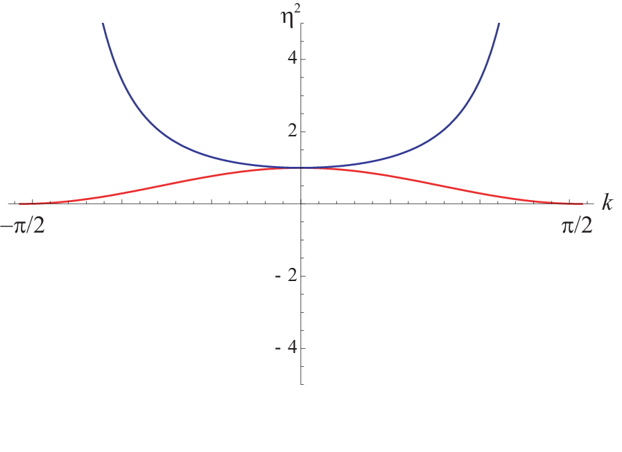
The degenerate edge spectrum are depicted in Fig. 1 (c). For (), the edge state is localized at upper(lower) edge.
References
- [1] Naoto Nagaosa, Jairo Sinova, Shigeki Onoda, A. H. MacDonald, and N. P. Ong, Rev. Mod. Phys. 82, 1539 (2010).
- [2] Di Xiao, Ming-Che Chang, and Qian Niu, Rev. Mod. Phys. 82, 1959 (2010).
- [3] Andreas P. Schnyder, Shinsei Ryu, Akira Furusaki, and Andreas W. W. Ludwig, Phys. Rev. B 78, 195125 (2008); New J. Phys. 12, 065010 (2010).
- [4] F. D. M. Haldane, Phys. Rev. Lett. 61, 2015 (1988).
- [5] C. L. Kane and E. J. Mele, Phys. Rev. Lett. 95, 146802 (2005); ibid. 95, 226801 (2005).
- [6] B. Andrei Bernevig, Taylor L. Hughes, and Shou-Cheng Zhang, Science 314, 1757 (2006).
- [7] Markus König, Steffen Wiedmann, Christoph Brune, Andreas Roth, Hartmut Buhmann, Laurens W. Molenkamp, Xiao-Liang Qi, and Shou-Cheng Zhang, Science 318, 766 (2007).
- [8] G.E. Volovik, Sov. Phys. JETP 67, 1804-1811 (1988).
- [9] Wu-Yi Hsiang and Dung-Hai Lee, Phys. Rev. A 64, 052101 (2001).
- [10] Xiao-Liang Qi, Yong-Shi Wu, and Shou-Cheng Zhang, Phys. Rev. B 74, 085308 (2006).
- [11] Kenya Ohgushi, Shuichi Murakami, and Naoto Nagaosa, Phys. Rev. B 62, 6065 (2000).
- [12] Yan He, Joel Moore and C. M. Varma, Phys. Rev. B 85, 155106 (2012).
- [13] The wave function for contains a singularity at . Another wave function can be easily constructed for where the singularity appears elsewhere on the unit sphere[12].
- [14] We are grateful to Dung-Hai Lee for bringing this point out.
- [15] Frank Wilczek and A. Zee, Phys. Rev. Lett. 52, 2111 (1984).
- [16] Shuichi Murakami, Naoto Nagaosa, and Shou-Cheng Zhang, Science 301, 1348 (2003).
- [17] Shuichi Murakami, Naoto Nagaosa, and Shou-Cheng Zhang, Phys. Rev. B 69, 235206 (2004).
- [18] B. Andrei Bernevig, Taylor L. Hughes, and Shou-Cheng Zhang, Phys. Rev. Lett. 95, 066601 (2005).
- [19] Yasuhiro Hatsugai, Phys. Rev. Lett. 71, 3697 (1993).
- [20] Alexandru Petrescu, Andrew A. Houck, and Karyn Le Hur, arXiv:1206.1539 (2012).
- [21] Masaru Onoda and Naoto Nagaosa, Phys. Rev. Lett. 95, 106601 (2005).
- [22] M. Creutz and I. Horvath, Phys. Rev. D 50, 2297 (1994).