Cosmological moduli problem in large volume scenario and thermal inflation

One of the most attractive features of low energy supersymmetry (SUSY) is the unification of gauge couplings at the scale $M_{\rm GUT}\sim 10^{16}\mathinner{\mathrm{GeV}}$. The GUT scale is two orders of magnitude smaller than the Planck scale, and this hierarchy may be understood within a higher dimensional setup of string theory, in which gravity lives in a relatively large bulk spacetime, while GUT degrees of freedom are confined on branes [1]. Such scenario then requires a moduli stabilization scheme which would stabilize the overall volume modulus at a large value in string unit.

An attractive scheme realizing large compactification volume is the large volume scenario (LVS) of [2], proposed in the context of type IIB string theory. This scheme involves two Kähler moduli, $T_{b}$ and $T_{s}$, where $\tau_{b}={\rm Re}(T_{b})$ corresponds to a 4-cycle volume modulus determining the bulk Calabi-Yau volume as ${\cal V}\simeq\tau_{b}^{3/2}$, and $\tau_{s}={\rm Re}(T_{s})$ describes a small 4-cycle volume supporting a nonperturbative superpotential of the form $W_{\rm np}\sim e^{-aT_{s}}$. The interplay between $W_{\rm np}$ and a perturbative correction to the Kähler potential suppressed by $1/\tau_{b}^{3/2}$ determines the VEV of $\tau_{b}$ as

which can be exponentially large for a moderately large value of $a\tau_{s}$. In LVS, the hierarchy between the Planck scale and the GUT scale is given by [3]

so $\tau_{b}=\mathcal{O}(10^{4})$ results in the correct hierarchy between the GUT scale and the Planck scale.

The large VEV of the volume modulus implies that its scalar potential is relatively flat (at least near the minimum), so the volume modulus is relatively light. Specficially, the mass of the large volume modulus in LVS is given by

which would be in the range of cosmological care unless the gravitino mass $m_{3/2}$ is heavy enough to ensure $m_{\tau_{b}}\gtrsim 100$ TeV. Cosmologically, huge amount of moduli can be produced in the form of a coherent oscillation after primordial inflation, so in general light moduli cause disasters due to their too late decays. Depending on their life-times, they could destruct light elements formed at BBN, produce too much $X$ ($\gamma$)-rays, distort CMBR or provide too much relic density [4, 5]. One way out of this cosmological moduli problem is raising-up of the moduli masses, so that moduli can decay before BBN. For this, the volume modulus should be heavier than about $100\mathinner{\mathrm{TeV}}$ as usual moduli should. For $\tau_{b}={\cal O}(10^{4})$, such heavy volume modulus would require $m_{3/2}\gtrsim 10^{9}$ GeV, and therefore a careful sequestering of gravity mediated SUSY breaking if one wishes to realize low energy SUSY in the visible sector with soft SUSY breaking masses $m_{\rm soft}\sim 1$ TeV [6].

On the other hand, considering various possible higher order corrections, either in $\alpha^{\prime}$ or in the string coupling, it is likely to be difficult to realize a sequestering which would allow $m_{\rm soft}/m_{3/2}\sim 10^{-6}$ [7, 8, 9]. In case that an enough sequestering is not achieved, the large volume modulus becomes relatively light, and then the most compelling solution to the cosmological moduli problem is a late thermal inflation [10]. As primordial inflation does, thermal inflation can wipe out pre-existing particles, for example, moduli. However it works in a limited sense, since energy density of thermal inflation itself becomes a source of moduli reproduction. Depending on the mass of moduli, such a reproduction could be fatal, and the large volume scenario could be in cosmological trouble.

In this paper, we study the cosmological moduli problem of LVS for the gravitino mass range

which corresponds to the volume modulus mass range

for $\tau_{b}=\mathcal{O}(10^{4})$. We show that, if inflaton decays before the large volume modulus starts to oscillate, single thermal inflation can solve the problem only for a limited range of $m_{\tau_{b}}$. Particularly, the volume modulus mass range $m_{\tau_{b}}=\mathcal{O}(10^{-2}-1)\mathinner{\mathrm{GeV}}$, which would be the case if gravity mediated SUSY breaking is not sequestered well, is difficult to be cosmologically viable with single thermal inflation only. On the other hand, if inflaton decays just before thermal inflation begins, the abundance of moduli can be minimized, so the whole range of $m_{\tau_{b}}$ can be viable with a single-step thermal inflation. However, such a very late decay of inflaton is not typical, so we consider a double-step thermal inflation as an alternative solution, and show that the problem can be solved in a natural manner. It turns out that correct amounts of baryon asymmetry and dark matter can be obtained also via a late-time Affleck-Dine leptogenesis [11, 12, 13, 14, 15] and the decay of the visible sector NLSP to flatino LSP.

This paper is organized as follows. In section 2, we briefly review LVS and the properties of moduli. In section 3, cosmological moduli problem in LVS is discussed. In section 4, it is argued that single thermal inflation is not enough to solve the cosmological moduli problem for certain range of the volume modulus mass. We then clarify the conditions for a double-step thermal inflation to be realized, while solving the cosmological moduli problem for the entire modulus mass range in consideration. In section 5, considering a specific model for the mediation of SUSY breaking, which involves $D$-term mediation associated with anomalous $U(1)$ gauge symmetry and also the conventional gauge mediation, we demonstrate that a double-step thermal inflation can be realized in a natural manner and solve the cosmological problem of the light volume modulus. We also show that the model can produce correct amounts of baryon asymmetry and dark matter too. Section 6 is the conclusion.

In this section, we review briefly the large volume compactification and properties of moduli involved.

The basic properties of LVS models can be viewed from a simple model in 4D supergravity (SUGRA) framework. The model is characterized by the following Kähler potential and superpotential [2]

where $\tau_{I}={\rm Re}(T_{I})$ ($I=b,s$) are the Kähler moduli determining the size of the Calabi-Yau (CY) volume as ${\cal V}=\tau_{b}^{3/2}-\tau_{s}^{3/2}$, and $K$ is expanded in powers of $1/\tau_{b}$. The $\xi$-term is the stringy $\alpha^{\prime}$ correction and given by $\xi_{\alpha^{\prime}}=\zeta(3)\chi(M)/\left[2g_{s}^{3/2}\left(2\pi\right)^{3}\right]$ with $\chi(M)$ and $g_{s}$ being the Euler number of the CY manifold and string coupling, respectively. $W_{0}$ is the tree-level flux superpotential from the stabilization of the dilaton and complex structure moduli. $A_{s}$, the flux dependent constant, can be taken to be real value by shift transformation of $T_{s}$: $T_{s}\rightarrow T_{s}+i\alpha$. Then, one finds that the SUGRA scalar potential at large volume limit is given by

This potential has a SUSY-breaking AdS minimum at

Since it is known that possible uplift process to get dS vacuum does not change the vacuum properties related to our argument, we do not care about that in this paper. The masses of the moduli are given by

where $M_{\mathrm{P}}=2.4\times 10^{18}\mathinner{\mathrm{GeV}}$ is the reduced Planck scale,

are the canonically normalized scalar fields of $T_{s}$ and $T_{b}$, respectively, $\psi_{s}$ and $\psi_{b}$ are their fermionic superpartners, $m_{3/2}=e^{K/2}|W|\simeq|W_{0}|/\tau_{b}^{3/2}$ is the gravitino mass. A generic feature of moduli masses in LVS is that the mass of the large volume modulus is suppressed by a power of $1/\tau_{b}$ compared to $m_{3/2}$, reflecting the fact that the no-scale structure of the scalar potential is approximately preserved in the large volume limit. The enhancement or suppression factor, the power of $\ln(M_{\mathrm{P}}/m_{3/2})$, in the mass spectrum (9) is a consequence of the non-perturbative corrections which have a crucial role in moduli stabilization.

In order to know the real values of the moduli masses, we have to specify the vacuum value of $\tau_{b}$ and the gravitino mass. In the context of local GUT models, for universal tree-level gauge kinetic functions $f_{a}$, the running gauge coupling constants are unified at scale $M_{\rm GUT}\sim M_{\mathrm{P}}/\tau_{b}^{1/2}$ [17, 3]. Therefore, the hierarchy between the GUT and Planck scales can be naturally obtained for $\tau_{b}\sim 10^{3}-10^{5}$ as

The gravitino mass is an order parameter of SUSY breaking, and its value is related with soft SUSY breaking masses for the visible sector, $m_{\rm soft}={\cal O}(1\,{\rm TeV})$, by SUSY breaking mediation mechanism. In the mixed $D$-term-gauge mediation which will be discussed in our paper, $m_{\rm soft}$ is just of the order of $m_{3/2}$. In other mediation mechanism, such as small volume modulus mediation $(m_{\rm soft}\sim m_{3/2}/8\pi^{2}$) [2] whose mass hierarchy is similar to that of [16] as a general result for the SUSY breaking moduli stabilized by non-perturbative superpotential, and $U(1)_{A}$ threshold corrections ($m_{\rm soft}\sim m_{3/2}/\sqrt{8\pi^{2}}$) [9] in which the soft mass squared is generated at one-loop order due to the SUSY breaking mass spectrum of the $U(1)_{A}$ vector superfield, there can be hierarchy between $m_{3/2}$ and soft terms. On the other hand, as discussed in [6], if the visible sector is far from the small 4-cycle governing by $\tau_{s}$, and the possible loop corrections are quite suppressed, then tree-level gravity mediation induces the soft parameters much suppressed compared to the gravitino mass as $m_{\rm soft}\sim m_{3/2}/\tau_{b}^{3/2}$. ^** * In this type of model, the typical sfermion mass $m_{\varphi_{i}}$ is of order of $m_{\phi_{b}}\sim m_{3/2}/\tau_{b}^{3/4}$, while the gaugino mass $M_{a}$ is of ${\cal O}(m_{3/2}/\tau_{b}^{3/2})$. In order for $m_{\varphi_{i}}$ to be the same order of $M_{a}$, we need further sequestering as $e^{-K/3}Z_{i}\sim 1+{\cal O}(1/\tau_{b}^{3})$, where $Z_{i}$ is the matter Kähler metric, or $m_{\varphi_{i}}^{2}$ is given by $(\partial V/\partial\phi_{b})/M_{\mathrm{P}}+{\cal O}(m_{3/2}^{2}/\tau_{b}^{3})$ so that $\langle m_{\varphi_{i}}^{2}\rangle={\cal O}(m_{3/2}^{2}/\tau_{b}^{3})$. Thus, here we allow the gravitino mass in the range of

that gives

The life-time of a modulus is determined by interactions with its superpartners and ordinary matter fields localized in small cycles. In the latter case, most important parts are the Kähler metric and the gauge kinetic function for the visible sector

where $\Phi_{i}$s are the matter chiral superfields, $T_{v}$ is the Kähler modulus determining the visible sector 4-cycle volume, and ($\cdots$) denotes higher order terms. $T_{v}$ can not be identified as $T_{b}$, if not, it provides too small gauge coupling constants. This is the phenomenological reason why the matter fields should be localized in a small cycle. In this case, the functional form of the Käher metric is given by $Z_{i}\simeq{\cal Y}_{j}(\tau_{s},\tau_{v})/\tau_{b}$. Then, it is straightforward to calculate the coefficients of the following interaction terms between the large volume modulus and the visible sector fields:

The visible-sector gauge field strength is denoted by $F^{a\mu\nu}$, $\lambda^{a}$ is the superpartner of the gauge field, the gaugino. $\varphi_{i}$ and $\psi_{i}$ are the scalar and fermion component of $\Phi_{i}$, respectively. $m_{\varphi_{i}}^{2}$ and $b_{\varphi_{ij}}$ are quadratic mass parameters for sfermions coming from SUSY breaking and supersymmetric contributions, respectively. $M_{a}$ is the gaugino mass, $m_{\psi_{i}}$ is the fermion mass for $\psi_{i}+\psi_{i}^{c}$. The model dependent coefficients are generically

Let us briefly discuss the origin of each terms. At a tree-level, the interactions between $\phi_{b}$ and gauge fields are rather suppressed, because $f_{a}$ in Eq. (15) does not have $T_{b}$ dependence. However, due to the Konishi and the super-Weyl anomaly, three point interactions are generated at the one-loop level [17]. Thus $\beta_{a}$ is generically ${\cal O}(1/8\pi^{2})$. $\tilde{c}_{i}$, $\tilde{c}_{ij}$ and $c_{a}$ are mostly originated from the soft SUSY breaking mass terms that depend on $\phi_{b}$ as $m_{\rm soft}\sim M_{\mathrm{P}}/\tau_{b}^{n_{b}}\sim M_{\mathrm{P}}\exp(-n_{b}\phi_{b}/M_{\mathrm{P}})$, where $n_{b}$ is the constant determined by SUSY breaking and its mediation mechanism, so generically they are of order unity. In some cases, there are terms like $(\partial V/\partial\phi_{b})/M_{\mathrm{P}}$ in $m_{\varphi_{i}}^{2}$ and $b_{\varphi_{ij}}$, which are vanishing by equations of motion so that the contribution to the soft masses are zero. However, the interation between the modulus and the scalar fields are extracted as $(\partial^{2}V/\partial^{2}\phi_{b})\,\delta\phi_{b}\,|\varphi_{i}|^{2}/M_{\mathrm{P}}\sim m_{\phi_{b}}^{2}\delta\phi_{b}|\varphi_{i}|^{2}/M_{\mathrm{P}}$. As a result, $\tilde{c}_{i}$, and $\tilde{c}_{ij}$ can be enhanced by a factor of $m_{\phi_{b}}^{2}/m_{\rm soft}^{2}$ for $m_{\phi_{b}}\gg m_{\rm soft}$.^†† † It can be shown that we can take a field basis such that derivative interactions between $\phi_{b}$ and ($\varphi_{i},\,\psi_{i}$) are absent. Then, all interactions are obtained from the potential terms. This basis is good in the sense that we do not need to care about cancelations between the interactions obtained from the kinetic part and potential part. $c_{i}$ depends on the origin of the fermion mass term. Through the Higgs bilinear $\mu$-parameter and soft masses, the Higgs can interact with $\phi_{b}$. Due to the non-zero vacuum value of the Higgs fields, there is a mixing between the Higgs and $\phi_{b}$ in the mass eigenbasis. Then, the SM fermions can interact with $\phi_{b}$ through the modulus-Higgs mixing. Higgsinos can directly interact with $\phi_{b}$ via $\mu H_{u}H_{d}$ term in the superpotential or from the Kähler potential by Giudice-Masiero mechanism [18]. In addition, the large volume modulus can decay to axion $a_{b}$, the complex counter part of the modulus, with a sizable branching fraction via kinetic term.

All those interactions are suppressed by Planck scale with additional suppression factors depending on channels. The decay rates of $\phi_{b}$ to daughter particles are given by

provided the decay channels are kinematically allowed. Note that decays to matter fields is at most comparable to the axion channel though it depends on models. Note also that the branching fraction of the large volume modulus to photons is suppressed by $\mathcal{O}(10^{-4})$ relative to that of axion channel.

On the other hand, the strength of interactions between the small volume modulus and the matter fields is much more enhanced compared to that for the large volume modulus. Because, as in Eq. (10), $\delta\tau_{s}\sim\delta\phi_{s}/M_{\rm st.}$ with $M_{\rm st}\simeq M_{\mathrm{P}}/\tau_{b}^{3/4}$ being the string scale in large volume scenario, the suppression scale of the interaction between $\phi_{s}$ and matters is not Planck scale, but string scale [19]. As a result, in case that $T_{v}$ and $T_{s}$ have a sizable mixing at the tree-level, the small volume modulus mostly decays to the gauge boson pair as

where $\gamma_{s\to A_{\mu}^{a}A_{\mu}^{a}}$ is a numerical coefficient of $\mathcal{O}(10)$ taking the number of allowed channels into account.

The abundance of a modulus is highly constrained, depending on its life-time. The small volume modulus decays dominantly to SM particles well before BBN epoch, hence it is harmless as long as right amounts of baryon number asymmetry and dark matter can be obtained. In case of the large volume modulus, the life-time can be written as

where ${\rm Br}_{\phi_{b}\to a_{b}a_{b}}$ is the branching fraction to large volume axions and always sizable for all mass range of $\phi_{b}$. For $m_{\phi_{b}}\lesssim 100\mathinner{\mathrm{TeV}}$, the large volume modulus decays around or after BBN epoch. In this case, as listed below, there are various constraints depending on the life-time, $\tau_{\phi_{b}}$.

• •

  $\tau_{\phi_{b}}\lesssim 0.1\sec$: The relic abundance is restricted by the effective number of the extra relativistic degrees of freedom, $\Delta N_{\rm eff}$, to which the primordial abundance of ⁴He, D is highly sensitive. Contribution from moduli decay is

  $$\Delta N_{\rm eff}=\frac{\rho_{a_{b}}}{\rho_{\nu}}=\frac{1-{\rm Br}(\phi_{b}\to{\rm SM})}{{\rm Br}(\phi_{b}\to{\rm SM})\times g_{\nu}/g_{*}(T_{\rm d,\phi_{b}})}$$

  (21)

  where $g_{\nu}=7/4$ and $g_{*}(T_{\rm d,\phi_{b}})$ are the relativistic degrees of freedom of a left-handed neutrino and standard model particles (including neutrinos), respectively. The observed value, $\Delta N_{\rm eff}<1$ ($1\sigma$) from BBN [20] and $\Delta N_{\rm eff}=0.85^{+0.39}_{-0.56}$ ($1\sigma$) from BBN+CMB+LSS [21], poses a constraint, ${\rm Br}_{\rm SM}\gtrsim 0.9$. Such a sizable branching fraction can be achieved if $\tilde{c}_{i}\,(\tilde{c}_{ij})\sim m_{\phi_{b}}^{2}/m_{\rm soft}^{2}$ [22]. Otherwise, for $\tilde{c}_{i}(\tilde{c}_{ij})\sim 1$, ${\rm Br}_{\rm SM}\ll 1$, and moduli should be a sub-dominant energy component of the universe when they decay. Actually, the constraint from the extra radiation contribution to the SM radiation is applicable for the moduli decaying in a present Hubble time though $g_{\nu}$ has to be replaced to $g_{\nu}\times(4/11)^{4/3}$ for $\tau_{\phi_{b}}\gtrsim 1\sec$. However, the constraint is weaker than others described below.

• •

  $0.1\sec\lesssim\tau_{\phi_{b}}\lesssim 10^{12}\sec$: The direct interaction between decay products of $\phi_{b}$ and the background light elements causes significant changes in the abundances of light elements from the predictions by standard BBN [23]. If $\tau_{\phi_{b}}\gtrsim 10^{6}\sec$, it also affects the CMB spectrum as a deviation from the Planck distribution [24]. The corresponding constraint is, however, rather milder than that from the abundance of ³He/D.

• •

  $10^{12}\sec\lesssim\tau_{\phi_{b}}\lesssim 10^{24}\sec$: In this case, moduli decay after the recombination era. The most stringent constraint is coming from the diffused X($\gamma$)-ray [5, 25]. For the life-time longer than the age of the universe ($\tau_{\phi_{b}}\gtrsim 10^{17}\sec$), X($\gamma$)-ray produced in the galactic center should be also considered.

• •

  $\tau_{\phi_{b}}\gtrsim 10^{24}\sec$: In this case, the only constraint is from the present dark matter relic density, $\Omega_{\rm DM}h^{2}\simeq 0.11$ [26].

All these constraints are shown in Fig. 1 where we see that, for $10\mathinner{\mathrm{MeV}}\lesssim m_{\phi_{b}}\lesssim 100\mathinner{\mathrm{TeV}}$, the abundance of the light modulus is constrained to be less than

that corresponds to

where $n_{\phi_{b}}$ and $s$ are the number density of the light modulus and entropy density, respectively.

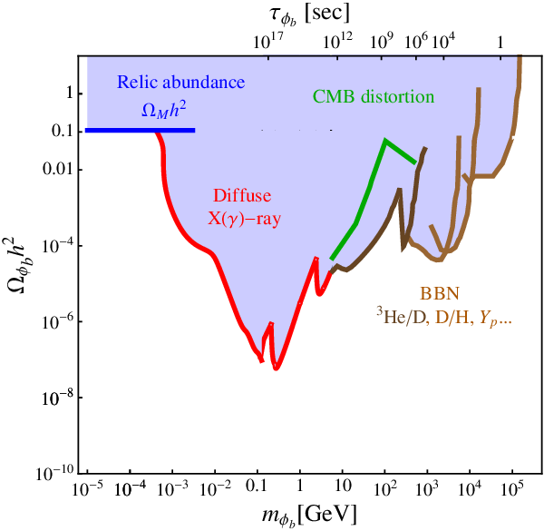
The cosmological moduli problem is that the typically expected moduli abundance is much larger than the upper bounds shown in Fig. 1. In the very early universe, when the expansion rate becomes comparable to the mass of a modulus, the modulus is expected to be produced enormously in the form of coherent oscillation caused by vacuum misalignment. In case of the small volume modulus, the initial oscillation amplitude is expected to be string scale, and the modulus never dominates the universe until it decays well before BBN. Hence it is harmless. On the other hand, the large volume modulus has Planckian initial oscillation amplitude ^‡‡ ‡ The initial misalignment of $\phi_{b}$ might be typically super-Planckian. For such a large field value, the potential is of an exponential form. Then, in the universe dominated by radiation it will be quickly attracted to near its vacuum position [27]. Once $\Delta\phi_{b}\lesssim M_{\mathrm{P}}$ with respect to the vacuum position, the potential can be approximated as a quadratic form, and the modulus oscillates with an amplitude of order Planck scale and behaves like a matter. Therefore, we can simply assume that the initial misalignment of the light modulus is of order Planck scale when it starts to oscillate in a radiation dominated universe. , and dominates the universe right after it starts to oscillate or at least when it decays.

We assume that the expansion rate during the primordial inflation is much larger than the mass of the small modulus. The light modulus starts to oscillate when $H\sim m_{\phi_{b}}$. Denoted as $Y\equiv n_{\phi_{b}}/s$, the late-time abundance of the light modulus is given by

where $T_{\rm R}$ is the reheating temperature of inflaton and defined as

with $\Gamma_{I}$ being its decay rate, and we assumed that the energy density of the modulus is equal to that of inflaton for $\Gamma_{I}\lesssim m_{\phi_{b}}$. If $\Gamma_{I}\gtrsim m_{\phi_{b}}$, the late-time entropy release in the decay of heavy moduli, $\phi_{s}$, can dilute the abundance of the light modulus by a factor

at most. Hence the late-time abundance of the light modulus after the decay of the small volume modulus is

where we used $\tau_{b}\simeq 10^{4}$ and $\ln(M_{\mathrm{P}}/m_{3/2})\simeq 4\pi^{2}$. If $\Gamma_{I}<m_{\phi_{b}}$, we find

since the reheating temperature of inflation should be larger than about $1\mathinner{\mathrm{MeV}}$ for successful BBN. As shown in Eqs. (27) and (28), irrespective of the reheating temperature of inflation, the abundance of the large volume modulus is too much to match the observational constraints, Eq. (23). Hence, the light modulus causes a disaster in a consistent cosmology unless its abundance is somehow diluted enough.

The most compelling solution to the cosmological moduli problem is thermal inflation [10]. In this section, we show that single thermal inflation is only a partial solution to the moduli problem in LVS for the mass scale of moduli(Eq. (14)), though it depends on the reheating temperature of the primordial inflation. We then consider a double thermal inflation as a complete solution to the problem, and clarify how it works.

References

- (1) E. Witten, Nucl. Phys. B 471, 135 (1996) [hep-th/9602070].
- (2) V. Balasubramanian, P. Berglund, J. P. Conlon and F. Quevedo, JHEP 0503 (2005) 007 [arXiv:hep-th/0502058]; J. P. Conlon, F. Quevedo and K. Suruliz, JHEP 0508 (2005) 007 [arXiv:hep-th/0505076].
- (3) J. P. Conlon, JHEP 0904, 059 (2009). [arXiv:0901.4350 [hep-th]]; J. P. Conlon, E. Palti, Phys. Rev. D80, 106004 (2009). [arXiv:0907.1362 [hep-th]].
- (4) G. D. Coughlan, W. Fischler, E. W. Kolb, S. Raby and G. G. Ross, Phys. Lett. B 131, 59 (1983); T. Banks, D. B. Kaplan and A. E. Nelson, Phys. Rev. D 49, 779 (1994) [hep-ph/9308292]; B. de Carlos, J. A. Casas, F. Quevedo and E. Roulet, Phys. Lett. B 318, 447 (1993) [hep-ph/9308325];
- (5) J. Hashiba, M. Kawasaki and T. Yanagida, Phys. Rev. Lett. 79, 4525 (1997) [arXiv:hep-ph/9708226]; T. Asaka, J. Hashiba, M. Kawasaki and T. Yanagida, Phys. Rev. D 58, 083509 (1998) [arXiv:hep-ph/9711501]; K. Choi, E. J. Chun and H. B. Kim, Phys. Rev. D 58, 046003 (1998) [hep-ph/9801280].
- (6) R. Blumenhagen, J. P. Conlon, S. Krippendorf, S. Moster, F. Quevedo, JHEP 0909, 007 (2009). [arXiv:0906.3297 [hep-th]]
- (7) J. P. Conlon, F. G. Pedro, JHEP 1006, 082 (2010). [arXiv:1003.0388 [hep-th]].
- (8) K. Choi, H. P. Nilles, C. S. Shin, M. Trapletti, JHEP 1102, 047 (2011). [arXiv:1011.0999 [hep-th]].
- (9) C. S. Shin, JHEP 1201, 084 (2012) [arXiv:1108.5740 [hep-ph]].
- (10) D. H. Lyth and E. D. Stewart, Phys. Rev. Lett. 75, 201 (1995) [hep-ph/9502417]; D. H. Lyth, E. D. Stewart, Phys. Rev. D53, 1784-1798 (1996). [hep-ph/9510204].
- (11) E. D. Stewart, M. Kawasaki and T. Yanagida, Phys. Rev. D 54, 6032 (1996) [arXiv:hep-ph/9603324].
- (12) D. h. Jeong, K. Kadota, W. I. Park and E. D. Stewart, JHEP 0411, 046 (2004) [arXiv:hep-ph/0406136]. M. Kawasaki, K. Nakayama, Phys. Rev. D74, 123508 (2006). [hep-ph/0608335].
- (13) G. N. Felder, H. Kim, W. I. Park and E. D. Stewart, JCAP 0706, 005 (2007) [arXiv:hep-ph/0703275];
- (14) S. Kim, W. I. Park and E. D. Stewart, JHEP 0901, 015 (2009) [arXiv:0807.3607 [hep-ph]];
- (15) K. Choi, K. S. Jeong, W. I. Park and C. S. Shin, JCAP 0911, 018 (2009) [arXiv:0908.2154 [hep-ph]]; W. -I. Park, JHEP 1007, 085 (2010). [arXiv:1004.2326 [hep-ph]]; K. Choi, E. J. Chun, H. D. Kim, W. I. Park and C. S. Shin, Phys. Rev. D 83, 123503 (2011) [arXiv:1102.2900 [hep-ph]].
- (16) K. Choi, A. Falkowski, H. P. Nilles, M. Olechowski and S. Pokorski, JHEP 0411, 076 (2004) [arXiv:hep-th/0411066]; K. Choi, A. Falkowski, H. P. Nilles and M. Olechowski, Nucl. Phys. B 718, 113 (2005) [arXiv:hep-th/0503216].
- (17) V. Kaplunovsky and J. Louis, Nucl. Phys. B 422, 57 (1994) [hep-th/9402005].
- (18) G. F. Giudice and A. Masiero, Phys. Lett. B 206, 480 (1988).
- (19) J. P. Conlon and F. Quevedo, JCAP 0708, 019 (2007) [arXiv:0705.3460 [hep-ph]].
- (20) G. Mangano and P. D. Serpico, Phys. Lett. B 701, 296 (2011) [arXiv:1103.1261 [astro-ph.CO]].
- (21) J. Hamann, S. Hannestad, G. G. Raffelt and Y. Y. Y. Wong, JCAP 1109, 034 (2011) [arXiv:1108.4136 [astro-ph.CO]].
- (22) M. Cicoli, J. P. Conlon and F. Quevedo, arXiv:1208.3562 [hep-ph]; T. Higaki and F. Takahashi, arXiv:1208.3563 [hep-ph].
- (23) K. Jedamzik, Phys. Rev. D 70 (2004) 063524 [astro-ph/0402344]; M. Kawasaki, K. Kohri and T. Moroi, Phys. Lett. B 625 (2005) 7 [astro-ph/0402490]; M. Kawasaki, K. Kohri and T. Moroi, Phys. Rev. D 71 (2005) 083502 [astro-ph/0408426].
- (24) W. Hu and J. Silk, Phys. Rev. Lett. 70, 2661 (1993). J. C. Mather, E. S. Cheng, D. A. Cottingham, R. E. Eplee, D. J. Fixsen, T. Hewagama, R. B. Isaacman and K. A. Jesnsen et al., Astrophys. J. 420, 439 (1994); D. J. Fixsen, E. S. Cheng, J. M. Gales, J. C. Mather, R. A. Shafer and E. L. Wright, Astrophys. J. 473, 576 (1996) [astro-ph/9605054].
- (25) E. Churazov, R. Sunyaev, M. Revnivtsev, S. Sazonov, S. Molkov, S. Grebenev, C. Winkler and A. Parmar et al., [astro-ph/0608250]; A. W. Strong, I. V. Moskalenko and O. Reimer, Astrophys. J. 613, 956 (2004) [astro-ph/0405441]; A. W. Strong, I. V. Moskalenko and O. Reimer, Astrophys. J. 613, 962 (2004) [astro-ph/0406254]. A. A. Abdo et al. [Fermi-LAT Collaboration], Phys. Rev. Lett. 104, 101101 (2010) [arXiv:1002.3603 [astro-ph.HE]].
- (26) J. Beringer et al. (Particle Data Group), Phys. Rev. D 86, 010001 (2012).
- (27) J. P. Conlon, R. Kallosh, A. D. Linde and F. Quevedo, JCAP 0809, 011 (2008) [arXiv:0806.0809 [hep-th]].
- (28) L. Anguelova, V. Calo and M. Cicoli, JCAP 0910, 025 (2009) [arXiv:0904.0051 [hep-th]].
- (29) D. E. Morrissey and J. D. Wells, Phys. Rev. D 74, 015008 (2006) [hep-ph/0512019].
- (30) J. E. Kim, Phys. Rev. Lett. 43 (1979) 103; M. A. Shifman, A. I. Vainshtein and V. I. Zakharov, Nucl. Phys. B 166 (1980) 493.
- (31) T. Moroi and K. Nakayama, Phys. Lett. B 703, 160 (2011) [arXiv:1105.6216 [hep-ph]].
- (32) R. Blumenhagen, S. Moster and E. Plauschinn, JHEP 0801, 058 (2008) [arXiv:0711.3389 [hep-th]].
- (33) M. Kawasaki, T. Takahashi and S. Yokoyama, JCAP 0912, 012 (2009) [arXiv:0910.3053 [hep-th]].