Gauge cooling in complex Langevin for QCD with heavy quarks
Abstract
We employ a new method, “gauge cooling”, to stabilize complex Langevin simulations of QCD with heavy quarks. The results are checked against results obtained with reweigthing; we find agreement within the estimated errors. The method allows us to go to previously unaccessible high densities.
pacs
11.15.Ha, 11.15BtIntroduction. – An important problem of particle physics is to derive the phase diagram of hot and dense QCD from first principles. The difficulty lies in the fact that the action becomes complex at finite density. Various methods have been employed to get around this problem: Taylor expansions at and analytic continuation from imaginary , reweighting etc., but these have a limited range of applicability [1]. A general method that recently has received a lot of attention is the Complex Langevin Equation (CLE) [2, 3, 4, 5, 6, 7, 8] . It has had some successes as well as some failures; the failures seem to be related to the problem that the system wants to spend “too much time too far out” in the complexified configuration space; this problem and possible ways to deal with it were discussed in [8, 9].
In QCD at finite density the enlarged gauge freedom in the complexified field space can actually open a new way to limit the dangerous large excursions by employing non-unitary gauge transformations. This freedom was used in a somehwat different way for a toy model [9]; the procedure used there, however, does not generalize to a lattice model in an obvious way.
Here we introduce the method of gauge cooling (g.c.), designed to keep the link variables as close as possible to the unitaries, thereby preventing the dangerous large excursions. We test the idea first for a simple Polyakov loop model, where we have exact results to compare our data with; then we apply it to a heavy quark approximation of QCD with chemical potential (HQCD) (cf. [7]).
Complex Langevin for gauge models – The complex Langevin method [10, 11] for a complex action is based on setting up a stochastic process on the complexification of the configuration space. The longtime average of holomorphic observables is then supposed to give the correct average corresponding to the complex weight . In lattice models of QCD the configuration space is (see [12] for the Real Langevin approach); after complexification this becomes [13]. The complex Langevin equation (CLE) is
| (1) |
are the Gell-Mann matrices; are independent Wiener increments, normalized as
| (2) |
is a differential operator (derivation) acting on functions of as
| (3) |
where means the variable has been replaced by with all other variables unchanged. The first term on the rhs of Eq.(1) (the drift term) is gauge covariant and transverse to the gauge orbits since is gauge invariant, but the noise term contains components along the gauge orbits. Since the gauge group is noncompact, the process (1) may go far from the unitary submanifold.
An Euler discretization of Eq.(1) (see also [6]) gives
| (4) |
where is the drift force and are independent Gaussian noises satisfying
| (5) |
Gauge cooling. – It is a well known problem of the CLE method that the system may drift too far out into the imaginary directions, causing numerical problems. To quantify the distance from unitarity we use the ‘unitarity norm’
| (6) |
which vanishes if and only if all the ’s are unitary.
Gauge invariance is the freedom to transform variables
| (7) |
for all links , where initially are unitary, but after complexification . We use this freedom to minimize the unitarity norm, without changing the observables. Concretely, we intersperse standard ‘dynamical’ Langevin sweeps with several ‘g.c. sweeps’. These are deterministic moves essentially in the direction opposite to the gradient of .
A maximally nonunitary gauge transformation at site in direction is given by
| (8) |
() for all , with all other link variables remaining unchanged. The ‘gauge gradient’ of in the direction at the lattice site is then
| (9) |
The g.c. updates of the configuration are given by
| (10) |
where ; determines the strength of the g.c. force, whereas is a discretization parameter as in Eq.(4). Note that even if is not small, Eq.(10) is still a gauge transformation; it just might not be optimal for reducing .
Polyakov loop model. – The Polyakov loop model is given by a 1D lattice consisting of links with periodic boundary conditions. Analytically it reduces to a one-link integral, but it is a useful laboratory to check the effect of g.c.. The action is given by
| (11) |
where we allow to be complex. Here we choose , ; will in general be complex. The observables of interest are , . The effect of the g.c. on is shown in Fig.1, where we vary of Eq.(10). In Fig. 2 we show the effect of varying on the distribution of the values of . We see that with too small the distribution has a ‘skirt’ of slow decay. From [8] we know that slow decay typically leads to incorrect results; a small skirt, however, does not lead to appreciable deviations from the exact values. The main point is that enough cooling leads to correct results, see Fig.1.
We also measured and with similar results, for up to ; it turns out that increasing requires an increase in cooling.


Heavy quark QCD (HQCD). – The model was first explored using the CLE without g.c. in [7] on small lattices and for moderate . It is defined by dropping all spatial hopping terms of the quarks; this amounts to simplifying the Wilson fermion determinant of lattice QCD with nonzero chemical potential to
| (12) |
where , , Det refers to the color degrees of freedom and
| (13) |
HQCD is described by the action
| (14) |
where is the Wilson plaquette action and antiperiodic b.c. in time are chosen for the fermions. We have
| (15) |
and similarly for the second factor in Eq.(12), where
| (16) |
A related model has been studied numerically by a reweighting (RW) technique to deal with the complex density in [14] (and more recently in [15]), where for larger and larger lattices the sign problem causes bad signal to noise ratios. See [14] for the general setting.
We simulate the model by the CLE on various lattices, with , various values of and , using Eq.(4) with . In some cases we use adaptive control for the dynamical stepsize and the number of cooling steps. The system is thermalized after a cold start up to Langevin time before taking averages.
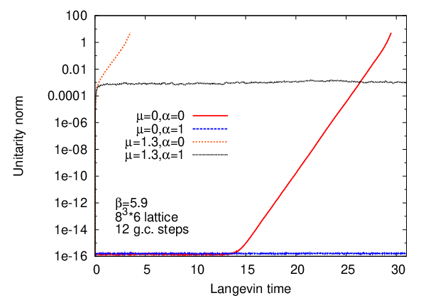
In Fig.3 we show the Langevin evolution of the unitarity norm: it is seen how g.c. stabilizes the process. We see that g.c. is needed even for where the process is real, but has an instability pushing it away from the unitary submanifold in the absence of cooling.
In Fig.4 we show the baryon density as a function of the chemical potential on an lattice. We find saturation for , suggesting that our results are correct also for fairly large . The figure also shows the average phase of , defined by
| (17) |
(see [7]). With growing density the average phase drops to almost zero and rises again in the saturation region.

Fig.5 shows and vs. . Both reach a maximum where the density takes off (), then drop again to nearly zero (see also [17, 18, 16]); the curve for is shifted slightly to the left with respect to . The analytic curves for in the figure exhibit a similar behavior; they are calculated essentially as in [14].
This behavior is due to the fact that for small as well as large the determinants in Eqs. (12) are dominated by the constant terms, leading to small expectation values of and . In physics terms, to get a nonzero answer one has to form a localized colorless bound state between the dynamical quarks and the external charge provided by or . For small , when typically there is only 1 quark present, it can form a ‘meson’ with but not with ; for larger , when typically 2 quarks are present, , but not can form a ‘baryon’ with them. The situation is slightly complicated by the fact that up to 6 quarks can exist at every site, so can also form a colorless state with 4 and with 5 quarks. With no quarks or in the completely filled state it is not possible to form such bound states. The simple picture given here ignores fluctuations, including a small probability, damped by , of finding antiquarks, so at and are small but nonzero, whereas at very large they will go to zero. Thus both quantities will have a peak, but will peak later than .

Comparison of CLE with RW. – To check the CLE results we also simulated HQCD with a RW technique, in the region where this is feasible (cf. [14]). We compare the results for the Polyakov loops and for plaquette expectations in Fig.6. The results agree within the errors (large errors only occur for RW). Note that around the RW method breaks down, whereas CLE with g.c. works fine for arbitrarily large .


In Fig.7 we show the expectation values of Polyakov loops at vs. , both obtained from RW and CLE. The figure shows that CLE works for large and also allows us to cross over into the confining region. Deeper in the confining region, however, we see small differences between the RW and CLE data, apparently related to an emergence of a ‘skirt’ of the distribution.
Concluding remarks. – The instabilities that arise without or with too weak g.c. are apparently caused by (1) the existence of repulsive fixed points, pushing the configurations exponentially fast away from the unitary submanifold and (2) roundoff and other numerical errors. Each gauge orbit contains configurations arbitrarily far from the unitaries, and there roundoff errors pile up to affect also the observables, violating gauge invariance.
The modified process remedies these problems; it thereby also avoids the slow decay of the equilibrium distribution. The CLE method with g.c. is tested successfully for the Polyakov loop model. It allows, apparently for the first time, to simulate a real QCD like gauge model at finite density all the way into the saturation region. The method does not suffer from any sign or overlap problem. There is no fundamental obstacle to extend the method to full QCD.
Acknowledgments. – We are grateful to Gert Aarts for discussions and collaboration in the early stage of the work; we also thank Frank James and Joyce Myers for useful discussions. I.-O. S. and E. S. were partly supported by Deutsche Forschungsgemeinschaft; I.-O. S. also thanks the Werner-Heisenberg-Institut for hospitality. A large part of the numerical calculations for this project was done on the bwGRiD (http://www.bw-grid.de), member of the German D-Grid initiative, funded by BMBF and MWFK Baden-Württemberg.
References
- [1] P. de Forcrand, PoS LAT 2009, 010 (2009) [arXiv:1005.0539].
- [2] J. Berges and I. -O. Stamatescu, Phys. Rev. Lett. 95 (2005) 202003 [hep-lat/0508030].
- [3] J. Berges, S. .Borsanyi, D. Sexty and I. -O. Stamatescu, Phys. Rev. D 75 (2007) 045007 [hep-lat/0609058].
- [4] C. Pehlevan and G. Guralnik, Nucl. Phys. B 811 (2009) 519 [arXiv:0710.3756]; G. Guralnik and C. Pehlevan, Nucl. Phys. B 822 (2009) 349 [arXiv:0902.1503].
- [5] G. Aarts and F. A. James, JHEP 1008 (2010) 020 [arXiv:1005.3468].
- [6] G. Aarts and F. A. James, JHEP 1201 (2012) 118 [arXiv:1112.4655].
- [7] G. Aarts and I. -O. Stamatescu, JHEP 0809 (2008) 018 [arXiv:0807.1597].
- [8] G. Aarts, E. Seiler and I. -O. Stamatescu, Phys. Rev. D 81 (2010) 054508 [arXiv:0912.3360]; G. Aarts, F. A. James, E. Seiler and I. -O. Stamatescu, Eur. Phys. J. C 71 (2011) 1756 [arXiv:1101.3270].
- [9] J. Berges and D. Sexty, Nucl. Phys. B 799 (2008) 306 [arXiv:0708.0779].
- [10] G. Parisi, Phys. Lett. 131 B (1983) 393.
- [11] J. Klauder, Acta Phys. Austr. Suppl. XXXV (1983) 251.
- [12] G. G. Batrouni, G. R. Katz, A. S. Kronfeld, G. P. Lepage, B. Svetitsky and K. G. Wilson, Phys. Rev. D 32 (1985) 2736.
- [13] H. Gausterer, Nucl. Phys. A642 (1998) 239c.
- [14] R. De Pietri, A. Feo, E. Seiler and I. -O. Stamatescu, Phys. Rev. D 76 (2007) 114501 [arXiv:0705.3420].
- [15] M. Fromm, J. Langelage, S. Lottini and O. Philipsen, JHEP 1201 (2012) 042 [arXiv:1111.4953].
- [16] M. Fromm, J. Langelage, S. Lottini, M. Neuman and O. Philipsen, [arXiv:1207.3005].
- [17] S. Hands, T. J. Hollowood and J. C. Myers, JHEP 1012 (2010) 057 [arXiv:1010.0790].
- [18] E. -M. Ilgenfritz and A. Maas, [arXiv:1210.5963].