Anisotropic Migdal-Eliashberg theory using Wannier functions
Abstract
We combine the fully anisotropic Migdal-Eliashberg theory with electron-phonon interpolation based on maximally-localized Wannier functions, in order to perform reliable and highly accurate calculations of the anisotropic temperature-dependent superconducting gap and critical temperature of conventional superconductors. Compared with the widely used McMillan approximation, our methodology yields a more comprehensive and detailed description of superconducting properties, and is especially relevant for the study of layered or low-dimensional systems as well as systems with complex Fermi surfaces. In order to validate our method we perform calculations on two prototypical superconductors, Pb and MgB2, and obtain good agreement with previous studies.
I INTRODUCTION
The prediction of superconducting properties such as the critical temperature or the superconducting energy gap remains one of the outstanding challenges in modern electronic structure theory. [1, 2, 3, 4, 5, 6, 7] Owing to the complex nature of the superconducting state, a quantitative understanding of the pairing mechanism in conventional superconductors requires a very detailed knowledge of the electronic structure, the phonon dispersions, and the interaction between electrons and phonons. In conventional superconductors below the critical temperature electron pairing results from a subtle interplay between the repulsive Coulomb interaction and the attractive electron-phonon interaction. Starting from the seminal work of Bardeen, Cooper, and Schrieffer (BCS) [8] several approaches to the calculation of the superconducting properties have been proposed, ranging from semi-empirical methods such as the McMillan formula, [9] to first-principles Green’s function methods such as the Migdal-Eliashberg (ME) formalism, [10, 11] and more recently also methods based on the density-functional theory concept, such as the density functional theory for superconductors (SCDFT). [6, 7]
The vast majority of current investigations rely on the semi-empirical McMillan’s approach. [9] In this approach the entire physics of the electron-phonon interaction is condensed into a single parameter called the electron-phonon coupling strength . The McMillan’s method works reasonably well for conventional bulk metals and for anisotropic superconductors where the Fermi surface anisotropy is smeared out by impurities. [2, 3] However, for layered systems, systems of reduced dimensionality, and those with complex multi-sheet Fermi surfaces, a careful description of the pairing interactions is crucial and a proper treatment of the anisotropic electron-phonon interaction is required. The necessity of an anisotropic theory has clearly been demonstrated in two important cases such as magnesium diboride, MgB2, and the graphite intercalation compound CaC6, using either the ME formalism or the SCDFT. [15, 17, 18, 12, 14, 13, 16]
Unfortunately, the lack of adequate computational tools prevents the research community from systematically exploring the importance of anisotropy in existing and well characterized superconductors, and for validating computational predictions based on the semi-empirical McMillan equation. [19, 20, 21, 22] This latter aspect is particularly relevant in view of the increasingly important role that high-throughput materials design approaches are acquiring in the community. [23, 24]
The momentum-resolved superconducting gap and the quasiparticle density of states near the Fermi surface can now be measured with unprecedented accuracy using high-resolution angle-resolved photoemission spectroscopy [25] and scanning tunneling spectroscopy [26] experiments. In this context, the anisotropic Migdal-Eliashberg formalism promises to be particularly useful for performing direct comparisons between theory and experiment, and for helping establish unambiguously the symmetry of the order parameter.
One critical point which arises when attempting to solve the Eliashberg equations of the ME theory or the Bogoliubov-de Gennes equations of the SCDFT is that both sets of equations suffer from a strong sensitivity to the sampling of the electron-phonon scattering processes in the vicinity of the Fermi surface. [27] The practical consequence of this sensitivity is that, in order to achieve numerical convergence, the electron-phonon matrix elements must be evaluated for extremely dense electron and phonon meshes in the Brillouin zone. This long-standing difficulty was overcome in Ref. 27 by developing an efficient first-principles interpolation technique based on maximally-localized Wannier functions (MLWF). [28] In this method one takes advantage of the spatial localization of both electron and phonon Wannier functions in order to evaluate only a small number of electron-phonon matrix elements in the Wannier representation. These matrix elements are subsequently interpolated to arbitrary electron and phonon wavevectors in the Bloch representation using a generalized Fourier transform. [27] This method carries general validity and has been demonstrated in several other areas, from Fermi surface calculations, [29] to the anomalous Hall effect,[30] and more recently for GW calculations. [31] A detailed introduction on Wannier-based interpolation methods can be found in Ref. 28. The scheme of Ref. 27 is adopted in the present work since it provides a robust and efficient framework for developing an algorithm to solve the anisotropic Eliashberg equations. Our current implementation enables the calculation of the momentum- and band-resolved superconducting gap using a very fine Brillouin zone sampling. Without our Wannier-based electron-phonon interpolation this operation would not be possible owing to the prohibitive computational cost.
This manuscript is organized as follows. In Sec. II we review the Migdal-Eliashberg theory of superconductivity. A description of the computational techniques underpinning the electron-phonon interpolation implemented in the EPW code [32] is given in Sec. III. In Sec. IV we report the numerical solutions of the Eliashberg equations for two prototypical superconductors, Pb and MgB2. Finally we present our conclusions and outlook in Sec. V.
II MIGDAL-ELIASHBERG FORMALISM
II.1 General theory
A quantitative theory of the superconducting energy gap can conveniently be formulated within the framework of the Nambu-Gor’kov formalism. [33, 34] In this formalism one introduces a two-component field operator:
| (1) |
The component () of the operator destroys (creates) an electron in a Bloch state of combined band and momentum index () and spin up (down). A generalized 22 matrix Green’s functions is then introduced in order to describe electron quasiparticles and Cooper’s pairs on an equal footing: [2, 4]
| (2) |
where is Wick’s time-ordering operator for the imaginary time and is obtained from Eq. (1) using the Heisenberg picture. The braces indicate a grand-canonical thermodynamic average. By replacing Eq. (1) inside Eq. (2) we find:
| (3) |
Here the diagonal elements correspond to the standard Green’s functions for electron quasiparticles and describe the dynamics of single-particle electronic excitations in the material. On the other hand, the off-diagonal elements represent Gor’kov’s anomalous Green’s functions and . These functions describe the dynamics of Cooper’s pairs and are related to the superconducting energy gap. [2, 4, 5] The off-diagonal elements of the generalized Green’s function in Eq. (3) become nonzero only below the critical temperature , marking the transition to the superconducting state.
The generalized Green’s function is periodic in imaginary time, therefore it can be expanded using a Fourier series as follows:
| (4) |
where ( integer) stands for the fermion Matsubara frequencies, and is the absolute temperature. We use atomic units throughout the manuscript, therefore we set . Following Eq. (4) the matrix elements of the generalized Green’s function read:
| (5) |
The study of the superconducting state involves the determination of the matrix Green’s function in Eq. (5). This can be achieved using Dyson’s equation:
| (6) |
where is the electron Green’s function for the normal state and is the self-energy associated with the pairing interaction. The normal-state Green’s function is calculated by using the Kohn-Sham states from density-functional theory to represent single-particle excitations. If we denote by the Kohn-Sham eigenvalues measured with respect to the chemical potential, and we introduce the Pauli matrices:
| (7) |
then the normal-state matrix Green’s function acquires the familiar form:
| (8) |
Within the Migdal-Eliashberg approximation the electron self-energy leading to the superconducting pairing consists of two terms, an electron-phonon contribution and a Coulomb contribution :[2]
| (9) |
with
| (10) | |||||
and
| (11) |
In Eq. (10) is the dressed propagator for phonons with momentum and branch index , and is the screened electron-phonon matrix element for the scattering between the electronic states and through a phonon with wavevector , frequency and branch index . In Eq. (11) the ’s represent the matrix elements of the static screened Coulomb interaction between the electronic states and .
In writing the electron self-energy of Eqs. (9)-(11) the following approximations are made: (i) only the first term in the Feynman’s expansion of the self-energy in terms of electron-phonon diagrams is included. This approximation corresponds to Migdal’s theorem [10] and is based on the observation that the neglected terms are of the order ( being the electron mass and a characteristic nuclear mass). (ii) Only the off-diagonal contributions of the Coulomb self-energy are retained. This is done in order to avoid double counting the Coulomb effects that are already included in . [2] (iii) The self-energy is assumed to be diagonal in the electron band index. [35] This should constitute a reasonable approximation for non-degenerate bands since the energy involved in the superconducting pairing is very small, therefore band mixing is not expected.
In the literature on the theory of superconductivity it is common practice to decompose the matrix self-energy in a linear combination of Pauli matrices with three scalar functions as coefficients. The scalar functions are the mass renormalization function , the energy shift , and the order parameter , and the decomposition reads:
| (12) | |||||
We note that here we have chosen the gauge where the order parameter is set to zero. [2] By replacing Eqs. (8), (12) inside Eq. (6) and solving for the matrix Green’s function we obtain:
| (13) | |||||
where the denominator is defined as:
| (14) | |||||
At this point the strategy is to impose self-consistency by replacing the explicit expression for the Green’s function in Eq. (13) inside the self-energy expressions Eqs. (9)-(11). After equating the scalar coefficients of the Pauli matrices this replacement leads finally to the anisotropic Eliashberg equations:
| (15) |
| (16) |
| (17) | |||||
In Eqs. (15)-(17) represents the density of states per spin at the Fermi level, and is an auxiliary function describing the anisotropic electron-phonon coupling and defined as follows:
| (18) |
with the Eliashberg electron-phonon spectral function:
| (19) |
The superconducting gap is defined in terms of the renormalization function and the order parameter as:
| (20) |
From Eqs. (17),(20) we see that the Eliashberg equations admit the trivial solution at all temperatures. The highest temperature for which the Eliashberg equations admit nontrivial solutions defines the critical temperature .
II.2 Standard approximations
After having presented a concise derivation of Eliashberg’s equations in the previous Section, we now discuss technical aspects which need to be addressed in order to actually solve these equations.
Since the superconducting pairing occurs mainly within an energy window of width around the Fermi surface ( being a characteristic phonon energy), it is standard practice to simplify the Eliashberg equations by restricting the description to electron bands near the Fermi energy. [2, 3, 4, 36] This simplification can be achieved in the formalism by introducing the identity on the right hand side in Eqs. (15)-(17). The rapid changes of and the numerator of Eq. (16) with the energy can be integrated analytically, while for the other quantities we can set to the Fermi energy since the associated variations take place on a much larger energy scale. [4, 36] Under this approximation the energy shift becomes and only two equations are left to solve, one for the renormalization function and one for the order parameter (or equivalently the superconducting gap):
| (21) |
| (22) | |||||
where and are given by:
| (23) |
Equations (21) and (22) form a coupled nonlinear system and need to be solved self-consistently at each temperature . The approximations leading to Eqs. (21) and (22) imply that and are only meaningful for the momentum/band index at or near the Fermi surface. Away from the Fermi surface the energy dependence of these quantities is weak and is neglected. [4, 36] In addition Eqs. (21)-(22) implicitly assume that the electron density of states is approximately constant near the Fermi energy. This simplification may break down for materials with narrow bands or critical points in proximity of the Fermi level. [2, 35]
In order to solve Eqs. (21),(22) numerically it is necessary to truncate the sum over Matsubara frequencies. It is standard practice to restrict the sum to frequencies smaller than a given cutoff , with the cutoff of the order of 1 eV and typically set to 4-10 times the largest phonon energy. In addition, it is convenient to introduce a dimensionless Coulomb interaction parameter defined as the double Fermi surface (FS) average over and of the term in Eq. (22):
| (24) |
By performing the energy integral analytically up to the cutoff frequency it can be shown that the term in Eq. (22) can be replaced by the Morel-Anderson pseudopotential given by: [37]
| (25) |
Following this replacement, is used as a semi-empirical parameter in the subsequent numerical solution of the Eliashberg equations. For a large class of superconductors Eqs. (24)-(25) yields values of in the range 0.1-0.2. However, it is clear by now that in several cases values of the Coulomb parameter outside of this range are necessary for explaining experimental data. [39, 40, 27] In addition, the anisotropic nature of the Coulomb interaction cannot be neglected for an accurate description of the superconducting properties. [12, 14, 15, 38] These observations should make it clear that the simplification provided by Eqs. (24)-(25) is not optimal, and a fully ab-initio approach to the solution of the Eliashberg equations is highly desirable. [2, 35] A description of the electron-phonon and the electron-electron interactions on the same footing is achieved in the SCDFT approach. [6, 7] While it is clear that the Eliashberg approach considered in this work should be extended in order to incorporate Coulomb effects from first-principles, this is beyond the scope of the present investigation.
II.3 Superconducting gap along the real energy axis
In Eqs. (13)-(23) the dynamical aspects of the superconducting pairing are described using the imaginary Matsubara frequencies . The reason for this choice is that the resulting formulation is computationally efficient since it only involves sums over a finite number of frequencies. While the imaginary axis formulation is adequate for calculating the critical temperature as described in Sec. II.1, the calculation of spectral properties such as the quasiparticle density of states requires the knowledge of the superconducting gap along the real frequency axis.
It is in principle possible to calculate the superconducting gap along the real axis, however this procedure involves the evaluation of many principal value integrals and hence is numerically demanding. [1, 41] In this work we prefer instead to determine the solutions of the Eliashberg equations on the real axis by analytic continuation of our calculated solutions along the imaginary axis. The analytic continuation can be performed either by using Padé approximants as in Refs. 42, 43 or by means of an iterative procedure as in Ref. 44.
The continuation based on Padé approximants involves a very light computational workload, however it is very sensitive to the numerical precision of the solutions on the imaginary axis. [42, 43, 45] As a rule of thumb the analytic continuation based on Padé approximants exhibits the correct gross structure of the superconducting gap on the real frequency axis, however fine spectral features are not always captured completely.
The iterative analytic continuation, on the other hand, is generally rather accurate but involves a high computational workload. In fact, as shown in Ref. 44, the iterative analytic continuation requires solving the following equations self-consistently:
| (26) | |||||
| (27) |
where the following quantities have been introduced:
| (28) | |||
| (29) | |||
| (30) | |||
| (31) |
In the case where the square-root on the right hand side of Eq. (28) is complex, the root with positive imaginary part is chosen.
Once determined the mass renormalization function and the superconducting gap on the real frequency axis, one can examine the poles of the diagonal component of the single-particle Green’s function: [3]
| (32) |
in order to obtain the quasiparticle energy :
| (33) |
At the Fermi level and the quasiparticle shift is . As a result the leading edge of the superconducting gap for the combined band/momentum index at the Fermi surface is given by:
| (34) |
II.4 Isotropic approximation
For conventional bulk metals or superconductors where the Fermi surface anisotropy is either weak or smeared out by impurities, it is possible to resort to a simplified isotropic formulation of the Eliashberg equations. Such formulation is obtained from Eqs. (21),(22) by averaging over the Fermi surface. We obtain:
| (35) |
| (36) |
where and are given by:
| (37) |
| (38) |
and is the isotropic Eliashberg spectral function:
| (39) |
The isotropic Eliashberg equations on the real axis can be obtained similarly by starting from Eqs. (26),(27). From the isotropic superconducting gap on the real axis we can obtain the normalized quasiparticle density of states in the superconducting state :
| (40) |
III COMPUTATIONAL METHODOLOGY
III.1 Electron-phonon Wannier interpolation
We now describe the combination of the anisotropic Eliashberg formalism of Sec. II.1 with the electron-phonon Wannier interpolation of Ref. 27. The numerical solution of Eqs. (21),(22) and Eqs. (26),(27) requires an extremely careful description of the electron-phonon scattering processes, especially in proximity of the Fermi surface. This requirement translates into the necessity of evaluating electronic eigenvalues , phonon frequencies , and electron-phonon matrix elements for a very large set of electron and phonon wavevectors in the Brillouin zone, of the order of tens of thousands.
While it is practically impossible to evaluate so many electron-phonon matrix elements directly using standard density-functional calculations, it is possible to perform an optimal ab-initio interpolation of the matrix elements by exploiting localization in real space. The key idea is to first evaluate a small number of electron-phonon matrix elements in the maximally-localized Wannier representation, and then perform a generalized Fourier interpolation into the momentum space, i.e. into the Bloch representation. The relation between the matrix elements in the Wannier representation and those in the Bloch representation is:
| (41) |
where is the size of the discrete Brillouin-zone mesh, is a band-mixing matrix which maps electron Bloch bands into Wannier functions, is a branch-mixing matrix which maps phonon branches into individual atomic displacements, , and are vectors of the direct lattice. In Eq. (41) the band and branch indices are absorbed in and in . More detailed expressions for implementation purposes can be found in Refs. 27, 32. Once obtained the matrix elements in the Wannier representation, the evaluation of Eq. (41) for any pairs of initial and final electron wavevectors is inexpensive since it involves only very small matrix multiplications.
The matrix elements in the Wannier representation are computed by first calculating the corresponding elements in the Bloch representation on a coarse Brillouin zone mesh using density-functional perturbation theory [46] and then transforming into the maximally localized Wannier representation [47, 48] using the inverse relation of Eq. (41). All our density-functional and density-functional perturbation theory calculations are performed using the Quantum ESPRESSO package, [49] and maximally-localized Wannier functions are determined using the Wannier90 program. [50] The subsequent electron-phonon interpolation is performed using the EPW program, [32] which extracts and processes information from both Quantum ESPRESSO and Wannier90. Further details on the notion of Wannier interpolation and its use in the study of electron-phonon interactions can be found in Ref. 28 and Refs. 27, 32, respectively.
Even when using electron-phonon Wannier interpolation the computational workload can become quite substantial when one evaluates hundreds of thousands of matrix elements. In order to reduce the computational load we exploit the crystal symmetries and only evaluate the gap function and the renormalization function in the irreducible wedge of the Brillouin zone. On the other hand, the sums over in Eqs. (21),(22) and Eqs. (26),(27) are performed over the entire Brillouin zone. The meshes of wavevectors and are chosen to be uniform and commensurate, in such a way that the grid of electron wavevectors in the final state maps into the grid of the initial wavevectors . Since the contributions to the superconducting gap arising from electronic states away from the Fermi energy are essentially negligible, the matrix elements of Eq. (41) are evaluated only for electronic states such that and are near the Fermi energy. Numerical convergence can be achieved typically by restricting the sums in Eqs. (21),(22) and Eqs. (26),(27) to an energy window around the Fermi level of width corresponding to 4-10 times the characteristic phonon frequency.
III.2 Self-consistent solution of the nonlinear system and analytic continuation
In order to solve iteratively the Eliashberg equations on the imaginary axis Eqs. (21),(22), we start from an initial guess for the superconducting gap. The starting guess is chosen to be a step function vanishing for , being the largest phonon energy in the system. The magnitude of is estimated from the BCS formula [8] at zero temperature , with given by Allen-Dynes equation. [51]
Our experience shows that the convergence of the iterative self-consistent solution is significantly improved by using the Broyden mixing scheme commonly employed in standard density-functional calculations. [52, 53] For the test cases considered in Sec. IV below we find that around 15-20 iterations are sufficient to achieve convergence whenever . The number of iterations increases to 40-60 for temperatures between 0.8-0.95, and may exceed 100 for . In order to accelerate the convergence we use the gap functions calculated at a given temperature as seeds for the iterations at the next temperature. An alternative strategy for solving the equations when would be to use the linearized form of the Eliashberg equations and determine the critical temperature by solving an eigenvalue problem,[2, 17] however we did not explore this possibility.
In order to determine the superconducting gap along the real energy axis we consider two possibilities. The first possibility is to perform an approximate analytic continuation using Padé functions. [42, 43, 45] This procedure works well if the Padé functions are constructed using the Matsubara frequencies on the imaginary axis. The second possibility consists of performing the exact analytic continuation of the imaginary solution to the real energy axis as described in Sec. III.2. Since this latter approach is computationally very demanding, we speed up the convergence of the iterative analytic continuation by using the approximate Padé continuation as an initial guess.
IV APPLICATIONS
In order to validate the computational methodology developed within EPW, we investigate two prototypical systems: the nearly-isotropic lead (Pb) superconductor, and the anisotropic magnesium diboride (MgB2) superconductor.
IV.1 Computational details
The calculations are performed within the local density approximation (LDA) to density-functional theory [54, 55] using Quantum ESPRESSO. [49] The valence electronic wavefunctions are expanded in planewaves basis sets with kinetic energy cutoff of 80 Ry and 60 Ry for Pb and MgB2, respectively. The core-valence interaction is taken into account by using norm-conserving pseudopotentials. [56, 57] For Pb we consider four valence electrons and a scalar-relativistic pseudopotential. In order to facilitate the comparison with previous theoretical studies we use the LDA theoretical lattice parameters for Pb ( Å) and the experimental lattice parameters for MgB2 ( Å and ). The charge density is computed using -centered Brillouin-zone mesh with and -points for Pb and MgB2, respectively, and a Methfessel-Paxton smearing [58] of 0.02 Ry. The dynamical matrices and the linear variation of the self-consistent potential are calculated within density-functional perturbation theory [46] on the irreducible set of a regular (Pb) and (MgB2) -point meshes. The electronic wavefunctions required for the Wannier interpolation within EPW are calculated on uniform and -centered -point meshes of sizes and for Pb and MgB2.
In the case of Pb four Wannier functions are used to describe the electronic structure near the Fermi level. These states are -like functions localized along each one of the Pb-Pb bonds, with a spatial spread of 2.40 Å. In the case of MgB2 we consider five Wannier functions in order to describe the band structure around the Fermi level. Two functions are -like states and are associated with the B atoms, and three functions are -like states localized in the middle of B-B bonds. The spatial spread of the MLWFs in MgB2 are 2.02 Å () and 1.16 Å ().
In order to solve the Eliashberg equations we evaluate electron energies, phonon frequencies, and electron-phonon matrix elements on fine grids using the method of Ref. 27. The fine grids contain - and -points for Pb (random grids), and points for MgB2 (uniform -centered grids). Such an extremely fine sampling of the Brillouin zone is found to be crucial for the convergence of the superconducting energy gap in the fully anisotropic case. The frequency cutoff in Eqs. (21),(22) and Eqs. (35),(36) is set to ten times the maximum phonon frequency of the system: . The calculations are performed using smearing parameters in the Dirac delta functions corresponding to 100 meV and 50 meV for electrons and phonons, respectively.
IV.2 Lead
Bulk lead is the best known example of a strong-coupling superconductor, exhibiting a superconducting transition temperature K. [59] Although Pb is known to be a two-band superconductor, the superconducting gap function is only very weakly anisotropic, [60, 61, 62, 63] therefore for the sake of testing our method we use the isotropic approximation to the Migdal-Eliashberg formalism described in Sec. II.4.

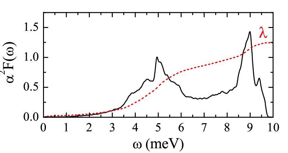
Figure 1 shows the calculated Eliashberg spectral function and the corresponding electron-phonon coupling parameter . We find an overall good agreement with experimental results, [59] although we observe a small (0.5 meV) but non-negligible blueshift of the two peaks in the Eliashberg function. This blueshift is well understood now and arises from the overestimation of the phonon frequencies in the absence of spin-orbit coupling in our calculation. [64, 65] Our calculated electron-phonon coupling =1.24 lies in between the values reported in previous theoretical studies, [63, 62, 39] although it is somewhat smaller than the value 1.55 obtained from tunneling measurements [59] owing to the neglect of spin-orbit coupling.
Figure 2 shows the solutions of the isotropic Eliashberg equations Eqs. (35),(36) for and =0.3 K. Along the imaginary axis the superconducting gap function is purely real and displays a frequency dependence similar to standard plasmon-pole models [Fig. 2(a)]. The continuation of the calculated superconducting gap to the real energy axis is shown in Fig. 2(b). We see that the approximate analytic continuation using Padé functions and the exact iterative analytic continuation yield very similar results. As expected the approximate Padé continuation misses some of the fine features which are instead observed in the exact iterative continuation. Our calculated superconducting gap is in very good agreement with solutions of the Eliashberg equations obtained directly on the real energy axis. [62] In Fig. 2(b) we see that a two-peak structure emerges both in the real part and the imaginary part of . These two peaks occur on the scale of the phonon energies and correlate with those observed in the Eliashberg spectral function of Fig. 1. [5] A detailed analysis shows that the peaks in the real part of the gap function are blueshifted by approximately with respect to the corresponding peaks in .
Figure 3(a) shows the normalized quasiparticle density of unoccupied states obtained from Eq. (40) using the gap function of Fig. 2. As expected the strong van Hove singularity marks the leading edge of the superconducting gap. The fine structure of the density of states around the van Hove singularity [Fig. 3(b)] is the direct signature of the electron-phonon physics and is precisely the basis for direct measurements of the Eliashberg function using tunneling spectroscopy.

Figure 4 shows the superconducting gap function at the Fermi level as a function of temperature, calculated for . The leading edge of the gap at =0 K is found to be =1.24 meV, in good agreement with tunneling measurements yielding 1.33 meV. [59] The superconducting is identified as the temperature at which the gap vanishes. From Fig. 4(a) we find =6.8 K, in very good agreement with previous theoretical studies, [7, 62] and only slightly lower than the experimental datum of 7.2 K. For completeness in Fig. 4(b) and (c) we also explore the sensitivity of the calculated gap and critical temperature to the choice of the Coulomb parameter . As expected, a reduction of the effective Coulomb interaction results in an increase of both and .

IV.3 Magnesium diboride
Within the class of phonon-mediated superconductors MgB2 holds the record of the highest critical temperature, with =39 K.[66] After a decade of intense experimental and theoretical investigations since its discovery, it is now understood that MgB2 is an anisotropic two-gap electron-phonon superconductor. [67, 68, 69, 17, 15] The anisotropy of the superconducting gap is a consequence of the multi-sheet Fermi surface of MgB2, consisting of two hole-like coaxial cylinders arising from the bonding bands, and two hole-like tubular networks arising from the bonding and antibonding bands (see for example Fig. 3 of Ref. 67).
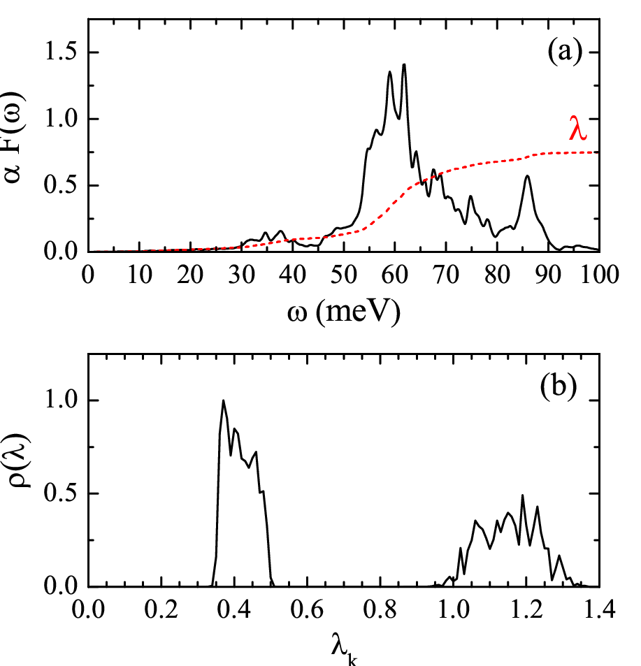
Figure 5(a) shows our calculated isotropic Eliashberg spectral function and electron-phonon coupling strength for MgB2. displays a large dominant peak centered around 60 meV and a second weaker peak centered around 86 meV. The corresponding isotropic electron-phonon coupling strength is =0.748. In order to quantify the different contributions to the coupling strength associated with the sheets and from the sheets of the Fermi surface we evaluate a band- and wavevector- dependent electron-phonon coupling strength defined by . Figure 5(b) shows that the calculated cluster into two separate ranges. The lower range =0.35-0.50 corresponds to the coupling of the Fermi surface sheets, and the higher range 0.95-1.35 corresponds to the coupling of the sheets. The wider range of in the sheets reflects a more pronounced anisotropy with respect to the sheets. The structure of and the calculated coupling strength are in good agreement with previous calculations. [70, 17, 15, 71, 72] In particular our results are in very good agreement with those reported in Ref. 71 where a related interpolation scheme was used. For completeness we show in Table 1 the sensitivity of the calculated average coupling strength on the underlying Brillouin-zone grids, and we compare with previous first-principles calculations.
| Reference | -mesh | -mesh | ||||
|---|---|---|---|---|---|---|
| Bohnen et al. (Ref. 70) | 0.73 | |||||
| Choi et al. (Ref. 17) | 0.73 | |||||
| Floris et al. (Ref. 15) | 0.71 | |||||
| Eiguren et al. (Ref. 71) | 0.776 | |||||
| Calandra et al. (Ref. 72) | 0.741 | |||||
| This work | 0.735 | |||||
| 0.739 | ||||||
| 0.748 | ||||||
| 0.782 | ||||||
| 0.744 | ||||||
| 64000 | 8000 | 0.757 | ||||
| 216000 | 27000 | 0.726 |
Figure 6(a) shows the anisotropic superconducting gap function of MgB2 at =10 K calculated along the imaginary axis using the anisotropic Eliashberg equations Eqs. (21),(22) and =0.16. Figure 6(b) shows the real part of the superconducting gap function along the real energy axis, as obtained from the imaginary axis solutions of Fig 6(a) via the approximate analytic continuation using Padé functions. The two-gap nature of MgB2 emerges in a completely natural way from our implementation. Indeed for each energy two distinct sets of superconducting gaps can be identified and associated with the and the sheets of the Fermi surface. The two gaps are both anisotropic, and the corresponding Fermi-surface averages are meV and meV, respectively. For comparison the experimental values for the gaps lie in the range 2.3-2.8 meV for -band, and 7.0-7.1 meV for -band. [73, 74, 75] As in the case of Pb, the structure that can be observed both in the and superconducting gaps reflect the peaks occuring in the Eliashberg spectral function of Fig. 5.

Figure 7(a) shows the calculated leading edges of the superconducting gaps as a function of temperature. Both the and gaps vanish at the critical temperature =50 K. The corresponding quasiparticle density of states, presented in Fig. 7(b), clearly shows the two-gaps structure of MgB2, in agreement with experiment. [69]
Our calculated critical temperature is larger than the experimentally measured of 39 K, [66] however it is in very good agreement with previous first-principles calculations based on the ME formalism [17] or the SCDFT formalism. [15] At this time it is still unclear whether the overestimation of the experimental critical temperature is due to possible anharmonic effects [17] or to the use of an isotropic Coulomb parameter. [15] In fact, using the anisotropic Eliashberg formalism and a Coulomb parameter , the authors of Ref. 17 find that the calculated decreases from 55 K to 39 K if phonon anharmonicity is taken into account. On the other hand, using the SCDFT formalism the authors of Ref. 15 calculate a critical temperature =22 K when using the complete wavevector-dependent superconducting gap. When employing a band-averaged superconducting gap and various levels of approximations for the Coulomb interaction, the same authors find critical temperatures in the range 30-50 K. [15] A similar sensitivity of the calculated to fine details of the calculations are reported in other studies based on a two-bands approximation to the ME formalism. [14, 38] The origin of the discrepancy between first-principles calculations of the critical temperature of MgB2 and experiment clearly deserves further investigation, however this is beyond the scope of the present manuscript.

The use of electron-phonon Wannier interpolation allows us to investigate the sensitivity of the superconducting gap to the electron and phonon meshes used for the calculations. Figure 8 shows the energy distribution of the -gap at =30 K for eight sets of electron and phonon meshes. If we compare the gaps shown in Fig. 8 and the average coupling strengths reported in Table 1 we see that obtaining converged results for is considerably more challenging than for . For example, when using the same -points mesh () and different -points meshes ( and ), the spread of the superconducting gap distribution changes from 2.5 meV to 1.5 meV, while the average coupling strength is essentially unaffected. The same observation applies when we compare results for the same -points mesh ( but different -points meshes ( and ). These differences highlight the difficulty of describing anisotropic quantities, and point out the need of having a very dense sampling of the Brillouin zone not only for the electrons but also for the phonons. For this reason the combination of the Eliashberg formalism with electron-phonon Wannier interpolation demonstrated in this work provides an ideal computational tool for investigating anisotropic superconductors.

V CONCLUSIONS
In summary we developed a computational method which combines the anisotropic Migdal-Eliashberg formalism with electron-phonon interpolation based on maximally-localized Wannier functions (EPW). Our new method allows us to calculate the momentum- and band-resolved superconducting gap both effectively and accurately using a very fine description of electron-phonon scattering processes on the Fermi surface. In order to demonstrate our methodology we reported a comprehensive set of tests on two representative superconductors, namely Pb and MgB2, and validated our approach against previous first-principles calculations as well as experiment. We discussed the performance of two analytic continuation methods for obtaining the superconducting gap on the real energy axis, and we investigated the sensitivity of the calculated gaps on the underlying choice of the Brillouin-zone grids for electrons and phonons.
In order to set a road map for first-principles studies of superconductors we now discuss the key approximations involved in the present approach and suggest possible avenues for future developments. The main approximations leading to Eqs. (21),(22) are as follows: (i) vertex corrections in the diagrammatic expansion of the electron self-energy are neglected following Migdal’s theorem, (ii) the self-energy is assumed to be diagonal in band indices, (iii) the Eliashberg equations are restricted to bands near the Fermi level, (iv) the density of states near the Fermi level is assumed to be constant, and (v) the Coulomb interaction is described by an empirical parameter. [2, 35, 36]
Regarding approximation (i), it is well known that Migdal’s theorem can break down for large electron-phonon coupling or in the presence of Fermi-surface nesting. [2, 35] In this area the availability of electron-phonon matrix elements at a very small computational cost, as provided by our method, could be used as a starting point to explore the effects of vertex corrections beyond Migdal’s approximation. For example the evaluation of the first non-crossing diagram should not constitute a major challenge, at least in the normal state. This may help assessing the numerical error introduced by Migdal’s approximation.
Going beyond approximation (ii) is computationally challenging since the Green’s function and the self-energy should be treated as matrices in the band indices. [76, 77] This step would increase substantially the complexity of the formalism since the inversion of the Dyson’s equation would require matrix operations. Given the small energies associated with the superconducting gap it is reasonable to expect that off-diagonal terms should not play an important role in simple cases. However in the presence of degeneracies, and in particular in Jahn-Teller systems, the correct description of these terms may prove critical. [78]
It should be possible, at least in principle, to remove approximation (iii) by including bands away from the Fermi level in the calculations. Here the difficulty is purely on the computational side, and for simple systems this should be doable. However relaxing this constraint would also introduce one additional equation [Eq. (16)] in order to calculate the correct quasiparticle shifts and impose the conservation of charge in the system.
The assumption (iv) of a constant density of states near the Fermi level obviously breaks down for materials exhibiting structure in the density of states on the scale of the phonon energy. In theses cases it has been shown that the energy dependence of density of states can be retained within the isotropic approximation to the Eliashberg equations. [2, 79, 35] We are planning to include this possibility in our methodology in the future.
Lastly, approximation (v) means that in the present implementation the Coulomb repulsion between electrons remains described at the empirical level as an adjustable parameter. In order to remove this limitation our first step will be to evaluate the Coulomb parameter using the dielectric matrix in the random-phase approximation. [80] In the longer term it would be desirable to introduce inside Eq. (22) matrix elements of the screened Coulomb interaction calculated using the Sternheimer-GW method of Ref. 81.
We hope that the method reported here will prove useful to the superconductivity community as a robust and rigorous procedure for shedding light on existing superconductors and possibly for predicting new superconductors yet to be discovered.
Acknowledgements.
E.R.M. was funded by Marie Curie IEF project FP7-PEOPLE-2009-IEF-252586. F.G. acknowledges support from the European Research Council under the EU FP7/ERC grant no. 239578.References
- [1] J. P. Carbotte, Rev. Mod. Physics 62, 1027 (1990).
- [2] P. B. Allen, and B. Mitrović, Solid State Phys. 37, 1 (1982).
- [3] F. Marsiglio, and J. P. Carbotte, in Superconductivity, edited by K. H. Bennemann, and J. B. Ketterson (Springer 2008), Vol. 1, page 73.
- [4] D. J. Scalapino, J. R. Schrieffer, and J. W. Wilkins, Phys. Rev. 148, 263 (1966).
- [5] D. J. Scalapino in Superconductivity, edited by R. D. Parks (Dekker, New York, 1969), Vol. 1, page 449.
- [6] M. Lüders, M. A. L. Marques, N. N. Lathiotakis, A. Floris, G. Profeta, L. Fast, A. Continenza, S. Massidda, and E. K. U. Gross, Phys. Rev. B 72, 024545 (2005).
- [7] M. A. L. Marques, M. Lüders, N. N. Lathiotakis, G. Profeta, A. Floris, L. Fast, A. Continenza, E. K. U. Gross, and S. Massidda, Phys. Rev. B 72, 024546 (2005).
- [8] J. Bardeen, L. N. Cooper, and J. R. Schrieffer, Phys. Rev. 108, 1175 (1957).
- [9] W. L. McMillan, Phys. Rev. 167, 331 (1968).
- [10] A. B. Migdal, Zh. Eksperim. i Teor. Fiz. 34, 1438 (1958) [Sov. Phys. JETP 7, 996 (1958)].
- [11] G. M. Eliashberg, Zh. Eksperim. i Teor. Fiz. 38, 966 (1960) [Sov. Phys. JETP 11, 696 (1960)].
- [12] A. A. Golubov, J. Kortus, O. V. Dolgov, O. Jepsen, Y. Kong, O. K. Andersen, B. J. Gibson, K. Ahn, and R. K. Kremer, J. Phys.: Condens. Matter 14, 1353 (2002).
- [13] H. J. Choi, M. L. Cohen, and S. G. Louie, Phys. Rev. B 73, 104520 (2006).
- [14] I. I. Mazin, O. K. Andersen, O. Jepsen, A. A. Golubov, O. V. Dolgov, and J. Kortus, Phys. Rev. B 69, 056501 (2004).
- [15] A. Floris, G. Profeta, N. N. Lathiotakis, M. Lüders, M. A. L. Marques, C. Franchini, E. K. U. Gross, A. Continenza, and S. Massidda, Phys. Rev. Lett. 94, 037004 (2005).
- [16] A. Sanna, S. Pittalis, J. K. Dewhurst, M. Monni, S. Sharma, G. Ummarino, S. Massidda, and E. K. U. Gross, Phys. Rev. B 85, 184514 (2012).
- [17] H. J. Choi, D. Roundy, H. Sun, M. L. Cohen, and S. G. Louie, Nature (London) 418, 758 (202); H. J. Choi, D. Roundy, H. Sun, M. L. Cohen, and S. G. Louie, Phys. Rev. B 66 , 020513(R) (2002).
- [18] A. Sanna, G. Profeta, A. Floris, A. Marini, E. K. U. Gross, and S. Massidda, Phys. Rev. B 75, 020511(R) (2007).
- [19] G. Savini, A. C. Ferrari, and F. Giustino, Phys. Rev. Lett. 105, 037002 (2010).
- [20] A. N. Kolmogorov and S. Curtarolo, Phys. Rev. B 73, 180501(R) (2006).
- [21] A. N. Kolmogorov, M. Calandra, and S. Curtarolo, Phys. Rev. B 78, 094520 (2008).
- [22] A. N. Kolmogorov, S. Shah, E. R. Margine, A. F. Bialon, T. Hammerschmidt, and R. Drautz, Phys. Rev. Lett. 105, 217003 (2010).
- [23] A. Jain, G. Hautier, C. J. Moore, S. P. Ong, C. C. Fischer, T. Mueller, K. A. Persson, and G. Ceder, Computational Materials Science 50, 2295 (2011).
- [24] K. Yang, W. Setyawan, S. Wang, M. Buongiorno-Nardelli, and S. Curtarolo, Nature Materials 11, 614 (2012).
- [25] A. Damascelli, Z. Hussain, Z.-X. Shen, Rev. Mod. Phys. 75, 473 (2003)
- [26] O. Fischer, M. Kugler, I. Maggio-Aprile, C. Berthod, and C. Renner, Rev. Mod. Phys. 79, 353 (2007).
- [27] F. Giustino, M. L. Cohen, and S. G. Louie, Phys. Rev. B 76, 165108 (2007).
- [28] N. Marzari, A. A. Mostofi, J. R. Yates, I. Souza, and D. Vanderbilt, Rev. Mod. Phys. 84, 1419 (2012).
- [29] J. R. Yates, X. Wang, D. Vanderbilt, and I. Souza, Phys. Rev. B 75, 195121 (2007).
- [30] X. Wang, J. R. Yates, I. Souza, and D. Vanderbilt, Phys. Rev. B 74, 195118 (2006).
- [31] D. R. Hamann and D. Vanderbilt, Phys. Rev. B 79, 045109 (2009).
- [32] J. Noffsinger, F. Giustino, B. D. Malonea, C.-H. Park, S. G. Louie, and M. L. Cohen, Comput. Phys. Commun. 181, 2140 (2010).
- [33] Y. Nambu, Phys. Rev. 117, 648 (1960).
- [34] L. P. Gorkov, Sov. Phys. JETP 7, 505 (1958).
- [35] W. E. Pickett, Phys. Rev. B 26, 1186 (1982).
- [36] P. B. Allen, Phys. Rev. B 13, 1416 (1976).
- [37] P. Morel, and P. W. Anderson, Phys. Rev. B 125, 1263 (1962).
- [38] C.-Y. Moon, Y.-H. Kim, and K. J. Chang, Phys. Rev. B 70, 104522 (2004).
- [39] A. Y. Liu and A. A. Quong, Phys. Rev B 53, R7575 (1996).
- [40] J. Bauer, J. E. Han, and O. Gunnarsson, arXiv:1202.5051v2.
- [41] M. J. Holcomb, Phys. Rev. B 54, 6648 (1996).
- [42] H. J. Vidberg, and J. W. Serene, J. Low Temp. Phys. 29, 179 (1977).
- [43] C. R. Leavens, and D. S. Ritchie, Solid State Commun. 53, 137 (1985).
- [44] F. Marsiglio, M. Schossmann, and J. P. Carbotte, Phys. Rev. B 37, 4965 (1988).
- [45] K. S. D. Beach, R. J. Gooding, and F. Marsiglio, Phys. Rev. B 61, 5147 (2000).
- [46] S. Baroni, S. de Gironcoli, A. Dal Corso, and P. Giannozzi, Rev. Mod. Phys. 73, 515 (2001).
- [47] N. Marzari and D. Vanderbilt, Phys. Rev. B 56, 12847 (1997).
- [48] I. Souza, N. Marzari, and D. Vanderbilt, Phys. Rev. B 65, 035109 (2001).
- [49] P. Giannozzi et al., J. Phys. Condens. Matter 21, 395502 (2009).
- [50] A. A. Mostofi, J. R. Yates, Y.-S. Lee, I. Souza, D. Vanderbilt, and N. Marzari, Comput. Phys. Comm. 178, 685 (2008).
- [51] P. B. Allen and R. C. Dynes, Phys. Rev. B 12, 905 (1975).
- [52] C. G. Broyden, Math. Comput. 19, 577 (1965).
- [53] D. D. Johnson, Phys. Rev. B 38, 12807 (1988).
- [54] D. M. Ceperley and B. J. Alder, Phys. Rev. Lett. 45, 566 (1980).
- [55] J. P. Perdew and A. Zunger, Phys. Rev. B 23, 5048 (1981).
- [56] N. Troullier and J. L. Martins, Phys. Rev. B 43, 1993 (1991).
- [57] M. Fuchs and M. Scheffler, Comput. Phys. Commun. 119, 67 (1999).
- [58] M. Methfessel and A. T. Paxton, Phys. Rev. B 40, 3616 (1989).
- [59] W. L. McMillan and J. M. Rowell, in Superconductivity, edited by R. D. Parks (Dekker, New York, 1969), Vol 1, page 601.
- [60] B. L. Blackford and R. H. March, Phys. Rev. 186, 397 (1969).
- [61] G. I. Lykken, A. L. Geiger, K. S. Dy, and E. N. Mitchell, Phys. Rev. B 4, 1523 (1971).
- [62] P. G. Tomlinson and J. P. Carbotte, Phys. Rev B 13, 4738 (1976).
- [63] A. Floris, A. Sanna, S. Massidda, and E. K. U. Gross, Phys. Rev B 75, 054508 (2007).
- [64] A. Dal Corso, J. Phys.: Condens. Matter 20, 445202 (2008).
- [65] R. Heid, K.-P. Bohnen, I. Yu. Sklyadneva, and E. V. Chulkov, Phys. Rev B 81, 174527 (2010).
- [66] J. Nagamatsu, N. Nakagawa, T. Muranaka, Y. Zenitani, and J. Akimitsu, Nature (London) 410, 63 (2001).
- [67] J. Kortus, I. I. Mazin, K. D. Belashchenko, V. P. Antropov, and L. L. Boyer, Phys. Rev. Lett. 86, 4656 (2001).
- [68] A. Y. Liu, I. I. Mazin, and J. Kortus, Phys. Rev. Lett. 87, 087005 (2001).
- [69] F. Giubileo, D. Roditchev, W. Sacks, R. Lamy, D. X. Thanh, J. Klein, S. Miraglia, D. Fruchart, J. Marcus, and Ph. Monod, Phys. Rev. Lett. 87, 177008 (2001).
- [70] K.-P. Bohnen, R. Heid, and B. Renker, Phys. Rev. Lett. 86, 5771 (2001).
- [71] A. Eiguren and C. Ambrosch-Draxl, Phys. Rev. B 78, 045124 (2008).
- [72] M. Calandra, G. Profeta, and F. Mauri, Phys. Rev. B 82, 165111 (2010).
- [73] M. Iavarone, G. Karapetrov, A. E. Koshelev, W. K. Kwok, G. W. Crabtree, D. G. Hinks, W. N. Kang, E.-M. Choi, H. J. Kim, H.-J. Kim, and S. I. Lee, Phys. Rev. Lett. 89, 187002 (2002).
- [74] P. Szabó, P. Samuely, J. Kačmarčík, T. Klein, J. Marcus, D. Fruchart, S. Miraglia, C. Marcenat, and A. G. M. Jansen, Phys. Rev. Lett. 87, 137005 (2001).
- [75] R. S. Gonnelli, D. Daghero, G. A. Ummarino, V. A. Stepanov, J. Jun, S. M. Kazakov, and J. Karpinski, Phys. Rev. Lett. 89, 247004 (2002).
- [76] J. C. Garland, Phys. Rev. 153, 460 (1967).
- [77] P. B. Allen, Phys. Rev. B 18, 5217 (1978).
- [78] O. Gunnarsson, Rev. Mod. Phys. 69, 575 (1997).
- [79] W. E. Pickett, Phys. Rev. B 21, 3897 (1980).
- [80] K.-H. Lee, K. J. Chang, and M. L. Cohen, Phys. Rev. B 52, 1425 (1995).
- [81] F. Giustino, M. L. Cohen, and S. G. Louie, Phys. Rev. B 81, 115105 (2010).